2.1. Sound prediction using Lighthill's acoustic analogy

The fluctuating sound pressure, $p$, in the acoustic field can be computed using Lighthill's acoustic analogy (Lighthill Reference Lighthill1952)

(2.1)\begin{equation} \frac{1}{c^2_\infty }\frac{\partial^2 p}{\partial t^2} - \nabla^2 p = \frac{\partial^2 \boldsymbol{\mathsf{T}}_{ij}}{\partial x_i \partial x_j}, \end{equation}

where $t$ is time, $c_\infty$ is the ambient speed of sound, $x$ are the source coordinates and $\boldsymbol{\mathsf{T}}_{ij}$ is the Lighthill stress tensor

(2.2)\begin{equation} \boldsymbol{\mathsf{T}}_{ij} = \rho u_i u_j -\tau_{ij}+(p-c^2_{\infty}\rho)\delta_{ij}, \end{equation}

where $u$ is fluid velocity, $\tau$ are viscous stresses and $\rho$ is density. In high-Reynolds-number flows, viscous contributions are minimal (Freund Reference Freund2001) and can hence be neglected. The term $(p-c^2_{\infty }\rho )\delta _{ij}$ represents noise generation due to entropic inhomogeneity. Bodony & Lele (Reference Bodony and Lele2008) have shown that there is significant cancellation between the entropic term and the momentum component ($\rho u_i u_j$) at downstream observer angles in an ideally expanded supersonic jet. This cancellation, however, is negligible at sideline directions where we expect BBSAN to dominate. This view is also echoed by Freund (Reference Freund2003) who found that sideline ($\theta =90^{\circ }$) noise is dominated by Lighthill source terms that are largely independent of the entropic term. For BBSAN specifically, evidence also exists which suggests the contribution of the entropic term is negligible compared with the momentum terms in unheated shock-containing jets (Ray & Lele Reference Ray and Lele2007; Morris & Miller Reference Morris and Miller2010). From these observations, we choose to neglect the entropic term as a first approximation, as it greatly simplifies the model. The stress tensor is hence approximated by

(2.3)\begin{equation} \boldsymbol{\mathsf{T}}_{ij} \approx \rho u_i u_j . \end{equation}

A solution to (2.1) for the acoustic pressure field in the frequency domain, $\omega$, is given by

(2.4)\begin{equation} p(\boldsymbol{y};\omega) = \int_V \frac{\partial^2 \hat{\boldsymbol{\mathsf{T}}}_{ij}(\boldsymbol{x};\omega)}{\partial x_i \partial x_j} G_{0}(\boldsymbol{x},\boldsymbol{y};\omega)\,\textrm{d}\boldsymbol{x} , \end{equation}

where $\hat {\boldsymbol{\mathsf{T}}}_{ij}$ is the time Fourier-transformed quantity of $\boldsymbol{\mathsf{T}}_{ij}$. An implicit $\exp (-\textrm {i} \omega t)$ dependence on $t$ is assumed. The observer $\boldsymbol {y}$ and the source $\boldsymbol {x}$ positions are in spherical and cylindrical coordinates, respectively, as shown in figure 1. The prescribed cylindrical coordinate system $(x,r,\phi )$ has the $x$-axis aligned with the jet centreline, $r$ is the radial separation and $\phi$ the azimuthal angle. For the observer coordinates $(R,\theta ,\phi )$, the same azimuthal coordinate of the cylindrical system is used, the polar angle $\theta$ is defined from the downstream jet axis and $R$ is the distance from the origin. The integration is carried out in the volume $V$ where the source is non-zero. We define $G_0$ as the free-field Green's function

(2.5)\begin{equation} G_{0}(\boldsymbol{x},\boldsymbol{y},\omega) = \frac{1}{4 {\rm \pi}} \frac{\exp({\mathrm{i}k_a | \boldsymbol{x}-\boldsymbol{y} |})}{|\boldsymbol{x}-\boldsymbol{y}|} , \end{equation}

where $k_a=\omega /c_\infty$ is the acoustic wavenumber. We also transfer the second derivative of $\boldsymbol{\mathsf{T}}_{ij}$ onto the Green's function by applying the divergence theorem and assuming the resulting surface integral to be negligible (Goldstein Reference Goldstein1976). This makes evaluation of the integral less sensitive to spurious fluctuations in the stress tensor due to numerical noise. Acoustic sources embedded in high-speed flows may also be subjected to propagation effects such as refraction (Tam & Auriault Reference Tam and Auriault1998). For predicting far-field BBSAN from an unheated single-stream shock-containing jet, at polar angles $50^{\circ } \leq \theta \leq 130^{\circ }$, Miller & Morris (Reference Miller and Morris2012) show that a free-field Green's function provides adequate results when compared with predictions which included propagation effects.

Figure 1. Schematic of experimental set-up with the prescribed source $(x,r,\phi )$ and observer $(R,\theta ,\phi )$ coordinate systems.

Equation (2.4) is appropriate for time-periodic $\hat {\boldsymbol{\mathsf{T}}}_{ij}$, or for a $\boldsymbol{\mathsf{T}}_{ij}$ that may be Fourier transformed in time. Since flow fluctuations are not square-integrable functions, as required for the application of a Fourier transform, one cannot obtain the sound field through direct application of (2.4), as the computation of a Fourier transform in this case would require windowing in time. One way to circumvent this issue (Landahl, Mollo-Christensen & Korman Reference Landahl, Mollo-Christensen and Korman1989; Cavalieri & Agarwal Reference Cavalieri and Agarwal2014; Baqui et al. Reference Baqui, Agarwal, Cavalieri and Sinayoko2015) is to compute the power spectral density (PSD) of the acoustic field. For a given frequency $\omega$, the PSD $\langle p(\boldsymbol {y},\omega )p^*(\boldsymbol {y},\omega ) \rangle$ is given by

(2.6)\begin{align} \langle p(\boldsymbol{y};\omega)p^*(\boldsymbol{y};\omega) \rangle = \int_V \int_V \langle \boldsymbol{\mathsf{T}}_{ij}(\boldsymbol{x_1};\omega)\boldsymbol{\mathsf{T}}^*_{ij}(\boldsymbol{x_2};\omega)\rangle \frac{\partial^2 G_{0}(\boldsymbol{x_1},\boldsymbol{y};\omega)}{\partial x_i \partial x_j} \frac{\partial^2 G^*_{0}(\boldsymbol{x_2},\boldsymbol{y};\omega)}{\partial x_i \partial x_j}\, \textrm{d}\boldsymbol{x_1}\, \textrm{d}\boldsymbol{x_2} , \end{align}

where $\langle \; \rangle$ denotes an expected value, the quantity $\langle \boldsymbol{\mathsf{T}}_{ij}(\boldsymbol {x_1},\omega )\boldsymbol{\mathsf{T}}^*_{ij}(\boldsymbol {x_2},\omega )\rangle$ is the cross-spectral density (CSD) of the stress tensor for a pair of points $\boldsymbol {x_1}$ and $\boldsymbol {x_2}$, $^*$ denotes the complex conjugate and we have dropped the ‘hats’ for convenience. We exploit axisymmetry by expanding $\boldsymbol{\mathsf{T}}_{ij}$ as a series of azimuthal modes (Michalke & Fuchs Reference Michalke and Fuchs1975); noting that there is a direct correspondence between the azimuthal mode of the source and that of the sound field (Michalke Reference Michalke1970; Cavalieri et al. Reference Cavalieri, Jordan, Colonius and Gervais2012). By taking a Fourier transform of the source in azimuth, we can compute azimuthal mode $m$ of the far-field pressure to be

(2.7)\begin{align} \langle p(R,\theta;m,\omega)p^*(R,\theta;m,\omega) \rangle = \int_V \int_V \langle \boldsymbol{\mathsf{S}}_{ij}(m,\omega)\rangle \frac{\partial^2 G_{0,1}(m,\omega)}{\partial x_i \partial x_j} \frac{\partial^2 G^*_{0,2}(m,\omega)}{\partial x_i \partial x_j} \,\textrm{d}\boldsymbol{x_1}\,\textrm{d}\boldsymbol{x_2} , \end{align}

where we have dropped the spatial coordinates of the source for compactness, $G_{0,1}$ and $G_{0,2}$ represent the Green's functions at source location $\boldsymbol {x_1}$ and $\boldsymbol {x_2}$, respectively, and $\boldsymbol{\mathsf{S}}_{ij}$ represents the CSD of the stress tensor

(2.8)\begin{equation} \boldsymbol{\mathsf{S}}_{ij}(x_1,r_1,x_2,r_2;m,\omega) = \boldsymbol{\mathsf{T}}_{ij}(x_1,r_1;m,\omega)\boldsymbol{\mathsf{T}}^*_{ij}(x_2,r_2;m,\omega) . \end{equation}

2.2. Equivalent BBSAN source model

The proposed BBSAN model is based on the idea that the source only involves fluctuations associated with interactions between the turbulent component ($\boldsymbol {q}_t$) and shock perturbations ($\boldsymbol {q}_s$). This assumption has been made by a number of authors (Tam & Tanna Reference Tam and Tanna1982; Lele Reference Lele2005; Ray & Lele Reference Ray and Lele2007; Wong et al. Reference Wong, Jordan, Honnery and Edgington-Mitchell2019b), where different descriptions of $\boldsymbol {q}_t$ and $\boldsymbol {q}_s$ were investigated. We follow this approach and, similar to Wong et al. (Reference Wong, Jordan, Honnery and Edgington-Mitchell2019b), adopt a two-point description of the source.

As performed by Tam (Reference Tam1987), we decompose the flow variables according to

(2.9)\begin{equation} \boldsymbol{q} = \boldsymbol{\bar{q}} + \boldsymbol{q}_t + \boldsymbol{q}_s , \end{equation}

where $\boldsymbol {\bar {q}}$, $\boldsymbol {q}_t$, $\boldsymbol {q}_s$ are the mean, turbulent and shock-cell disturbance components, respectively. We take the mean component to be the time-averaged flow of an ideally expanded jet. The vector $\boldsymbol {q}$ refers to the dependent flow variables of interest, $\boldsymbol {q} = [u_x, u_r, u_\phi , T, \rho ]^{T}$, where $u_x$, $u_r$ and $u_\phi$ are the axial, radial and azimuthal velocity components, respectively. The thermodynamic variables include $T$ and $\rho$ which are the temperature and the density of the fluid, respectively. The decomposition in (2.9) is substituted into the stress tensor in (2.3),

(2.10)\begin{equation} \boldsymbol{\mathsf{T}}_{ij} \approx (\bar{\rho}+\rho_s+\rho_t)( \bar{u}_i+u_{i,t}+u_{i,s})( \bar{u}_j+u_{j,t}+u_{j,s}) . \end{equation}

Assuming that BBSAN is generated by turbulence-shock interaction, the expression for $\boldsymbol{\mathsf{T}}_{ij}$, as shown in Appendix A, can be simplified to

(2.11)\begin{equation} \boldsymbol{\mathsf{T}}_{ij} \approx \bar{\rho}(u_{i,t}u_{j,s}+u_{i,s}u_{j,t})+\rho_s(\bar{u}_iu_{j,t}+\bar{u}_ju_{i,t})+\rho_t(\bar{u}_iu_{j,s}+\bar{u}_ju_{i,s}) . \end{equation}

Here we highlight some characteristics of (2.11). Firstly, this representation of $\boldsymbol{\mathsf{T}}_{ij}$ does not account for turbulent mixing noise since only turbulence-shock interaction terms are retained (Appendix A). This is justified by the minimal contribution of mixing noise at the frequencies and polar positions where BBSAN is dominant (Viswanathan Reference Viswanathan2006; Viswanathan et al. Reference Viswanathan, Alkislar and Czech2010). Agreement with measured acoustic data at low frequencies and downstream polar angles would therefore not be expected. Secondly, unlike previous wavepacket models in subsonic jets (Cavalieri et al. Reference Cavalieri, Jordan, Agarwal and Gervais2011; Piantanida et al. Reference Piantanida, Jaunet, Huber, Wolf, Jordan and Cavalieri2016; Maia et al. Reference Maia, Jordan, Cavalieri and Jaunet2019), we retain all velocity components of $\boldsymbol{\mathsf{T}}_{ij}$ in order to improve predictions in the sideline direction. We also note that while (2.11) is similar to the source term derived by Lele (Reference Lele2005), we retain the double-divergence and have discarded the entropic term.

The BBSAN sound field can be obtained using (2.7) and (2.11). Unlike previous two-point wavepacket modelling work (Maia et al. Reference Maia, Jordan, Cavalieri and Jaunet2019; Wong et al. Reference Wong, Jordan, Honnery and Edgington-Mitchell2019b), we choose to relax the line-source simplification and work with a full volumetric source instead. The $\boldsymbol {q}_t$ and $\boldsymbol {q}_s$ parts of $\boldsymbol{\mathsf{T}}_{ij}$ are each computed using numerical and experimental databases, respectively, as shown in § 4, before being combined according to (2.11). The source domain extends from $0 \leq x \leq 25D$ and $0 \leq r \leq 2D$ in the axial and radial directions, respectively. An appropriate window function, summarised further in § 5.1, is used to ensure no artificial overprediction of the acoustic field (Obrist & Kleiser Reference Obrist and Kleiser2007; Martínez-Lera & Schram Reference Martínez-Lera and Schram2008).

3.1. Numerical database: LES of $M_j=1.5$ ideally expanded jet

The turbulent flow quantities $\boldsymbol {q}_t$ are extracted from an LES of an isothermal ideally expanded $M_j=1.5$ supersonic jet. An extension to the previous LES by Brès et al. (Reference Brès, Ham, Nichols and Lele2017), this simulation was performed using the compressible flow solver ‘Charles’, developed at Cascade Technologies, on an unstructured adapted grid with 40 million cells. The jet issues from a round converging–diverging nozzle. The Reynolds number based on nozzle exit conditions is $Re = \rho _j U_j D / \mu _j = 1.76 \times 10^6$, matching the experiment carried out at the United Technologies Research Center (UTRC) anechoic jet facility (Schlinker et al. Reference Schlinker, Simonich, Shannon, Reba, Colonius, Gudmundsson and Ladeinde2009). Near-wall adaptive mesh refinement is employed on the internal nozzle surface to closely model the boundary layer inside the nozzle, leading to turbulent boundary layer profiles at the exit (Brès et al. Reference Brès, Jordan, Jaunet, Le Rallic, Cavalieri, Towne, Lele, Colonius and Schmidt2018). A slow coflow of $M_{co} = 0.1$ is also included in the simulation to match the UTRC experimental conditions. As the LES jet is shock-free, direct computation of the BBSAN sound field via an FW–H surface is not possible.

To facilitate postprocessing and analysis, the LES data is interpolated from the original unstructured LES grid onto a structured cylindrical grid with uniform spacing in azimuth. The three-dimensional cylindrical grid is defined over $0 \leq x/D \leq 30$, $0 \leq r/D \leq 6$, with $(n_x, n_r, n_{\theta } ) = (698, 136, 128)$, where $n_x$, $n_r$ and $n_{\theta }$ are the number of grid points in the streamwise, radial and azimuthal direction, respectively. The simulation time step, in acoustic time units, is $\Delta t c_\infty /D = 0.0004$ and the database is sampled every $\Delta t c_\infty /D = 0.1$. Snapshots are therefore recorded every 250 time steps, corresponding to a cutoff (Nyquist) frequency of $St = \Delta f D / U_j = 3.33$. The simulation parameters are summarised in table 2. Further details on the numerical strategy can be found in Brès et al. (Reference Brès, Ham, Nichols and Lele2017).

Table 2. Summary of LES parameters.

3.2. Experimental database: PIV of $M_j=1.45$ underexpanded jet

For the description of $\boldsymbol {q}_s$, we resort to high spatial resolution two-dimensional, two component PIV measurements of a cold screeching underexpanded supersonic jet with an ideally expanded Mach number of $M_j=1.45$. The data was previously acquired at the supersonic jet facility at the Laboratory for Turbulence Research in Aerospace and Combustion (LTRAC) (Edgington-Mitchell, Honnery & Soria Reference Edgington-Mitchell, Honnery and Soria2014a). The facility has been used extensively in previous experimental studies of shock-containing supersonic jets (Edgington-Mitchell et al. Reference Edgington-Mitchell, Oberleithner, Honnery and Soria2014b; Weightman et al. Reference Weightman, Amili, Honnery, Edgington-Mitchell and Soria2019). The facility is not anechoic and noise measurements were not conducted.

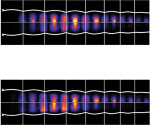
The final field of view of the images is $10D$ and $2.2D$, with $(N_x,N_y)= (1000,75)$, in the axial and radial directions, respectively. The optical resolution of the images is $0.001D/px$. Full details of the experimental set-up and postprocessing techniques are described in Edgington-Mitchell et al. (Reference Edgington-Mitchell, Oberleithner, Honnery and Soria2014b). Mean axial and radial velocity fields from both the LES and PIV data are shown in figure 2.

Figure 2. The LES (a,c,e) and PIV (b,d,f) $x-r$ contour mean fields for ideally expanded and shock-containing jets, respectively; streamwise velocity (a,b), radial velocity (c,d) and density (e,f). Flow quantities are normalised by the ideally expanded condition.

3.3. Acoustic database: far-field acoustic measurements $M_j=1.5$ underexpanded jet

The acoustic measurements were performed at the Supersonic Jet Anechoic Facility (SJAF) at Monash University. This is a different facility to the jet rig used to acquire the PIV measurements in § 3.2. Most importantly, the jet is mounted inside a fully enclosed anechoic chamber. The chamber walls are treated with 400 mm foam wedges, corresponding to a cutoff frequency of 500 Hz. The interior chamber dimensions (wedge-tip-to-wedge-tip) are $1.5\ \textrm {m}\times 1.2\ \textrm {m} \times 1.4\ \textrm {m}$. The jet exits out of a converging-round nozzle with an exit diameter of $D=8\ \textrm {mm}$. Unheated compressed air is supplied to the jet at $NPR=3.67$, corresponding to the same $M_j$ as the LES case.

Acoustic measurements were performed using an azimuthal ring of radius $11D$ and a schematic of the experimental set-up is shown in figure 1. The CSD of pressure, as a function of azimuthal separation, was obtained using a pair of G.R.A.S. Type 46BE 1/4” preamplified microphones with a frequency range of 4 Hz–100 kHz, one fixed and the other moving in the azimuthal direction. Using the postprocessing methodology detailed in Wong et al. (Reference Wong, Kirby, Jordan and Edgington-Mitchell2020), the measured sound fields were azimuthally decomposed. The azimuthal array is traversed axially to acquire measurements at different polar angles over a cylindrical surface. The radial distance $r=11D$ is therefore constant, while observer distance $R$ changes. A detailed description of the experimental set-up can be found in Wong et al. (Reference Wong, Kirby, Jordan and Edgington-Mitchell2020).

The motivation for using azimuthally decomposed data is twofold. Firstly, the measurements of previous authors (Suzuki Reference Suzuki2016; Arroyo & Moreau Reference Arroyo and Moreau2019; Wong et al. Reference Wong, Kirby, Jordan and Edgington-Mitchell2020) suggest the spectrum of each azimuthal mode differs from the total sound field; an increasing number of modes is required to reconstruct the total signal at high frequencies and for upstream angles. Secondly, in a linear acoustic problem such as this, Michalke & Fuchs (Reference Michalke and Fuchs1975) demonstrated that there exists a direct correspondence between the acoustic source $\boldsymbol{\mathsf{S}}_{ij}$ and the far-field sound of the same azimuthal mode.

4.1. Eduction of shock-cell component

Similar to Tam & Tanna (Reference Tam and Tanna1982) and Lele (Reference Lele2005), we adopt the Pack and Prandtl (P–P) (Prandtl Reference Prandtl1904; Pack Reference Pack1950) approximation of the shock-cell structure. The shocks are modelled as small disturbances superimposed over an ideally expanded jet. The model assumes the jet to be bounded by a vortex sheet, allowing the periodic shock-cell structure to be represented by a sum of zero-frequency waves. Good agreement is found close to the nozzle exit, where the shear layer is thin, but worsens downstream as the shear layer thickens, invalidating the vortex sheet assumption (Tam, Jackson & Seiner Reference Tam, Jackson and Seiner1985). With increasing distance from the nozzle exit, the model therefore fails to predict the decay in shock strength and the accompanying contraction in shock-cell spacing. Since the BBSAN source is reported to extend several jet diameters downstream (Seiner & Norum Reference Seiner and Norum1980; Gojon & Bogey Reference Gojon and Bogey2017), any disagreement between the vortex sheet model and measured jet characteristics is likely to lead to incorrect peak frequency predictions.

While the shock-cell disturbances may be extracted from data (e.g. PIV) or computed by solving linear locally parallel stability equations (Tam et al. Reference Tam, Jackson and Seiner1985), the shock perturbations have a smooth and nearly sinusoidal variation towards the end of the potential core. The P–P model therefore remains an attractive simplified approach for capturing the mean shock structure; indeed, source models adopting the approximation are able to reproduce the main features of BBSAN, including higher-order BBSAN peaks (Tam & Tanna Reference Tam and Tanna1982; Wong et al. Reference Wong, Jordan, Honnery and Edgington-Mitchell2019b). To remedy the shortfalls of the vortex sheet assumption, we use the PIV database to modify the P–P solution in order to arrive at a more realistic model.

The jet is modelled as a cylindrical vortex sheet (Lessen, Fox & Zien Reference Lessen, Fox and Zien1965), and the normal mode ansatz is introduced:

(4.1)\begin{equation} \boldsymbol{q}_{s,vortex}(x,r,\theta,t) = \sum_{\omega} \sum_{k_s} \sum_{m_s} \boldsymbol{\hat{q}}_s(r)\exp({\textrm{i}\omega_st - \textrm{i}k_sx - \textrm{i}m_s\phi}) , \end{equation}

where $\omega _s$ is frequency, $k_{s}$ and $m_s$ are axial and azimuthal wavenumbers. By assuming the shock-cell disturbances are stationary ($\omega _s=0$) and axisymmetric ($m_s=0$), we obtain for each dependent variable of interest $\boldsymbol {q}_s$,

(4.2)\begin{equation} q_{s,vortex}(x,r) = \sum^\infty_{n=1}A_n \textrm{J}_0(\alpha_nr)\exp({-\textrm{i}k_{s_n}x}) , \end{equation}

where $A_n$ is the amplitude of each shock-cell mode $n$, $k_{s_n}$ are the axial wavenumbers and $\textrm {J}_0$ is the zeroth-order Bessel function of the first kind. The boundary condition for constant velocity on the jet boundary (Pack Reference Pack1950) requires that the values of $\alpha _n$ satisfy

(4.3)\begin{equation} \textrm{J}_0(\alpha_n) = 0 , \end{equation}

and from the dispersion relation, we obtain the sequence of axial wavenumbers to be

(4.4)\begin{equation} k_{s_n} = \frac{\alpha_n}{\sqrt{M^2_j-1}} . \end{equation}

In real jets, $A_n$ and $k_{s_n}$ are functions of $x$, as the underlying evolution of the mean flow modifies each Fourier component. This variation is not captured in the P–P model due to the parallel vortex-sheet assumption. Hence, we wish to obtain a modified version of the vortex sheet model, $\boldsymbol {q}_{s,mod}$, which more closely resembles measured shock-containing jet characteristics. A realistic representation of $\boldsymbol {q}_s$ is obtained by subtracting the ideally expanded flow quantities of the LES dataset from the shock-containing quantities of the PIV dataset

(4.5)\begin{equation} \boldsymbol{q}_s \approx \boldsymbol{q}_{PIV} - \boldsymbol{q}_{LES} , \end{equation}

where we have assumed the quantity $\boldsymbol {q}_{LES}$ contains both the mean and turbulent contribution in (2.9). While the PIV data provides axial and radial velocities, the mean shock-associated density modulation ($\rho _s$) is estimated using the ideal gas law, with reconstructed temperatures and pressures obtained by the method of Tan et al. (Reference Tan, Honnery, Kalyan, Semiletov, Karabasov and Edgington-Mitchell2018). Good agreement is observed between the reconstructed densities and mean background-oriented schlieren (BOS) measurements (Tan, Edgington-Mitchell & Honnery Reference Tan, Edgington-Mitchell and Honnery2015). The LES quantities are then interpolated onto the lower-resolution PIV grid.

To adjust $k_{s_n}$, a Fourier transform of $\boldsymbol {q}_s$ is performed downstream of the nozzle exit to capture the variation of shock-cell spacing, similar to Morris & Miller (Reference Morris and Miller2010). The axial wavenumber from the vortex-sheet approximation is adjusted empirically, using a linear fit to match the PIV data,

(4.6)\begin{equation} k_{s_n, mod} = 0.79\times k_{s_n,vortex}+1.02 . \end{equation}

To determine the axial variation in $A_n$, we assume there exists a relationship between the vortex sheet model $\boldsymbol {q}_{s,vortex}$ and the adjusted values $\boldsymbol {q}_{s,mod}$,

(4.7)\begin{equation} \boldsymbol{q}_{s, mod}(x,r;n) = b(x;n)\boldsymbol{q}_{s,vortex}(x,r;n) , \end{equation}

where the factor $b(x;n)$ is determined by using the experimentally deduced values $\boldsymbol {q}_s$,

(4.8)\begin{equation} b(x;n) = \frac{\langle \boldsymbol{q}_{s,vortex}(x,r;n),\boldsymbol{q}_{s}(x,r) \rangle }{\left\| \boldsymbol{q}_{s,vortex}(x,r;n) \right\|^2} \end{equation}

and the inner-product is defined as

(4.9)\begin{equation} \langle \boldsymbol{q}_{s,vortex}(x,r;n),\boldsymbol{q}_{s}(x,r) \rangle = \int^{R}_0 \boldsymbol{q}_{s,vortex}(x,r';n)\boldsymbol{q}^*_{s}(x,r')\boldsymbol{\mathsf{W}}(x,r') r' \,\textrm{d}r', \end{equation}

where the orthogonality of Bessel functions is exploited. The matrix $\boldsymbol{\mathsf{W}}$ is solely used to assign null weights to the temperature component, since we are only concerned with the density and velocity components that contribute to the BBSAN source term in (2.11). The integration limit $R$ is taken to be the maximum radius of the PIV measurement domain.

Unlike Ray & Lele (Reference Ray and Lele2007), higher-order modes ($n>1$) are included in our shock-cell description. Wong et al. (Reference Wong, Jordan, Honnery and Edgington-Mitchell2019b) used a line-source wavepacket model, incorporating the effects of coherence decay, to demonstrate the importance of higher-order modes at high frequencies, despite the fact they possess wavenumbers which lie outside the radiating range (Ray & Lele Reference Ray and Lele2007). The final shock-cell structure is reconstructed using three modes ($n=1,2,3$), as this was deemed suitable for predicting the far-field BBSAN over the frequency range of interest.

4.2. Eduction of wavepacket component

Two methods are used to obtain the turbulent (wavepacket) component of the source $\boldsymbol{\mathsf{T}}_{ij}$. The first method involves the direct substitution of postprocessed LES data, representing the most ‘complete’ prediction possible for the proposed BBSAN model as it encapsulates the full range of resolved spatial and temporal turbulent scales. The second utilises solutions to PSE, which have previously been shown to be appropriate reduced-order representations of the large-scale perturbations in turbulent jets (Gudmundsson & Colonius Reference Gudmundsson and Colonius2011; Cavalieri et al. Reference Cavalieri, Rodríguez, Jordan, Colonius and Gervais2013; Sinha et al. Reference Sinha, Rodríguez, Brès and Colonius2014).

4.2.1. LES database

The LES data contains a broad range of temporal and spatial scales. To handle this, extraction of coherent wavepackets is performed in a similar fashion to previous studies (Sinha et al. Reference Sinha, Rodríguez, Brès and Colonius2014; Schmidt et al. Reference Schmidt, Towne, Colonius, Cavalieri, Jordan and Brès2017; Maia et al. Reference Maia, Jordan, Cavalieri and Jaunet2019), assuming the jet to be periodic in azimuth ($\phi$) and statistically stationary. The fluctuating turbulence variables $\boldsymbol {q}_t$ are decomposed using the following ansatz:

(4.10)\begin{equation} \boldsymbol{q}_t(x,r,\phi,t) = \sum_\omega \sum_m \hat{\boldsymbol{q}}_t(x,r)\exp({-\textrm{i}\omega t+\textrm{i}m\phi}) , \end{equation}

where $\omega$ is angular frequency and $m$ is azimuthal wavenumber of the wavepacket. Using this decomposition, the LES data is Fourier transformed in both azimuth and time. For each azimuthal mode $m\neq 0$, the contribution from the positive mode $+m$ is combined with the complex conjugate of that from the negative mode $-m$, since the jet has no swirl. Prior to the temporal Fourier transform, the time series is divided into data blocks of $N_{fft}=128$ sample points and a Hann window is applied to suppress spectral leakage. The final number of blocks is $N_B=310$, with a 75 % overlap, was sufficient to ensure statistical convergence. The resulting frequency bin width is $\Delta St=0.052$, which was considered to be sufficient to resolve the frequency content of BBSAN ($St>0.4$ in the present database). For a given $\omega$ and $m$, the $\mathcal {J}^{th}$ block of the Fourier-transformed flow field $\boldsymbol {q}^{(\mathcal {J}^{th})}_{m,\omega }$ is obtained and substituted directly into the $\boldsymbol {q}_t$ part of $\boldsymbol{\mathsf{T}}_{ij}$ in (2.11). Fluctuations extracted from the LES data do not undergo any additional processing. The $\boldsymbol {q}_{t}$ (from LES) and $\boldsymbol {q}_{s}$ (from PIV) parts are then combined to produce the BBSAN source term, given by

(4.11)\begin{equation} \boldsymbol{\mathsf{S}}_{ij, LES}(\boldsymbol{x_1},\boldsymbol{x_2};m,\omega) = \frac{1}{N_B} \sum^{\mathcal{J}=N_B}_{\mathcal{J}=1} \boldsymbol{\mathsf{T}}^{(\mathcal{J})}_{ij}(\boldsymbol{x_1};m,\omega)\boldsymbol{\mathsf{T}}^{*(\mathcal{J})}_{ij}(\boldsymbol{x_2}; m,\omega) . \end{equation}

4.2.2. PSE

The use of PSE to model wavepackets has been well studied in both subsonic (Gudmundsson & Colonius Reference Gudmundsson and Colonius2011; Cavalieri et al. Reference Cavalieri, Rodríguez, Jordan, Colonius and Gervais2013) and supersonic (Sinha et al. Reference Sinha, Rodríguez, Brès and Colonius2014; Rodríguez et al. Reference Rodríguez, Cavalieri, Colonius and Jordan2015; Kleine et al. Reference Kleine, Sasaki, Cavalieri, Brès and Colonius2017) turbulent jets where the mean flow is assumed to be slowly diverging. The PSE approach has also been used to model the turbulent component in previous BBSAN models (Ray & Lele Reference Ray and Lele2007; Wong et al. Reference Wong, Edgington-Mitchell, Honnery, Cavalieri and Jordan2019a).

The PSE system follows the same non-dimensionalisation and ansatz (4.10) used to decompose the LES data. It is assumed that $\boldsymbol {q}_t(x,r,\phi ,t)$ may further be decomposed into a slowly and rapidly varying component. The appropriate multiple-scales ansatz, proposed by Bouthier (Reference Bouthier1972), Saric & Nayfeh (Reference Saric and Nayfeh1975) and Crighton & Gaster (Reference Crighton and Gaster1976), can be written as

(4.12)\begin{equation} \boldsymbol{q}_t(x,r,\phi,t) = \hat{\boldsymbol{q}}_t(x,r)\exp\left({\mathrm{i}\int \alpha(x')\,{\textrm{d}x}'}\right)\exp({-\mathrm{i}\omega t})\exp({\mathrm{i}m\phi}), \end{equation}

where the rapidly and slowly varying parts are described by the exponential term $\exp ({\mathrm {i}\int \alpha (x')\,{\textrm {d}x}'})$, and the modal shape function $\hat {\boldsymbol {q}}_t$, respectively. The integrand $\alpha (x')$ is the complex-valued hydrodynamic wavenumber that varies with axial position. Equation (4.12) can be substituted into the governing inviscid linearised equations. The resultant matrix system is recast into the following compact form:

(4.13)\begin{equation} \boldsymbol{A}\hat{\boldsymbol{q}}_t+\boldsymbol{C}\frac{\partial \hat{\boldsymbol{q}}_t}{\partial x} + \boldsymbol{D}\frac{\partial \hat{\boldsymbol{q}}_t}{\partial r} = 0 , \end{equation}

where the left-hand side is the linear operator acting on a given $(m,\omega )$ shape function $\hat {\boldsymbol {q}}_t$. Full expressions for operators $\boldsymbol {A}, \boldsymbol {C}$ and $\boldsymbol {D}$ can be found in Fava & Cavalieri (Reference Fava and Cavalieri2019). To find $\alpha (x)$ and $\hat {\boldsymbol {q}}_t$, the system is discretised and solved by streamwise spatial marching. Chebyshev polynomials are used to discretise the radial domain and first-order finite differences to approximate the axial derivatives. The axial step-size $\Delta x$ is limited by the numerical stability condition specified by Li & Malik (Reference Li and Malik1997),

(4.14)\begin{equation} \Delta x \geq \frac{1}{|Re\left \{\alpha_{m,\omega}(x)\right \}|}. \end{equation}

As discussed by Herbert (Reference Herbert1997) and Cavalieri et al. (Reference Cavalieri, Rodríguez, Jordan, Colonius and Gervais2013), there remains an ambiguity in the PSE decomposition, since the spatial growth of $\boldsymbol {q}_t$ is shared by both the shape function $\hat {\boldsymbol {q}}_t$ and the complex amplitude $\exp ({\mathrm {i}\int \alpha (x')\,{\textrm {d}x}'})$. A normalisation condition is introduced to remove this ambiguity:

(4.15)\begin{equation} \int^\infty_0 \widehat{\boldsymbol{q^*}_t}\frac{\partial \hat{\boldsymbol{q}}_t}{\partial x} r\,\textrm{d}r = 0 . \end{equation}

Dirichlet boundary conditions are used as $r\rightarrow \infty$ and the condition along the jet centreline follows the treatment prescribed in Mohseni & Colonius (Reference Mohseni and Colonius2000) using parity functions. A complete description of the procedure is provided by Gudmundsson & Colonius (Reference Gudmundsson and Colonius2011) and a good summary can be found in Sasaki et al. (Reference Sasaki, Piantanida, Cavalieri and Jordan2017b).

The PSE solutions are computed using the mean flow of the ideally expanded jet LES. The LES mean flow is linearly interpolated onto the PSE grid, and for each frequency, the PSE is solved on its own axial grid given by the minimum step-size specified in (4.14). To initiate the marching procedure, initial flow conditions at the nozzle exit plane are provided by the eigenfunction of the Kelvin–Helmholtz instability mode, obtained by solving the locally parallel stability problem.

Wavepacket amplitudes are undefined, as PSE solves a linear problem. For meaningful comparisons, PSE solutions must be scaled to experimental results. Different approaches to the task have been performed by previous authors and a summary is provided by Rodríguez et al. (Reference Rodríguez, Cavalieri, Colonius and Jordan2015). Method complexity ranges from a simple scalar multiplication, to more robust biorthogonal projections of LES data onto PSE wavepackets near the nozzle exit (Rodríguez et al. Reference Rodríguez, Sinha, Bres and Colonius2013). While PSE scaling approximately follows an exponential trend with frequency (Antonialli et al. Reference Antonialli, Cavalieri, Schmidt, Colonius, Jordan, Towne and Brès2021), scaling amplitudes are found to be sensitive to the choice of the matching flow variables, region of interest and the axial position.

A scaling method compatible with the goal of this study, that is, to develop a BBSAN model that does not require calibration from far-field acoustic data, demands that the amplitude of the source term must be obtained directly from the flow information. This requires the PSE solution to be scaled to the same amplitude as the extracted LES fluctuations. The most stringent method obtains the PSE amplitudes based solely on flow-field quantities of the LES data at a single given axial station $x_0$. We define the source-based inner product of the PSE solutions $\boldsymbol {q}_{t,PSE}$ and the $\mathcal {J}^{th}$ block of the processed LES data $\boldsymbol {q}^{(\mathcal {J}^{th})}_{t,LES}$ as

(4.16)\begin{align} &\langle \boldsymbol{q}_{t,PSE}(x,r;m,\omega),\boldsymbol{q}^{(\mathcal{J}^{th})}_{t,LES}(x,r;m,\omega) \rangle\nonumber\\ &\quad = \int^{R}_0 \boldsymbol{q}_{t,PSE}(x,r;m,\omega)\boldsymbol{q}^{*(\mathcal{J}^{th})}_{t,LES}(x,r;m,\omega) \boldsymbol{\mathsf{W}}(x,r') r'\,\textrm{d}r', \end{align}

where we have again assigned null weights to the temperature component, and $R$ is determined by the outer bound of the LES data. We assume the LES flow variables may be expressed in the form

(4.17)\begin{equation} \boldsymbol{q}^{(\mathcal{J}^{th})}_{t,LES}(x,r;m,\omega) = \mathcal{A}(x;m,\omega)\boldsymbol{q}_{t,PSE}(x,r;m,\omega) , \end{equation}

where the value $\mathcal {A}$ is evaluated for every $\mathcal {J}^{th}$ block according to

(4.18)\begin{equation} \mathcal{A}^{(\mathcal{J}^{th})}(x;m,\omega) = \frac{\langle \boldsymbol{q}_{t,PSE}(x,r;m,\omega),\boldsymbol{q}^{(\mathcal{J}^{th})}_{t,LES}(x,r;m,\omega) \rangle }{\left\| \boldsymbol{q}_{t,PSE}(x,r;m,\omega) \right\|^2} . \end{equation}

For each frequency-azimuth pair, the axial scaling location is chosen to be the peak of the PSE wavepacket $x_0$; $\mathcal {A}(x_0;m,\omega )$ becomes the PSE scaling factor. The wavepacket peak is chosen as $x_0$ as there is good alignment between PSE solutions and those extracted from LES data at this location (Sasaki et al. Reference Sasaki, Cavalieri, Jordan, Schmidt, Colonius and Brès2017a; Antonialli et al. Reference Antonialli, Cavalieri, Schmidt, Colonius, Jordan, Towne and Brès2021). Each value of $\mathcal {A}$ is averaged over the total number of blocks $N_B$. The scaled PSE solutions are then substituted into the turbulent part of (2.11) and a statistical, perfectly coherent BBSAN source, $\check {\boldsymbol{\mathsf{S}}}_{ij}$, is given by

(4.19)\begin{equation} \check{\boldsymbol{\mathsf{S}}}_{ij,PSE}(\boldsymbol{x_1},\boldsymbol{x_2};m,\omega) = \check{\boldsymbol{\mathsf{T}}}_{ij}(\boldsymbol{x_1};m,\omega)\check{\boldsymbol{\mathsf{T}}}^{*}_{ij}(\boldsymbol{x_2}; m,\omega). \end{equation}

4.3. Coherence-matched source term

For a BBSAN line-source model, Wong et al. (Reference Wong, Jordan, Honnery and Edgington-Mitchell2019b) demonstrated that the use of wavepacket solutions from PSE gives rise to non-physical dips in the far-field sound spectrum. This is due to the PSE-derived wavepackets, and hence the statistical source $\check {\boldsymbol{\mathsf{S}}}_{ij}$, having unit coherence between any pair of points (Cavalieri & Agarwal Reference Cavalieri and Agarwal2014). Instead, two-point coherence information of the flow field, which represents randomness in wavepacket phase statistically (Cavalieri et al. Reference Cavalieri, Jordan, Agarwal and Gervais2011), smooths out higher-order BBSAN peaks and results in the recovery of missing sound at upstream angles. To reproduce the original source $\boldsymbol{\mathsf{S}}_{ij}$, in addition to amplitude and phase velocity, two-point coherence of the source must also be matched (Cavalieri & Agarwal Reference Cavalieri and Agarwal2014; Maia et al. Reference Maia, Jordan, Cavalieri and Jaunet2019). The CSD of $\boldsymbol{\mathsf{S}}_{ij}$ becomes

(4.20)\begin{equation} \langle \boldsymbol{\mathsf{T}}_{ij}(\boldsymbol{x_1};m,\omega)\boldsymbol{\mathsf{T}}^*_{ij}(\boldsymbol{x_2};m,\omega)\rangle = \gamma^2(\boldsymbol{x_1},\boldsymbol{x_2};m, \omega) \check{\boldsymbol{\mathsf{T}}}_{ij}(\boldsymbol{x_1};m,\omega)\check{\boldsymbol{\mathsf{T}}}^*_{ij}(\boldsymbol{x_2};m,\omega), \end{equation}

where $\gamma$ is the coherence between two points $\boldsymbol {x_1}$ and $\boldsymbol {x_2}$. Unlike previous studies (Baqui et al. Reference Baqui, Agarwal, Cavalieri and Sinayoko2015; Maia et al. Reference Maia, Jordan, Cavalieri and Jaunet2019), we do not model the coherence envelope but, rather compute it directly from the LES data. The coherence profile of $\boldsymbol{\mathsf{S}}_{ij,LES}$ (see (4.11)) is computed between all sets of points in the source region, given by

(4.21)\begin{equation} \gamma^2 (\boldsymbol{x_1},\boldsymbol{x_2};m, \omega) =\frac{|\langle \boldsymbol{\mathsf{S}}_{ij,LES}(\boldsymbol{x_1},\boldsymbol{x_2};m, \omega)\rangle|^2}{\langle|\boldsymbol{\mathsf{S}}_{ij,LES}(\boldsymbol{x_1})|^2\rangle \langle|\boldsymbol{\mathsf{S}}_{ij,LES}(\boldsymbol{x_2})|^2\rangle} . \end{equation}

4.4. Summary of BBSAN source model construction

An overview of the BBSAN source assembly is shown in figure 3 with model inputs summarised in table 3. The stationary nature of the shock-cell component $\boldsymbol {q_s}$ means that the parameters of the P–P model may be educed from the time-averaged PIV fields and thus temporal fluctuations (hydrodynamic or acoustic) will have zero amplitude. In all the reconstructed sources, $\boldsymbol {q_s}$ is informed by the PIV data set alone as the LES and PSE flow fields are shock-free. From here, we shall refer to the ‘LES model’ where wavepacket fluctuations are extracted directly from LES data (figure 3a) and the ‘PSE model’ for wavepackets described by PSE solutions (figure 3b). For the PSE model, we will present both cases with and without coherence decay. As the shock cells are assumed to be axisymmetric and stationary, the frequency and azimuthal dependence are described solely by the properties of the wavepacket.

Figure 3. Summary of BBSAN model construction; (a) source model with $\boldsymbol {q}_t$ obtained directly from LES data and (b) statistical source model with $\boldsymbol {q}_t$ obtained from PSE solutions.

Table 3. Summary of source model inputs.

The three descriptions of $\boldsymbol {q}_t$ have varying levels of complexity. In the simplest description, the perfectly coherent PSE model only requires a jet mean flow profile and a single parameter to fix the free amplitude of the linear solution. This reduced-order representation should confirm the results of Tam (Reference Tam1987). As suggested by Wong et al. (Reference Wong, Jordan, Honnery and Edgington-Mitchell2019b), and confirmed in § 6, a linear model is unable to capture certain features of the BBSAN spectrum and a description of the nonlinearities in the form of coherence decay is thus imposed on the linear wavepackets. The two simplified cases are compared with the wavepacket obtained from LES data alone, which represents the most accurate description of the current BBSAN model.

We would also like to highlight the sensitivities of the far-field sound predictions to the parameters $b$, $\mathcal {A}$ and $\gamma$. Since the components of $\boldsymbol {q_t}$ and $\boldsymbol {q_s}$ are multiplied together (see (2.11)), the factors $b$ and $\mathcal {A}$ will be combined into a single amplitude factor. As this is a linear factor, changes to both parameters would only affect the overall amplitude of noise generated; for example, a 10 % increase in both $b$ and $\mathcal {A}$ would result in a increase of $1.65\ \textrm {dB}\,\textrm {St}^{-1}$. On the other hand, the $\gamma$ parameter is educed directly from the LES. A detailed study of the sensitivity to $\gamma$ is presented in Wong et al. (Reference Wong, Jordan, Honnery and Edgington-Mitchell2019b).

Clearly, a shortcoming of this BBSAN source interpretation (Tam Reference Tam1987; Lele Reference Lele2005; Ray & Lele Reference Ray and Lele2007) is, by construction, the artificial separation of the shock disturbances from the wavepacket. The evolution and dynamics of the wavepacket are assumed independent of the presence of shocks in the jet. Hence, the properties of the educed wavepackets (e.g. convection velocity, phase, amplitude) may differ from those in a shock-containing flow. While there is evidence to suggest that wavepacket dynamics are not affected by weak shocks (Edgington-Mitchell et al. Reference Edgington-Mitchell, Duke, Harris, Wang, Schmidt, Jaunet, Jordan and Towne2019), it remains unknown whether this extends to highly underexpanded jets, such as that studied here. Despite PSE having been attempted on a shock-containing base flow (Ansaldi et al. Reference Ansaldi, Airiau, Pérez Arroyo and Puigt2016), that approach is not pursued here, due to the breakdown of the slowly diverging mean flow assumption in the vicinity of the shocks.

The complexity of the current approach may be attributed to the requirement to carefully extract the source parameters from the flow field. This is crucial for accurate sound pressure level predictions using an ‘inside–out’ approach. While direct computation of the sound field may be more straightforward, provided a shock-containing LES jet is available, the authors would like to reiterate that the present goal is to shed light on the BBSAN generation mechanisms and not simply to obtain the far-field sound. By constructing three source models with increasing complexity, this approach also allows the role of nonlinearity to be partially revealed.

5.1. Shock-cell component: comparison of PIV data and modified P–P model

Comparisons between the modified P–P model and experimental PIV data for the shock-cell disturbances are shown in figure 4. The $x-r$ contour maps show good agreement for each of the flow variables $[u_x, u_r, \rho ]_s$ in phase and amplitude. The axial decay in the strength of the shock-cell structure is also well-captured by the model. There is poor agreement in the shear layer region as expected; the model uses a vortex-sheet approximation which is non-physical along the nozzle lip line. While there remain differences between model and experimental data, figure 4 illustrates that the salient qualitative features of $\boldsymbol {q}_s$ are preserved by the model. Furthermore, we expect these small discrepancies to have minimal impact on the far-field noise as they are dwarfed by other effects, as discussed in Appendix B.

Figure 4. $x-r$ contour plots of flow variables $u_x, u_r, \rho$ from PIV experiments (top-plane) and model (bottom-plane).

As alluded to in § 2.2, a spatial Hann window is used to smoothly truncate the source domain in the axial direction. For the axial source domain of length $L$, the window function $w_x$ is given by

(5.1)\begin{equation} w_x(x) = \left\{ \begin{array}{@{}ll} 1, & x < x_w, \\ \dfrac{1}{2} \left[ 1+\cos \left( \dfrac{\rm \pi}{L_w} (x - x_w)\right)\right], & x_w \leq x \leq L, \end{array} \right. \end{equation}

where $x_w$ and $L_w$ are the start and length of the window, respectively. As the experimental shock-cell disturbances are weak by $x=10D$, and since the equivalent source is the product of $\boldsymbol {q}_s$ and $\boldsymbol {q}_t$ (see (2.11)), contributions to the BBSAN source at locations $x>10D$ are negligible. Hence, the value of $x_w= 15$ was found to be suitable and $L_w$ was chosen to ensure zero amplitude at the boundary of the integration domain.

5.2. Wavepacket component: comparison of PSE and LES

We compare the PSE predictions with the wavepackets extracted from LES data for a selection of frequencies and the first azimuthal mode ($m=0$). The PSE solver used in this study has previously been validated for supersonic flows (Kleine et al. Reference Kleine, Sasaki, Cavalieri, Brès and Colonius2017). The aim of this section is not to show in-depth comparisons, but rather to highlight key similarities and differences which may impact the BBSAN source composition. Detailed investigations have previously been carried out by Cavalieri et al. (Reference Cavalieri, Rodríguez, Jordan, Colonius and Gervais2013) and Sinha et al. (Reference Sinha, Rodríguez, Brès and Colonius2014) for subsonic and supersonic jets, respectively. Thus, for brevity, only comparisons for axial velocity fluctuations are shown; a similar degree of agreement is obtained for the remaining components of $\boldsymbol {q}_t$.

It is well known that PSE solutions produce poor agreement with LES data for $St\leq 0.3$, as a weaker Kelvin–Helmholtz growth rate becomes comparable with the Orr mechanism induced by nonlinear interactions (Tissot et al. Reference Tissot, Lajús, Cavalieri and Jordan2017a; Schmidt et al. Reference Schmidt, Towne, Rigas, Colonius and Brès2018; Pickering et al. Reference Pickering, Towne, Jordan and Colonius2020). Discrepancies at low frequencies, however, do not affect the results presented in § 6, since BBSAN dominates at higher frequencies. Hence, comparisons are only shown for $St>0.4$.

For comparison of wavepacket structure, spectral proper orthogonal decomposition (SPOD) is also performed on the LES data. Spectral proper orthogonal decomposition decomposes the flow into an orthogonal basis optimally ranked by energy content. The smaller-scale turbulence will be filtered out, highlighting the coherent structures present in the flow. Spectral proper orthogonal decomposition has been used to show an acceptable degree of fidelity between PSE predictions and SPOD-filtered LES data for the $M=1.5$ jet (Rodriguez et al. Reference Rodriguez, Sinha, Bres and Colonius2013; Sinha et al. Reference Sinha, Rodríguez, Brès and Colonius2014). For a given azimuthal mode and frequency, we define the spectral eigenvalue problem (Towne, Schmidt & Colonius Reference Towne, Schmidt and Colonius2018)

(5.2)\begin{equation} \int \mathcal{Q}_{ij}(\boldsymbol{x}_1,\boldsymbol{x}_2;m,\omega) \boldsymbol{\varPsi}(\boldsymbol{x}_2;m,\omega)\,\textrm{d}\boldsymbol{x}_2 = \lambda(m,\omega)\boldsymbol{\varPsi}(\boldsymbol{x}_1;m,\omega), \end{equation}

where $\mathcal {Q}_{ij}$ is the CSD matrix of the flow variable of interest, $\lambda$ and $\boldsymbol {\varPsi }$ are the eigenvalues and a set of linearly independent spatial eigenfunctions, respectively. Both eigenfunctions and eigenvalues are obtained using the snapshot method described in Towne et al. (Reference Towne, Schmidt and Colonius2018).

Figure 5 shows the real component of axial velocity for the axisymmetric mode $m=0$. For each frequency, the PSE solutions (panels (b,d, f)) are scaled using the averaged $\mathcal {A}$ constant. The contour maps show the PSE predictions are able to capture both the near-field fluctuations and the propagating Mach wave radiation. As frequency increases, the axial location of the wavepacket peak ($x_0$) shifts upstream and the spatial wavelength decreases. As expected, the mode shapes, wavelength and phase of the PSE and the leading SPOD (panels (a,c,e)) fields exhibit good agreement.

Figure 5. Comparison of real parts of $u_x$ between the extracted wavepacket from the first SPOD mode (a,c,e) and PSE predictions (b,d,f) for $m=0$. Flow quantities are normalised by the ideally expanded condition.

Success in amplitude matching between PSE and LES fields is observed in the radial shapes at the axial station $x=4D$ in figure 6. For the PSE solutions, the drop in amplitude of $u_x$ near the lip line is due to the phase jump either side of the mixing layer in a perfectly coherent wavepacket (Cavalieri et al. Reference Cavalieri, Rodríguez, Jordan, Colonius and Gervais2013). This is not observed in the LES data due to the jitter of the coherent wavepackets (Cavalieri et al. Reference Cavalieri, Rodríguez, Jordan, Colonius and Gervais2013; Baqui et al. Reference Baqui, Agarwal, Cavalieri and Sinayoko2015). By comparing the spatial structure of the shock disturbances shown in figure 4 with the wavepacket radial profiles, the distributed nature of the BBSAN source is apparent. The wavepacket has non-zero support within the jet potential core, allowing it to interact with the shock-cell structure and generate BBSAN. This will be shown in the source maps presented in § 7.

Figure 6. Radial cross-section comparisons of $u_x$ between LES (symbols) and PSE (lines) for $m=0$ at $x=4D$.

The centreline axial velocity fluctuations in figure 7 increase in energy by approximately four orders of magnitude between the nozzle exit and the location of the peak value ($x_0 \approx 5D$). This amplification is also observed in hot-wire measurements in subsonic jets (Cavalieri et al. Reference Cavalieri, Rodríguez, Jordan, Colonius and Gervais2013). As the matching location is at the wavepacket peak, we observe disagreements close to the nozzle exit similar to previous studies (Cavalieri et al. Reference Cavalieri, Rodríguez, Jordan, Colonius and Gervais2013; Antonialli et al. Reference Antonialli, Cavalieri, Schmidt, Colonius, Jordan, Towne and Brès2021). This mismatch would have minimal effect on the BBSAN prediction since much of the reconstructed source energy exists farther downstream (see § 7). There is ongoing work to investigate the excitation mechanisms of the shear layer at the nozzle and how this affects the wavepacket downstream (Kaplan et al. Reference Kaplan, Jordan, Cavalieri and Brès2020). We also observe that, relative to the LES data, PSE underestimates amplitudes in the downstream portion of the jet ($x>6D$). This well known inconsistency has previously been attributed to the dominance of nonlinear effects, and fluctuations that are uncorrelated with the extracted wavepackets (Suzuki & Colonius Reference Suzuki and Colonius2006; Gudmundsson & Colonius Reference Gudmundsson and Colonius2011; Cavalieri et al. Reference Cavalieri, Rodríguez, Jordan, Colonius and Gervais2013). Since shock fluctuations remain significant past $x=5D$ (figure 4), the discrepancy in turbulent intensity may lead to differences in BBSAN prediction between the LES and PSE model. A more detailed discussion of this issue can be found in § 7.

Figure 7. Centreline axial velocity fluctuations from LES (symbols) and PSE (lines) for $m=0$.

Lastly, from (1.3), it is evident that the BBSAN peak frequency strongly depends on the convection velocity of the large-scale structures. The convection velocity is related to the hydrodynamic wavenumber $k_h$, which is extracted from the PSE solution as the real component of the eigenvalue $\alpha _{m,\omega }$,

(5.3)\begin{equation} u_c(x_1) = \frac{\omega}{k_h} = \frac{2{\rm \pi} St}{Re(\alpha_{m,\omega}(x_1))} . \end{equation}

For the LES case, $u_c$ can be computed using the argument $\phi$ of the CSD (Maia et al. Reference Maia, Jordan, Cavalieri and Jaunet2019),

(5.4)\begin{equation} u_c(x_1) = \frac{\omega}{k_h} = \omega \left( \frac{\partial \phi}{\partial x_2}\right)^{{-}1} . \end{equation}

Figure 8 shows the extracted $m=0$ phase velocities for PSE predictions (see (5.3)) and the LES results (see (5.4)). Over a range of frequencies, $u_c$ is estimated as $\approx 0.7-0.8U_j$ over much of the flow domain. Despite disagreements within the first diameter, agreement improves farther downstream. This result suggests that both PSE and LES-based sources should predict comparable BBSAN peak frequencies according to (1.3).

Figure 8. Convection velocity as a function of axial position for $m=0$.

We have shown that many of the wavepacket features extracted from LES are reproducible with PSE. In line with previous studies (Rodriguez et al. Reference Rodriguez, Sinha, Bres and Colonius2013; Sinha et al. Reference Sinha, Rodríguez, Brès and Colonius2014; Sasaki et al. Reference Sasaki, Cavalieri, Jordan, Schmidt, Colonius and Brès2017a), good agreement is also observed at higher azimuthal wavenumbers. We reiterate that our goal is not to find optimal agreement between the PSE model and LES data, but rather, to compute an appropriate scaling parameter for the indeterminant PSE amplitude.

6.1. Directivity contour maps

To observe the spectra and directivity trends of BBSAN, we first present $St-\theta$ contour maps in figure 9, from experimental data and model predictions. Unlike Tam (Reference Tam1987) and Ray & Lele (Reference Ray and Lele2007), who compared predictions with the full acoustic signal, we retain the dependence on azimuthal wavenumber and show results for the first three modes ($m=0$, 1 and 2). To highlight the theoretical BBSAN peak locations, peak frequencies computed using (1.3) are also indicated as dashed lines for the first three shock-cell modes ($n=1$, 2 and 3), where we have assumed the convection velocity to be $u_c=0.7U_j$.

Figure 9. $St-\theta$ directivity contour maps of sound pressure level spectra at $R=11D$. Contours are in $\textrm {dB}\,\textrm {St}^{-1}$. Azimuthal modes: (a–d) $m=0$; (e–h) $m=1$; (i–l) $m=2$.

As expected in the first column of figure 9, the experimentally measured BBSAN lobe is visible for $St>0.4$ between $65^{\circ }<\theta <120^{\circ }$, and peak frequency increases as observer position moves downstream. Screech peaks are clearly discernible as discrete frequencies, with the fundamental located at $St=0.31$. The BBSAN primary lobe agrees largely with the theoretical peak frequency prediction at sideline and downstream positions, though some discrepancy develops at more upstream angles ($\theta >110^{\circ }$). This could be due to the measurements not being performed in the ‘true’ far-field, or may arise from the variation in convection velocity as a function of frequency. The frequency of the second shock-cell mode ($n=2$) peak is consistently higher than theory, which may arise from the mismatch in Mach numbers (and hence shock-cell spacing), between the PIV and acoustic databases as discussed in Appendix A.

To accompany the measured acoustics, figure 9 provides predictions based on the BBSAN source models of § 4. We present three models for the reconstructed BBSAN source, each with a different description of $\boldsymbol {q}_t$. The LES model is presented in the second column of figure 9, while those described by PSE solutions with unit coherence or with coherence decay are shown in columns three and four, respectively. We note that discrete peaks do not feature in either of the LES or PSE model predictions, as the screech mechanism is not modelled; the LES database is of an ideally expanded jet and hence cannot produce screech while on-going works exist looking at the screech problem using a global framework instead of PSE (Beneddine, Mettot & Sipp Reference Beneddine, Mettot and Sipp2015; Edgington-Mitchell et al. Reference Edgington-Mitchell, Wang, Nogueira, Schmidt, Jaunet, Duke, Jordan and Towne2021). In addition, significant underprediction occurs at low frequencies ($St<0.4$), as expected; the source term in (2.11) includes only the high-frequency BBSAN component.

Far-field noise predictions using the LES model exhibit fair agreement with measured data across a wide frequency and directivity range. The best agreement is in the sideline direction for both amplitude and peak frequency predictions; the LES model matches the experimental measurements to within ${\pm }2\ \textrm {dB}\,\textrm {St}^{-1}$. The model follows the theoretical BBSAN peak from (1.3), even at upstream angles where the peak half-width narrows. This is unsurprising since (1.3) assumes that BBSAN is produced by the interaction of an instability wave with the stationary shock-cell structure, with the resulting difference waves effectively behaving as the source of the far-field noise. In addition, the convection velocity of the extracted LES wavepacket (figure 8) is approximately $0.7U_j$. The narrowing of the BBSAN lobe at upstream angles is also observed in the acoustic measurements of Norum & Seiner (Reference Norum and Seiner1982).

Nevertheless, there remain key differences between the LES model and measurements. At slightly downstream angles, overprediction occurs at high frequencies ($St\approx 1$). The overprediction in sound amplitude results in the BBSAN lobe being broader in directivity than the experimental spectra for all three azimuthal modes. The mismatch could be related to the simplification of the Lighthill stress tensor $\boldsymbol{\mathsf{T}}_{ij}$, where cancellation between different components is known to occur over regions away from the sideline direction (Freund Reference Freund2003). Bodony & Lele (Reference Bodony and Lele2008) found, for a $M_j=2.0$ ideally expanded jet, that using only the momentum term ($\rho u_iu_j$) overpredicts the sound amplitude by over $20\ \textrm {dB}\,\textrm {St}^{-1}$ at high frequencies. Since we retain the momentum term alone (2.3), cancellation effects due to entropic and higher-order terms of the equivalent BBSAN source are not accounted for. The definition and simplicity of the present model prevents an investigation into the relevance of this potential phenomenon. Future investigation on the role of the entropic term in shock-containing flows, as a function of frequency and for various observer locations, would be valuable as previous studies only investigated the role of entropic inhomogeneity for a limited set of polar angles in non-shock-containing flows (Freund Reference Freund2003; Uzun, Lyrintzis & Blaisdell Reference Uzun, Lyrintzis and Blaisdell2004; Bodony & Lele Reference Bodony and Lele2008).

Despite the simplicity, predictions based on the reduced-order PSE model are also encouraging. The primary BBSAN lobe is well-predicted and has similar trends to that of the LES model. This indicates that the proposition of Tam & Tanna (Reference Tam and Tanna1982), that BBSAN is generated as a result of the interaction between the quasi-periodic shocks and large-scale turbulent structures, is indeed well-founded. Agreement in both peak frequency and amplitude in the present results further substantiates the applicability of the interpretation of Tam & Tanna (Reference Tam and Tanna1982). For upstream angles, the assumption of perfectly coherent wavepackets is found to result in overprediction of peak intensity, as well as marked dips in the spectra between primary and secondary shock-cell mode signatures. When coherence decay is incorporated, however, the directivity map is smoothed and the dips are reduced. This effect was reported by Wong et al. (Reference Wong, Jordan, Honnery and Edgington-Mitchell2019b) for a simple equivalent line-source model. Directivity changes occur as the source energy is spread in wavenumber space between shock-cell modes. By comparing the predictions from both PSE and LES-based models with experimental measurements, it is clear that a linear wavepacket model requires modification to account for nonlinearities (e.g. wavepacket jitter) in order to successfully predict BBSAN amplitude. The effects of coherence decay are examined in § 6.2.

6.2. Far-field noise spectra

Before showing azimuthally decomposed spectra, the total measured sound field is presented along with reconstructed model predictions using the first three azimuthal modes in figure 10 at different polar angles. For each observer position, predictions from both the LES (blue squares) and PSE models are shown, along with the full (solid red) acoustic spectra. The PSE predictions are further distinguished by either unit coherence (maroon circles) or coherence decay (green crosses). As shown in the contour directivity plots in figure 9, the models miss the peak BBSAN frequency at upstream angles. Nevertheless, excellent agreement in peak amplitude is observed (${\pm }2\ \textrm {dB}\,\textrm {St}^{-1}$) for the primary ($n=1$) peak across the directivity range. Even with a small number of inputs, the simplified PSE model with perfect coherence performs particularly well in capturing peak amplitudes, though large dips are observed as either the polar angle or frequency increases. There is less success in predicting the secondary lobe ($n=2$) due to its increased azimuthal modal complexity, requiring 4–5 modes to reconstruct the total signal (Wong et al. Reference Wong, Kirby, Jordan and Edgington-Mitchell2020).

Figure 10. Comparison of acoustic spectra for total measured signal and reconstructed model using the first three azimuthal modes $m=0,1,2$.

To explore the similarities and differences between experimental and model spectra in further detail, figures 11–13 provide spectra for each of the azimuthal modes. In addition to the total signal, azimuthally decomposed data (solid black) is shown. In terms of peak frequency and amplitude, we observe fair agreement between models and experiment for both the primary and secondary BBSAN peaks. Peak amplitudes are within ${\pm }2\ \textrm {dB}\,\textrm {St}^{-1}$ accuracy and predicted peak half-width is most faithful to the measured spectra in the sideline direction ($\theta =95^{\circ }$).

Figure 11. Comparison of acoustic spectra for azimuthal mode $m=0$.

Figure 12. Comparison of acoustic spectra for azimuthal mode $m=1$.

Figure 13. Comparison of acoustic spectra for azimuthal mode $m=2$.

Previous studies have compared stability-based BBSAN models with the total acoustic signal (similar to figure 10). Ambiguity in amplitude of model predictions has led to the azimuthal dependence being dropped; Ray & Lele (Reference Ray and Lele2007) assumed a ‘white noise’ spectrum while Tam (Reference Tam1987) assumed the equivalent source to be solely axisymmetric. The spectra of the equivalent source models are then fitted to experimental acoustic data. The ill-posed nature of such ‘outside–in’ approaches may lead to the deduction of source parameters not observed in the jet. Indeed, the azimuthally decomposed acoustic spectra provided in figures 11–13 and the recent measurements performed by Wong et al. (Reference Wong, Kirby, Jordan and Edgington-Mitchell2020) indicate that these assumptions are invalid. For instance, the roll-off at high frequencies of individual azimuthal modes is steeper than the total signal (cf. Ray & Lele Reference Ray and Lele2007), and the spectral shape of each azimuthal mode is not identical (cf. Tam Reference Tam1987).

Using a direct ‘inside–out’ approach, inconsistencies in previous BBSAN amplitude predictions are now nullified. Examination of each individual azimuthal mode suggests that the proposed model can correctly capture the important flow dynamics related to BBSAN. Along with the findings from Wong et al. (Reference Wong, Jordan, Honnery and Edgington-Mitchell2019b), the results also offer a convincing explanation for the ‘missing sound’ at high frequencies, as observed by both Suzuki (Reference Suzuki2016) and Ray & Lele (Reference Ray and Lele2007) at upstream angles. It is clear that the secondary BBSAN peak is due to the interaction of the wavepacket with the second shock-cell mode which was not accounted for in either study.

As alluded to in § 6.1, there are regions where the models perform poorly. At upstream angles ($\theta =115^{\circ }$ and $125\,^{\circ }$), while the agreement in peak amplitude is within ${\pm }2\ \textrm {dB}\,\textrm {St}^{-1}$, peak frequency is underpredicted. At slightly downstream positions ($\theta =80^{\circ }$), the predicted half-width of the primary BBSAN peak is larger than measured. As well as the overprediction at high frequencies, the second harmonic of the screech tone coinciding with the BBSAN peak may explain why the models predict higher peak frequencies ($St_p \approx 0.6$) than the experiment ($St_p \approx 0.55$). The presence of screech is known to attenuate the axial extent of downstream shock cells (André, Castelain & Bailly Reference André, Castelain and Bailly2013). Currently, this cannot be verified as flow measurements are not available to supplement the acoustic database.

We turn our focus to comparing the efficacy of our models. With minimal inputs, the reduced-order model using a perfectly coherent ($\gamma =1$) wavepacket source does a respectable job in predicting the primary and secondary BBSAN peaks ($n=1,2$). This is a confirmation of the modelling approach first proposed by Tam & Tanna (Reference Tam and Tanna1982); BBSAN is generated by the interaction between large-scale coherent structures and the shock-cell system. In terms of peak noise in the far-field, it is clear that second-order statistics of the flow are unimportant. The ability for a simple model to capture both amplitude and peak frequency renders it a promising candidate for future predictive schemes.

Away from the peaks, however, the linear wavepacket source presents some drawbacks. In particular, the ‘dips’ mentioned previously are evident; the discrepancy is more severe at upstream angles, reaching up to $20\ \textrm {dB}\,\textrm {St}^{-1}$ less than the measured spectra. The amplitude prediction of the primary peak also becomes questionable over downstream angles (by up to $10\ \textrm {dB}\,\textrm {St}^{-1}$). Agreement in SPL is recovered with the inclusion of two-point coherence information. The improvement was predicted using a model line-source problem (Wong et al. Reference Wong, Jordan, Honnery and Edgington-Mitchell2019b), which included coherence information to represent the jittering of wavepackets due to the action of background turbulence (Zhang et al. Reference Zhang, Jordan, Lehnasch, Cavalieri and Agarwal2014; Tissot et al. Reference Tissot, Zhang, Lajús, Cavalieri and Jordan2017b). Together with the LES model, which is the most complete representation of the source CSD, figures 11–13 demonstrate the appropriateness the proposed BBSAN modelling framework.

The dips in figures 11–13 are similar to those observed by Tam (Reference Tam1987), attributed in that study to shock-cell unsteadiness due to interaction with turbulence. It was suggested that the fluctuating motion of the shocks could lead to further peak broadening, with the maximum shock-cell unsteadiness located near the end of the potential core. A quantitative measure for shock-cell unsteadiness was not available at the time and an empirical adjustment to the source structure was made to account for this effect. We show, however, that in fact most of the broadening is instead attributable to wavepacket jitter; nonlinear effects acting on the linear wavepackets are educed from the LES data as coherence decay and imposed onto the PSE model. While a large portion of the ‘missing sound’ can be attributed to wavepacket jitter (up to $15\ \textrm {dB}\,\textrm {St}^{-1}$), the dips are not entirely eliminated in the LES model spectra (e.g. $St=0.6$ for $\theta =115^{\circ }$). In reality, the shock structure is unsteady and this phenomenon is not captured by the model (§ 4.4) since the shocks are modelled as zero-frequency waves. The application of $\boldsymbol {q}_s$ and $\boldsymbol {q}_t$ as distinct variables in our model further restricts the ability to describe how turbulence affects the shocks, and vice versa. In addition, apart from unsteadiness due to large-scale structures (Tam Reference Tam1987), periodic shock oscillations in a screeching jet (such as the one used presently) could be attributed to the passage of upstream-travelling acoustic waves (Panda Reference Panda1998; Edgington-Mitchell et al. Reference Edgington-Mitchell, Jaunet, Jordan, Towne, Soria and Honnery2018) or coupling between the shock cells. Due to the current modelling framework, the effects of shock unsteadiness on BBSAN remains unknown.

Based on the above observations, we might hypothesise that the prevailing discrepancies evident in figures 11–13 indicate that both wavepacket jitter (modelled as coherence decay deduced from an ideally expanded jet) and shock unsteadiness are essential to the composition of an equivalent BBSAN source. Another possibility is that the measure of coherence in a shock-containing jet differs non-trivially to that of an ideally expanded jet. Investigation into such a coupling between wavepacket dynamics and the shock structure is outside the scope of this study, but ought to be considered in future work. A possible avenue to explore will be to perform resolvent analysis (Schmidt et al. Reference Schmidt, Towne, Rigas, Colonius and Brès2018; Lesshafft et al. Reference Lesshafft, Semeraro, Jaunet, Cavalieri and Jordan2019) on a shock-containing jet. Since the artificial separation of $\boldsymbol {q_t}$ and $\boldsymbol {q_s}$ may be avoided, by looking at the relevant forcing modes, resolvent analysis may shed light on the exact roles of both wavepacket jitter and shock-cell unsteadiness in relation to BBSAN generation.

At upstream angles ($\theta =115^{\circ }$ and $125^{\circ }$), we also observe that the PSE model with coherence decay (green crosses) gives more favourable predictions than the LES model when compared with the measured spectra. This is somewhat unexpected since for the LES model, flow variables are directly substituted into the source CSD, while the PSE solution only provides the statistical wavepacket. From (4.21), an adequate description of the original acoustic source requires matching of not only average amplitude and phases of wavepackets (provided by the PSE), but also a correct description of the two-point coherence function. A mismatch in the description of any one of these physical traits will translate into disagreement in the predicted acoustic field. We explore this inconsistency in § 7 by inspecting the reconstructed BBSAN sources.