2.1. Experimental set-up used by TRJR20

Details on the description of the experimental facility and tested conditions can be found in the original paper of TRJR20. Here, only their test labelled ‘Run 3’ is considered, whose data set contains free-surface elevation signals measured at $91$ locations along the wave flume, and horizontal velocity signals measured at $37$ different locations and at an elevation $z_0 = -0.048$ m below the still water level (SWL). The schematic view of the flume is shown in figure 1. It should be noticed that, compared to figure 2 in TRJR20, the origin of the horizontal axis is placed here at the end of the up-slope. We selected this R3 test mainly for two reasons: on the one hand, R3 belongs to the ‘shallower regime’, with the shoal being shallower than the threshold $k_ph=1.3$ suggested in TRJR20. The kurtosis of the free-surface elevation was enhanced up to $4.2$ at the beginning of the shallower flat region in R3, which is the most pronounced amplification among the cases in TRJR20. On the other hand, R3 is the only case with horizontal velocity measurements: this is of interest for a deeper analysis of the wave transformation processes and the validation of orbital velocities computed with the model.

Figure 1. Sketch of bottom profile and locations of the wave gauges, adapted from figure 2 of Trulsen et al. (Reference Trulsen, Raustøl, Jorde and Rye2020), and reproduced with permission from Cambridge University Press.

Figure 2. Sketch of model set-up and bottom profiles adopted in simulations with whispers3D; (a) R3-bar profile (identical to the experiment of TRJR20) and (b) modified R3-step profile without de-shoaling area.

The incident irregular long-crested wave train is generated from a JONSWAP spectrum. The experimental conditions are controlled by four parameters: the water depth $h_1$ in the deeper flat region, the incident significant wave height $H_{m_0}=4\sqrt {m_0}$, where $m_0$ is the zeroth moment of the spectrum, the peak period $T_p$ (or peak frequency $f_p$) and the peak enhancement factor $\gamma$ of the JONSWAP spectrum $S(f)$ in the following form:

(2.1)\begin{equation} S(f)=\frac{\alpha_J{g}^{2}}{\left(2{\rm \pi}\right)^{4}}\frac{1}{f^{5}}\exp{\left[-\frac{5}{4}\left(\frac{f_p}{f}\right)^{4} \right]}\gamma^{\exp{[-(f-f_p)^{2}/(2\sigma_J^{2}f_p^{2})]}}, \end{equation}

where $g$ denotes the gravitational acceleration, $\alpha _J$ the wave height adjustment factor and $\sigma _J$ the spectral asymmetric parameter ($\sigma _J=0.07$ if $f \leqslant f_p$ and $\sigma _J=0.09$ if $f>f_p$).

The key parameters of R3 are listed in table 1. The non-dimensional parameters include relative water depth $\mu =k_ph$, steepness $\epsilon =k_p a_c$ and Ursell number $U_r=\epsilon /\mu ^{3}$. The characteristic wave amplitude is $a_c=\sqrt {2}\sigma$, with $\sigma$ being the standard deviation of the surface elevation: $\sigma ^{2}={\langle (\eta - \langle {\eta }\rangle )^{2} \rangle }= m_0$, where $\langle \cdot \rangle$ denotes the time-averaging operator. The non-dimensional numbers are computed and averaged in the first deeper region (marked by subscript 1) and over the shoal crest (marked by subscript 2). Two misprints for $\mu$ and $Ur$ in the deeper region were detected in table 1 of TRJR20 and are corrected here. The signals in R3 are recorded over a duration of $90$ min (equivalent to approximately 4900 waves with period $T_p$) with a high sampling frequency $f_s=125$ Hz. No breaking event was reported by TRJR20 during R3 test.

Table 1. Key parameters of the experimental case reported as Run 3 in Trulsen et al. (Reference Trulsen, Raustøl, Jorde and Rye2020).

2.2. Outline of the mathematical and numerical model

We assume the fluid is inviscid and incompressible, the flow is irrotational and the surface tension is negligible. A two-dimensional Cartesian coordinate system $(x,z)$ is considered. As shown in figure 1, the origin of the $x$-axis along the flume is set at the beginning of the shallower region, and the $z$-axis points upward with $z=0$ at SWL. The equations governing the fluid motion in a domain with a free surface $z = \eta (x,t)$ and a variable bottom profile $z =-h(x)$ are:

(2.2)\begin{gather} \nabla^{2}\phi =0 \quad \text{for}\ -h(x) \leqslant z \leqslant \eta(x,t), \end{gather}

(2.3)\begin{gather}\eta_{t}+\phi_x\eta_x-\phi_z =0 \quad \text{on}\ z = \eta(x,t), \end{gather}

(2.4)\begin{gather}\phi_{t}+\tfrac{1}{2}\left(\boldsymbol{\nabla}\phi\right)^{2}+g\eta =0 \quad \text{on}\ z = \eta(x,t), \end{gather}

(2.5)\begin{gather}h_x\phi_x+\phi_z =0 \quad \text{on}\ z ={-}h(x), \end{gather}

where $\phi (x,z,t)$ denotes the velocity potential, $\boldsymbol {\nabla }$ is the gradient operator $(\boldsymbol {\nabla } \phi \equiv (\phi _x,\phi _z)^\textrm {T})$ and subscripts denote partial derivatives.

The free-surface boundary conditions (2.3) and (2.4) are expressed as functions of free-surface variables $\eta (x,t)$ and $\tilde {\phi }(x,t) \equiv \phi (x,z=\eta (x,t),t)$, as (Zakharov Reference Zakharov1968)

(2.6)\begin{gather} \eta_t ={-}\tilde{\phi}_x\eta_x+\tilde{w}(1+\eta_x^{2}), \end{gather}

(2.7)\begin{gather}\tilde{\phi}_t ={-}g\eta-\tfrac{1}{2}\tilde{\phi}_x^{2}+\tfrac{1}{2}\tilde{w}^{2}(1+\eta_x^{2}), \end{gather}

where $\tilde w(x,t) \equiv \phi _z(x,z=\eta (x,t),t)$ is the vertical component of the velocity at the free surface. To determine the temporal evolution of $\eta$ and $\tilde {\phi }$, one should evaluate $\tilde {w}$ from $(\eta , \tilde {\phi })$, which is known as the Dirichlet-to-Neumann (DtN) problem. The DtN problem is of fundamental importance for the Zakharov formulation, and various approaches have been discussed (see e.g. Dommermuth Reference Dommermuth2000; Madsen, Fuhrman & Wang Reference Madsen, Fuhrman and Wang2006; Bingham et al. Reference Bingham, Madsen and Fuhrman2009; Belibassakis & Athanassoulis Reference Belibassakis and Athanassoulis2011; Gouin et al. Reference Gouin, Ducrozet and Ferrant2016; Papoutsellis, Charalampopoulos & Athanassoulis Reference Papoutsellis, Charalampopoulos and Athanassoulis2018).

In whispers3D, the DtN problem is solved by using a spectral approach in the vertical direction, following Tian & Sato (Reference Tian and Sato2008) and Yates & Benoit (Reference Yates and Benoit2015). This code has been validated for numerous conditions (see Raoult, Benoit & Yates Reference Raoult, Benoit and Yates2016; Simon et al. Reference Simon, Papoutsellis, Benoit and Yates2019; Zhang et al. Reference Zhang, Benoit, Kimmoun, Chabchoub and Hsu2019), showing excellent performance for the prediction of wave propagation together with acceptable computational burden. The modelling approach of whispers3D has been presented in Yates & Benoit (Reference Yates and Benoit2015) and Raoult et al. (Reference Raoult, Benoit and Yates2016) and is briefly recalled here. First, a change of vertical coordinate is introduced, with a new vertical variable

(2.8)\begin{equation} s(x,z,t)=\frac{2z+h^{-}(x,t)}{h^{+}(x,t)}, \end{equation}

where $h^{\pm }(x,t) =h(x)\pm \eta (x,t)$. The physical domain in $(x,z,t)$ space with variable bottom and free-surface boundaries $z=-h(x)$ and $z=\eta (x,t)$, is mapped into a rectangular domain in $(x,s,t)$ space with two fixed boundaries at $s ={\pm } 1$.

The nonlinear potential water wave problem (2.2)–(2.5) is then reformulated in the $(x,s,t)$ space with $\varphi (x,s(x,z,t),t) \equiv \phi (x,z,t)$. Using the set of Chebyshev polynomials of the first kind $T_n(s), n = 0, 1,\ldots , N_T$ as an expansion basis for $s \in [-1,1]$, the potential is approximated in the transformed domain as

(2.9)\begin{equation} \varphi(x,s,t) \approx \varphi_{N_T}(x,s,t)= \sum_{n=0}^{N_T}a_n(x,t) T_n(s), \end{equation}

where the coefficients $a_n(x,t), n = 0, 1,\ldots , N_T$, are now the main unknowns.

The approximated potential $\varphi _{N_T}$ in (2.9) is inserted into the governing equations composed of the Laplace equation, a Dirichlet boundary condition with $\varphi _{N_T}(x,s=1,t) = \tilde {\phi }(x,t)$ on the free surface, and the bottom boundary condition expressed in the $(x,s)$ domain. This problem is then solved by using the so-called Chebyshev-tau method outlined by Tian & Sato (Reference Tian and Sato2008). The spatial derivatives are evaluated using finite difference schemes applied with stencils composed of $N_{sten}$ nodes. The value of $N_{sten}$ is specified by the user to control the order of accuracy. At each time step, the solution of the problem is the set of coefficients $a_n, n=0,1,\ldots , N_T$ at each abscissa. With these $a_n$ coefficients, the horizontal velocity $u= \phi _x$ and the vertical velocity $w= \phi _z$ can be evaluated as

(2.10)\begin{gather} {u(x,z,t)} \approx \frac{\partial\varphi_{N_T}}{\partial{x}} + \frac{\partial\varphi_{N_T}}{\partial{s}}\frac{\partial{s}}{\partial{x}} = \sum^{N_T}_{n=0}{a_{n,x}}{T_n}+\frac{h^{-}_x-sh^{+}_x}{h^{+}}\sum^{N_T}_{n=1}a_{n}T_{n,s}, \end{gather}

(2.11)\begin{gather}{w(x,z,t)} \approx \frac{\partial\varphi_{N_T}}{\partial{s}}\frac{\partial{s}}{\partial{z}} =\frac{2}{h^{+}}\sum^{N_T}_{n=1}a_{n}T_{n,s}. \end{gather}

At the free surface, $\tilde w$ is obtained by taking $s=1$ in (2.11), and the DtN problem is solved. To march (2.6)–(2.7) in time, an explicit strong-stability-preserving third-order Runge–Kutta scheme (Gottlieb Reference Gottlieb2005) is used. In whispers3D, no particular assumption is made on the level of dispersion or nonlinearity of the wave train. Furthermore, no extra assumption on the bottom profile is required. The model is thus considered powerful in describing the wave dynamics over arbitrary variable bottom profiles. One can balance accuracy and efficiency via a proper choice of the parameters $N_T$, $N_{sten}$, and numerical step sizes in space $(\Delta x)$ and time $(\Delta t)$. The incident wave train is imposed on the left boundary of the numerical tank and damped on the right boundary using the relaxation zone technique (Bingham & Agnon Reference Bingham and Agnon2005). Linear wave-making theory is used, which is applicable for the present study as justified in the next subsection.

2.3. Numerical set-up and solution validation

The effective computational domain, excluding the two relaxation zones, is $6.3$ m long, from $x=-2.7$ m to $3.6$ m. The generation zone ends at $x=-2.7$ m, i.e. at the position of the first wave probe. The measured signal at this probe was imposed as the incident wave train in the simulations. The relaxation zones are $5.4$ m long each, which is roughly $3$ peak wavelengths in the deeper region. In figure 2, the schematic view of the numerical wave tank for the original R3-bar case is shown in figure 2(a), and its variation for the R3-step case in figure 2(b).

The simulations lasted $90$ min, as in the experiment. After a convergence study on space and time discretisations (not shown here), $\Delta x=0.01$ m and $\Delta t=0.01$ s were selected. With this choice, the Courant–Friedrichs–Lewy number, defined as $\textrm {CFL}=L_p\Delta t/(T_p\Delta x$), is approximately $1.64$ in the deeper region and $0.97$ in the shallower region. Similarly, convergence tests showed that $N_T=7$ and $N_{sten}=5$ provide high accuracy.

The variance density spectra of both measured and simulated free-surface elevations at probe 1 ($x=-2.7$ m) are shown in figure 3, with the target JONSWAP spectrum of R3 experiment superimposed as reference. The spectrum measured at probe 1 ($x=-2.7$ m) is similar to the target spectrum specified to drive the wave maker (located at $x=-12.38$ m), with no super-harmonic peaks (i.e. at $2f_p$, $3f_p$, etc.) appearing in the spectrum. It indicates that nonlinear wave–wave interactions remained weak for waves propagating from the wave maker to probe 1. In figure 3(b), wave energy in the low-frequency (LF) range, defined by $f \in [0, 0.5f_p]$, can be observed in the measured spectrum, but the energy level is very low. The generation of LF modes could be related to wave–wave interactions, intrinsic modes of the flume and reflected waves which are not effectively damped in the experiment. The low energy level of LF modes at probe 1 indicates that the absorption of the wave energy in the experiment was rather effective in the LF range and that the natural modes were not markedly excited. Such observations support the application of linear wave-making theory to simulate the R3 case.

Figure 3. Incident variance spectral density of free-surface elevation at probe 1 ($x=-2.7$ m) shown in both linear scale (a) and logarithmic scale (b). As a reference, the target JONSWAP spectrum imposed at the wave maker ($x=-12.38$ m) in the experiment is superimposed.

The measured signal at probe 1 was decomposed into 38 588 harmonic components in the range [$0.4f_p, 5f_p$]. By using linear superposition of these components, the driving signals were computed at left end of the domain and at nodes located in the generation zone. The good agreement between the simulated and measured spectra at probe 1, shown in figure 3, confirms the validity of the linear wave generation method. Only some minor differences are observed, i.e. the magnitude of the spectral peak seen in figure 3(a) and the amplitudes of LF modes in figure 3(b). The former is acceptable because the slight overestimation of the simulated spectral density is limited to a very narrow range $[0.95f_p,1.05f_p]$, but the averaged energy in a slightly broader range $[0.9f_p,1.1f_p]$ shows similar values for both spectra. The latter differences are of secondary importance since the LF energy in both simulation and experiment is very low compared to the main part of the spectrum.

The submerged bar provokes some reflection of the incident wave train. As no indication of reflection intensity given in TRJR20, a reflection analysis was undertaken here, using an extension of the least square method of Mansard & Funke (Reference Mansard and Funke1980) applied to the first 7 probes, located before the submerged bar, from $x = - 2.7$ m (probe 1) to $- 2.0$ m (probe 7). Note that the spatial arrangement of these probes is not optimal for the reflection analysis: for probes 1–5, the distance between two successive probes is $0.10$ m, for probes 5–7, it is $0.15$ m. The spectral variations of the reflection coefficient $C_r(f)$ for each frequency component $f$ could nevertheless be assessed for both the experiment and simulation of the R3 case. The analysis showed that $C_r(f)$ takes values below $10\,\%$ in the most energetic range around the peak frequency ($0.75 < f/f_p < 1.5$), with very good correspondence between experiment and simulation. For $f > 1.5f_p$, experimental values of $C_r(f)$ are slightly larger than the ones from the simulation. Below $0.75 f_p$, $C_r(f)$ takes larger values, confirming that longer waves are more prone to reflection, but the agreement between experiment and simulation remains quite good. Representative values of the reflection coefficient, defined as $\overline {C_r} = H_{m0,ref}/H_{m0,inc}$ with subscripts ‘ref’ and ‘inc’ representing reflected and incident respectively, are $8.9\,\%$ for the experiment and $6.8\,\%$ for the simulation. It indicates that the reflection is low (below $10\,\%$), in both experiment and simulation.

It should be mentioned that dissipation is not considered in the current simulations. Due to the limited size of the effective computation domain, the differences resulting from dissipation are meant to be of secondary significance. The simulated velocity components are recorded at the same positions as for the horizontal ones in the R3 experiment.

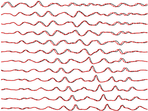
To demonstrate qualitatively the high fidelity of the simulation, snapshots of the normalised measured and simulated free-surface elevation signals are compared at $16$ positions along the wave flume in figure 4. The time window, covering the last $30$ s of the run, is shifted according to probe positions and the local group velocity $C_g(f_p)=\text {d}{\omega }/\text {d}{k}$. It can be seen that the agreement between the simulation and measurements is excellent all over the domain, even after running nearly $90$ min of simulation. Only some minor differences are observed. A small phase shift develops for some waves as they propagate towards the end of the flume: the simulated signal gradually moves ahead of the measurements. This could be explained by the ignored dissipation effect in the simulation: without dissipation, the simulated sea state is of slightly higher energy, with some waves having slightly larger amplitudes. Due to nonlinear dispersion, the phase and group velocities are larger for waves with higher amplitudes, resulting in this small phase shift with the measurements.

Figure 4. Comparison between experimental measurements (black solid lines) and numerical simulation (red dashed lines) of the normalised free-surface elevation recorded at 16 positions along the wave flume (probe positions and the corresponding local relative water depths are indicated above each curve). Each of the time series is shifted vertically with an offset of 10 for the sake of clarity.

2.4. Statistical, spectral and bi-spectral analysis approaches

To analyse the wave transformation processes, four conventional analysis approaches are applied: (i) analysis of characteristic wave parameters, (ii) spectral (Fourier) analysis, (iii) bi-spectral (Fourier-based) analysis and (iv) statistical analysis. Since these analysis techniques are commonly used, the formulations and definitions of notations are reported in appendix A, and we mention below only specific aspects.

Regarding (i), eight non-dimensional parameters are selected to characterise the spatial evolution of the sea state. The nonlinearity is characterised by the normalised significant wave height $H_{m_0}/H_{m_0,inc}$, steepness parameter $H_{m_0}/\hat {L}_p$ (where $\hat {L}_p$ is the wavelength related to the peak frequency $\hat {f}_p$ evaluated with the method of Young (Reference Young1995), see (A3)), skewness $\lambda _3$ and kurtosis $\lambda _4$ of several kinematic variables (free-surface elevation, orbital velocities and accelerations) and the asymmetry parameter computed from bi-spectrum. The subscript ‘inc’ denotes the incident wave characteristic given in table 1. The dispersion parameters include the peakedness parameter $Q_p$, and the normalised local peak frequency $\hat {f_p}/f_{p,inc}$. As a balance of nonlinearity and dispersion, the Benjamin–Feir (B–F) index is considered, with two definitions $\textrm {BFI}_{S06}$ and $B_s$ applicable for different relative depth conditions. The parameter definitions and related formulations are provided in appendix A.1 Regarding (iii), the bi-spectral analysis includes both bi-spectrum $B(f_1,f_2)$ and bi-coherence $b^{2}(f_1,f_2)$. The spectral and bi-spectral analysis approaches are described in appendix A.2 Regarding (iv), the statistical distributions of crest-to-trough wave heights $H$ and free-surface elevation $\eta$ are considered to characterise the deviation of the sea state from Gaussianity. The experimental and simulated distributions are compared with the Gaussian distribution for $\eta$ and the theoretical model of Boccotti (Reference Boccotti2000) for $H$. The distributions of $\eta$ and $H$ are given in appendix A.3.

2.5. Harmonic separation method

In addition, a harmonic separation method is adopted here. The idea of group inversion allows decomposing of the wave group into fundamental components, and was first adopted by Baldock, Swan & Taylor (Reference Baldock, Swan and Taylor1996) to study focused wave groups in deep water. Assuming the time record of, for instance, free-surface elevation or wave-induced load on a structure can be approximated by a Stokes-like harmonic series in both frequency and wave steepness, then the higher-order nonlinear contributions to the time record can be separated by using a so-called ‘phase-inversion’ method. This method requires two tests (either experimental or numerical) using two incident wave trains with identical component amplitudes and frequencies but phases shifted by ${\rm \pi}$. The underlying assumptions of this method are twofold: the existence of a generalised Stokes-type harmonic series expansion in both frequency and wave steepness, and the validity of Stokes's perturbation expansion up to the target order. This method has been applied to study wave–body interactions in uniform water depth (Zang et al. Reference Zang, Gibson, Taylor, Taylor and Swan2006, Reference Zang, Taylor, Morgan, Tello, Grice and Orszaghova2010; Fitzgerald et al. Reference Fitzgerald, Taylor, Taylor, Grice and Zang2014) and shoaling waves on variable bottom profiles (Borthwick et al. Reference Borthwick, Hunt, Feng, Taylor and Stansby2006; Zheng et al. Reference Zheng, Lin, Li, Adcock, Li and van den Bremer2020).

The phase-inversion method is, however, limited by its capacity in distinguishing $n$th and $(n+2)$th-order harmonics in a wave group. Especially at higher orders, the overlap between them could occur over a range of frequencies, and it is difficult to separate them accurately with digital filters. In this study, the harmonic separation is achieved with a generalised phase-inversion method recently introduced by Fitzgerald et al. (Reference Fitzgerald, Taylor, Taylor, Grice and Zang2014), using four phase shifts. The linear primary component and the first three super-harmonics (up to fourth order) can be isolated with linear combinations of four time histories. The method is here applied to the numerical simulations (as experimental time series are available for a single set of phases). These time histories come from four whispers3D simulations with the incident signals having the same amplitudes and frequencies but shifted phases, namely $0$, ${\rm \pi} /2$, ${\rm \pi}$ and $3{\rm \pi} /2$. The linear combinations of time histories and separated harmonics are as follows:

(2.12)\begin{gather} \eta_{1\textrm{st}}=(\eta_0-\eta_{{\rm \pi}/2}^{H}-\eta_{\rm \pi}+\eta_{3{\rm \pi}/2}^{H})/4 = \eta^{(1,1)}+\eta^{(3,1)}+ \textrm{h.o.t.}, \end{gather}

(2.13)\begin{gather}\eta_{2\textrm{nd}}=(\eta_0-\eta_{{\rm \pi}/2}+\eta_{\rm \pi}-\eta_{3{\rm \pi}/2})/4 = \eta^{(2,2)}+\eta^{(4,2)}+ \textrm{h.o.t.}, \end{gather}

(2.14)\begin{gather}\eta_{3\textrm{rd}}=(\eta_0+\eta_{{\rm \pi}/2}^{H}-\eta_{\rm \pi}-\eta_{3{\rm \pi}/2}^{H})/4 = \eta^{(3,3)}+ \textrm{h.o.t.}, \end{gather}

(2.15)\begin{gather}\eta_{4\textrm{th}}=(\eta_0+\eta_{{\rm \pi}/2}+\eta_{\rm \pi}+\eta_{3{\rm \pi}/2})/4 = \eta^{(2,0)}+\eta^{(4,4)}+ \textrm{h.o.t.}, \end{gather}

where the subscripts $0$, ${\rm \pi} /2$, ${\rm \pi}$, $3{\rm \pi} /2$ denote the applied phase shift, the superscript $H$ denotes harmonic conjugate of the signal computed via Hilbert transform. For the separated harmonic components $\eta ^{(m,n)}$ on the right-hand side, the first index $m$ in the superscript denotes the power in amplitude, and the second index $n$ the order of harmonic. The higher-order terms of fifth- and higher-order in amplitude are omitted and represented by ‘h.o.t.’. Note that, in (2.15), both the fourth-order harmonic $\eta ^{(4,4)}$ and second-order difference harmonic $\eta ^{(2,0)}$ appear. As the overlap between these two components is very limited, a simple low-pass filter can be applied to separate them.

3.1. Spatial evolution of wave spectrum

The spatial evolution of measured and simulated wave spectra is shown in figure 5. The area with no measurement between probes 7 ($x =-2$ m) and 8 ($x =-0.95$ m) is intentionally left blank. It can be seen that the measured spectrum in figure 5(a) and the simulated one in figure 5(b) are in good agreement. Both show clearly the enhancement of second-order harmonics in the frequency range $[1.5f_p,2.5f_p]$ over the shallower region. The energy level of the spectral peak at $f_p$ in the measured spectrum is gradually attenuated in space, whereas this level is more or less unchanged in the simulated spectrum. This is speculated to be a consequence of the dissipation which is not considered in our simulation. The dissipation is more effective in the frequency range near the spectral peak than in the high-frequency range. In the LF range $[0,0.5f_p]$ of both simulated and measured spectra, some long waves appear, especially after the up-slope area. The long waves are of slightly higher energy in the simulation, as shown in figure 5(b). As discussed in § 2.3, the long waves observed in both panels (a) and (b) of figure 5 are considered to originate from nonlinear wave–wave interactions. It is therefore considered the slight overestimation of the LF energy in figure 5(b) results from stronger nonlinear interaction due to a more energetic spectral peak in the simulation after the up-slope area.

Figure 5. Colour maps showing the spatial evolution of the variance density spectrum of the free-surface elevation of Run 3 calculated from: (a) measurements and (b) simulation results. The vertical dashed lines indicate the limits of the sloping bottom areas, located at $x=-1.6$, $0$, $1.6$ and $3.2$ m.

In figure 6, a more detailed comparison of the spectra measured at eight positions is shown to demonstrate the spectral evolution along the wave flume. Figure 6(a) shows the wave train propagates over the deeper region with very limited changes in the main part of the spectrum ($0.5f_p < f < 3f_p$), indicating the nonlinear wave–wave interactions are weak in this range. As the wave train propagates in the shallower region, the waves with frequencies higher than $2f_p$ receive energy in a short distance (figure 6b). In figure 6(c), at the half-length of the shallower region ($x=0.8$ m), secondary spectral peaks around $2f_p$ and $3f_p$ manifest. As the wave train approaches the end of the shallower region (from probe 39 to 55), the secondary peaks around $2f_p$ and $3f_p$ are shifted toward lower frequencies. In figure 6(d), the spectrum measured at probe 91 ($x=3.6$ m) has some similarities with the spectrum measured at probe 1 ($x=-2.7$ m), but the secondary peaks close to $2f_p$ and $3f_p$ do not completely vanish. This indicates the spectral changes resulting from a shoaling area are not fully reversible by setting a symmetrical de-shoaling area due to nonlinear effects. The predictions of whispers3D are seen to be very accurate over a wide frequency range for all spectra shown in figure 6.

Figure 6. Comparison of variance density spectra of surface elevation in different areas: (a) the deeper region until the toe of the up-slope; (b) the beginning of the shallower region; (c) the end of the shallower region; (d) the deeper region after de-shoaling. In all of the panels, the solid lines represent measurements, and dashed lines are simulation results.

3.2. Evolution of non-dimensional parameters

In figure 7, the spatial evolution of twelve non-dimensional parameters is shown in eight panels. For all these parameters, the agreement between the experiment and the simulation is excellent. In figure 7(a), the spatial evolution of two normalised significant wave heights corresponding to the components in the frequency ranges $[0,0.5f_p]$ (LF waves) and $[0.5f_p,0.5f_s]$ (short waves) are shown. For the short-wave $H_{m_0}$, small spatial oscillations over the shoal crest can be observed in both experiment and simulation. In the experiment, the $H_{m_0}$ of the short waves is attenuated in the shallower flat region (dark grey zone) but almost holds constant at other locations. The small decrease of $H_{m_0}$ is attributed to the dissipation in the experiment. It is evident that the dissipation is related to the relative water depth, so we speculate that the dissipation in the experiment was mainly induced by friction on the bottom and sidewalls. The $H_{m_0}$ for LF waves keeps its low level over all the domain. In figure 7(b), a similar pattern of oscillation of the steepness parameter in the shallower flat region as for $H_{m_0}$ is observed. The increase of the steepness parameter over the up-slope is more pronounced than that of $H_{m_0}$, since the local peak wavelength is reduced due to shoaling.

Figure 7. Spatial evolution of non-dimensional wave parameters in measurements ($*$) and in simulations (solid lines) of R3. The light grey zones indicate the sloping areas and the dark grey zone indicates the shallower flat region. In panel (h), the vertical dash lines denote the positions where the threshold $k_ph=1.363$ for modulational instability is achieved.

In figure 7(c), the evolution of the skewness of the free-surface elevation $\lambda _3(\eta )$ and the horizontal velocity $\lambda _3(u(z_0))$ show similar increasing and decreasing trends over the domain. Their maximum and minimum values are achieved roughly at the same positions, both located shortly after the change of bottom gradient (maximum at $x \approx 0.6$ m, and minimum at $x \approx 2.3$ m). The skewness indicates the asymmetry of the probability distribution of the considered variable. For $\eta$, a positive skewness indicates waves with sharper crests and flatter troughs, and vice versa for negative values. According to $\lambda _3(\eta )$, the wave profile is nearly symmetric in the first deeper region and becomes asymmetric with positive skewness over the shallower region. As the wave propagate over the down-slope area, the asymmetry of the wave profile is rapidly inverted. The evolution is similar for the profile of $\lambda _3(u(z_0))$.

In figure 7(d), the values of $\lambda _4(\eta )$ in both experiment and simulation are slightly larger than 3 before the bar. Then, they rapidly increase in the area close to the end of the up-slope, achieving their maxima at the same position as for the skewness. The length of latency is found to be approximately half of the peak wavelength in the shallower region. Then, $\lambda _4(\eta )$ decreases mildly in a larger area, and eventually goes back to 3 around the end of the domain. No particular change of $\lambda _4(\eta )$ is observed in the de-shoaling area. The evolution trend of $\lambda _4(\eta )$ is well captured by the numerical model, although the maximum value of $\lambda _4(\eta )$ is slightly underestimated by $6\,\%$. As was observed in TRJR20, $\lambda _4(u(z_0))$ exhibits a very different behaviour: it does not show any noticeable enhancement over the up-slope area nor over the bar crest, but reaches its maximum value after a short distance in the de-shoaling area. Such behaviour of $\lambda _4(u(z_0))$ is well simulated, including its maximum value.

In figure 7(e), the evolution of the asymmetry parameter is shown. Positive values indicate that, in general, waves are leaning toward the wave-propagation direction, whereas negative values indicate waves are leaning to the opposite direction. The evolution of the asymmetry parameter indicates that the incident waves are almost symmetrical in the horizontal direction for $x<-1$ m. As waves propagate over the bar, the general wave profile leans backward first, and then forward. The most backward-leaning wave profile is achieved in the shallower flat region, and the most forward-leaning profile in the de-shoaling area. We note the largest asymmetry of the sea state in horizontal direction is achieved before $\lambda _3(\eta )$ takes its maximum and minimum values. This implies the deformations of wave shape in horizontal and vertical directions are largely independent.

Figures 7(f) and 7(g) show that $Q_p$ and $\hat {f_p}$ evolve in an oscillatory manner until the end of the shallower region. After that, the changes of these two parameters are very limited. The evolution of $Q_p$ is remarkably well simulated (figure 7f). For $\hat {f_p}$ in figure 7(g), the agreement between the experiment and simulation is also good. The peak frequency is only underestimated, by a few per cent at most, in the simulation. By and large, the spectral changes in terms of the spectral width and peak frequency are quite limited.

In figure 7(h), the spatial evolution of the two forms of the B–F index (A5) and (A12) is shown in logarithmic scale. In the present case, the threshold $k_ph=1.363$ for modulation instability is achieved at $x=-0.95$ and $2.55$ m. At these two positions, two forms of the B–F index take $0$ because the coefficient $\sqrt {{|\beta |}/{\alpha }}=0$ at this threshold relative water depth (see the expressions of $\alpha$ and $\beta$ in (A8) and (A9)). Between these abscissae, waves are expected to be modulationally stable, both $\textrm {BFI}_{S06}$ and $B_s$ no longer indicate the significance of modulation instability but only characterise the relative importance of nonlinearity and dispersion. Both formulations show significant variations over the up- and down-slopes with similar spatial profiles. The variations of $\textrm {BFI}_{S06}$ and $B_s$ in the modulationally stable area are large compared to those in the unstable area. Such a significant difference is also due to the property of the coefficient $\sqrt {{|\beta |}/{\alpha }}$. It monotonically increases from $0$ to $1$ for $k_ph \geqslant 1.363$, but increases exponentially as $k_ph$ decreases from $1.363$ to $0$. The magnitude of $B_s$ is higher than that of $\textrm {BFI}_{S06}$ over the shallower region, due to the correction of the wave-induced mean flow. In line with the evolution of $H_{m_0}$ and steepness parameter, the evolution trend changes right after the transition points of bottom gradient for the B–F index. This means the change of nonlinearity due to depth variations is more significant than that of the dispersion, and the changes stop immediately when waves enter flat bottom regions.

3.3. Bi-spectrum and bi-coherence

Bi-spectral analysis of $\eta$ time series allows the gaining of insight into nonlinear wave coupling between modes. In figures 8 and 9, we show the bi-coherence for the relative strength of nonlinear coupling and the imaginary part of the bi-spectrum for the energy transfer direction, in the area from $0.25$ m to $1.3$ m (over the shallower region). In this area, the skewness and kurtosis vary significantly, with their maximum values achieved at $x \approx 0.6$ m. This indicates that the most active nonlinear interaction takes place in this area. Each panel contains the bi-spectrum from measurements in the lower right triangle and the bi-spectrum from simulation in the upper left triangle (so that the agreement between them can be estimated from the symmetry about the line $f_1=f_2$).

Figure 8. Contours of bi-coherence over the shallower region at eight probe positions between $x=0.25$ m (probe 28) and $x=1.3$ m (probe 49), in (a) simulated results; (b) measurements. The probe numbers and positions are indicated in each panel, together with the corresponding maximum bi-coherence values.

Figure 9. Contours of the imaginary part of the bi-spectrum over the shallower region at eight probe positions between $x=0.25$ m (probe 28) and $x=1.3$ m (probe 49), in (a) simulated results; (b) measurements. The probe numbers and positions are indicated above each panel.

From the evolution of the bi-coherence $b^{2}$ shown in figure 8, we note the strongest interaction always takes place in the region near the spectral peak. The strongest coupling, achieved at $b^{2}(1.01f_p,1.01f_p)$, reflects intense energy transfer among $f_1=1.01f_p$, $f_2=1.01f_p$ and $f_1+f_2=2.02f_p$. This interaction corresponds to the development of the second harmonics around $2f_p$ in the spectrum. A less strong but clearly visible interaction takes place around $b^{2}(2f_p,f_p)$, which becomes increasingly significant as waves propagate from $x=0.25$ m to $1.3$ m. It corresponds to the development of the third harmonics around $3f_p$. More generally, we notice the non-zero bi-coherence in the range between $b^{2}(f_p,f_p)$ and $b^{2}(2f_p,f_p)$ from probe 28 to 34, which indicates that the harmonics with frequencies $2f_p\leqslant f \leqslant 3f_p$ are involved in the interactions. This is in agreement with the observations in figure 6(b), where a clear increase is noticed for the whole tail of the spectrum above $2f_p$ at probe 31. After some distance, non-zero values of $b^{2}$ appear only around $b^{2}(f_p,f_p)$ and $b^{2}(2f_p,f_p)$ resulting in the formation of second and third harmonics. In the simulation, not only the components of the nonlinear interactions but also the levels of bi-coherence are well predicted for the listed probes.

In figure 9, the energy transfer direction can be inferred, by considering the imaginary part of the bi-spectrum. Positive values indicating sum interactions are represented by colours from green to red. Meanwhile, negative values indicating difference interactions are represented by green to blue. It is clearly seen that the sum interactions first take place over the first half of the shallower flat region (from probe 28 to 34), forming the second harmonics around $2f_p$. Close to the centre of the shallower region, at probes 37 and 40, difference interactions appear around $(f_p,f_p)$, indicating energy transfer from the second harmonics $2f_p$ back to the $f_p$ mode. In this area, both the sum and difference interactions are present. As waves approach the second half of the shallower region (from probe 43 to 49), difference interactions dominate. Besides, difference interactions are present around $\textrm {Im}{\{B(f_p,0.25f_p)\}}$. This indicates energy transfer from the frequency $1.25f_p$ to $f_p$ and $0.25f_p$, thus the generation/enhancement of LF waves with frequency $0.25f_p$. In general, the agreement between simulation and experiment is very good. Only some small differences can be observed in the LF range, which explain the overestimation of LF energy in the simulated spectrum in figure 5(b).

3.4. Harmonic analysis

The application of the generalised phase-inversion method outlined by Fitzgerald et al. (Reference Fitzgerald, Taylor, Taylor, Grice and Zang2014) requires moderate nonlinearity of the sea state, in order to adopt a Stokes-type harmonic series to represent the time series of $\eta$. As wave nonlinearity is significantly enhanced due to shoaling, attention should be paid to the applicability of this approach in the current case. To evaluate the applicability of the harmonic separation technique in the present case, the sea state is represented by the so-called first-, second- and third-order harmonics. These characteristic waves are of frequencies $f_p$, $2f_p$ and $3f_p$ respectively, and their representative wave heights are computed in the same way as for the significant wave height but over different frequency ranges, namely $[0.5f_p,1.5f_p]$, $[1.5f_p,2.5f_p]$ and $[2.5f_p,3.5f_p]$. The representative frequencies and wave heights are computed locally and averaged over the areas with constant depth $h_1$ and $h_2$. In figure 10, the representative harmonics are placed in the diagram of Le Méhauté (Reference Le Méhauté1976). It is seen the first three harmonics fall in the range of validity of Stokes second-order theory in both flat regions: the harmonic separation method is thus applicable.

Figure 10. Le Méhauté's diagram (Le Méhauté Reference Le Méhauté1976), with the first three representative harmonics of the irregular wave train of R3 added.

After running three additional simulations with ${\rm \pi} /2$, ${\rm \pi}$ and $3{\rm \pi} /2$ phase shifts for the incident wave train, the contributions of harmonics at different orders $\eta _{1\textrm {st}}$, $\eta _{2\textrm {nd}}$, $\eta _{3\textrm {rd}}$, $\eta _{4\textrm {th}}$ to the original time record of $\eta$ can be evaluated from (2.12)–(2.15). The spatial evolution of their spectra is shown in figure 11. It can be seen that the different harmonics have been successfully extracted. The spectrum of the primary components (figure 11a) evolves with nearly no modulation over the domain. Figure 11(b) indicates the increase of energy around $2f_p$ is mainly due to second-order sum interactions. In figure 11(c), the third harmonic is seen to be weak except over the bar crest. In figure 11(d), showing $\eta _{4\textrm {th}}$, two components $\eta ^{(4,4)}$ and $\eta ^{(2,0)}$ should be present according to (2.15). However, the fourth harmonic $\eta ^{(4,4)}$ is weaker than the lower bound of the current colour scale, with negligible contribution here. Therefore $\eta _{4\textrm {th}} \approx \eta ^{(2,0)}$, showing the role of second-order difference interactions in driving the energy increase of LF waves.

Figure 11. Spatial-spectral evolution of extracted harmonics at different orders (in logarithmic scale): (a) the first-order component $\eta _{1\textrm {st}}$, (b) the second-order component $\eta _{2\textrm {nd}}$, (c) the third-order component $\eta _{3\textrm {rd}}$ and (d) the fourth-order component $\eta _{4\textrm {th}}$. The vertical dashed lines indicate the limits of the sloping bottom areas, located at $x=-1.6$, $0$, $1.6$ and $3.2$ m.

We note that Zheng et al. (Reference Zheng, Lin, Li, Adcock, Li and van den Bremer2020) applied this technique using the phase-inversion approach (i.e. with two time series $\eta$ and $\eta _{{\rm \pi} }$), resulting in the separation of $(\eta _{1\textrm {st}}+\eta _{3\textrm {rd}})$ and $(\eta _{2\textrm {nd}}+\eta _{4\textrm {th}})$, denoted as $\eta _{odd}$ and $\eta _{even}$ respectively. Clearly, the two separated components $\eta _{odd}$ and $\eta _{even}$ would be subject to some overlap. In the present work, the generalised (four-phase) phase-inversion method permits us to isolate the first four harmonics with good quality.

Based on this decomposition, we analyse the contribution of the four harmonics to the changes of skewness and kurtosis by considering cumulative summations of the separated signals (figure 12). In (a), the skewness of the primary component is nearly 0. By adding the contribution due to the second-order sum interaction, $\lambda _3(\eta _{1\textrm {st}}+\eta _{2\textrm {nd}})$ is significantly enhanced, showing very similar variations in space as $\lambda _3(\eta )$. The second harmonic thus dominates the changes of skewness over the entire domain. Although $\eta _{3\textrm {rd}}$ makes little contribution to the spectrum, see figure 11(c), it affects skewness evolution in a non-negligible way. Furthermore, the effects of $\eta _{3\textrm {rd}}$ appear only in the area where the sea state is out of equilibrium, namely, starting shortly after the up-slope and ending shortly after the shallower flat region. We note $\lambda _3(\eta _{1\textrm {st}}+\eta _{2\textrm {nd}}+\eta _{3\textrm {rd}})$ is larger than $\lambda _3(\eta )$, indicating that the LF components due to second-order difference interactions are responsible of a decrease of skewness.

Figure 12. Spatial evolution of (a) skewness and (b) kurtosis of the time series of $\eta$ obtained from the simulation of the R3-bar case without phase shift, and different combinations of separated time series (see legend).

In figure 12(b), it is observed that the kurtosis of the primary component becomes lower than $3$ as water depth decreases. The second harmonic component, $\eta _{2\textrm {nd}}$, affects the kurtosis over the entire domain, with an evident enhancement over the bar crest. The inclusion of $\eta _{3\textrm {rd}}$ significantly enhances the kurtosis over the same area as for skewness. Again, the contribution of bound LF waves $\eta _{4\textrm {th}}$ results in a decrease of kurtosis. Based on these observations, it is anticipated that the changes of skewness and kurtosis due to shoaling are related to both second- and third-order nonlinear interactions in the current case, and the non-equilibrium dynamics is associated with third-order effects, resulting in significant enhancement of kurtosis.

3.5. Statistical distributions

In figure 13, the probability density functions (PDFs) of the $\eta$ time series at $6$ probes over the bar are shown, with the Gaussian PDF superimposed as a reference. The measured and simulated PDFs show excellent agreement for all the probes shown. In the experiment, the sea state remains quasi-Gaussian until the end of the up-slope (probe 23). Over the bar crest (from probe 23 to probe 55), strong deviations from Gaussianity manifest. The positive tail of the distribution is shifted toward higher values of $\eta /\sqrt {m_0}$, indicating that the highest wave crests are noticeably larger in comparison with the Gaussian prediction. Meanwhile, the negative tail is shifted toward lower values, indicating the wave troughs are shallower. Such observations are in agreement with the expectation of positive skewness in this area. Among all the positions shown here, the strongest non-Gaussian behaviour takes place close to the middle of the shallower region (probes 35 to 39), at the length of latency. At the end of the bar crest (probe 55), the deviation of the empirical PDF from the Gaussian one decreases. This is related to the effects of de-shoaling and the weakening of the non-equilibrium dynamics. This is also in agreement with the indication of bi-spectral analysis, from which we found energy transfer from the second harmonic $2f_p$ back to the peak frequency $f_p$, and a decrease of nonlinear interactions. Eventually, at the end of the de-shoaling zone (probe 87), the empirical PDF turns back to Gaussian.

Figure 13. PDF of free-surface elevation ($\eta$) at $6$ probe positions between $x=-0.8$ m (probe 9) and $x=3.2$ m (probe 87). The probe numbers and positions are indicated above each panel. The Gaussian distribution is superimposed to highlight the nonlinear characteristics of the sea state.

In figure 14, the complementary cumulative distribution functions (CCDFs) of wave height $H$ are shown at the same positions as in figure 13, with the distribution of Boccotti (Reference Boccotti2000) superimposed as reference. Again, the agreement between the simulation and measurements is excellent, even in the tail of the distributions. Only few of the largest waves are slightly higher in the simulation at probes 39 and 55. Starting as a quasi-Gaussian process at probes 9, the sea state undergoes a clear deviation from Gaussianity as waves propagate over the bar crest, with a marked increase of large waves, in particular at probes 35 and 39, and to a lesser extent until the end of this area (probe 55). Over the bar crest, and in particular in the zone $0.5\ \textrm {m} < x < 1\ \textrm {m}$, several ‘freak waves’ can be identified based on the criterion $H>2H_{m_0}$. The distribution of Boccotti (Reference Boccotti2000) predicts that the occurrence probability of waves with $H>2H_{m_0}$ is lower than 0.01 % (the lower limit of the $y$-axis in figure 14). In agreement with the increase of $\lambda _4(\eta )$ discussed previously (see figure 7(d) or 12(b)), these wave height distributions clearly demonstrate the increase of the occurrence probability of freak waves due to the water depth transition. At the end of the de-shoaling area (probe 87), where the PDF of $\eta$ is very close to Gaussian in figure 13, the empirical CCDF of $H$ is lower than the theoretical prediction in the high-wave range. We note the CCDF of $H$ at probe 87 is rather close to the distribution observed before the bar crest (probe 9), with a reduction of the occurrence probability of large waves. This is again considered to be an effect of the de-shoaling process.

Figure 14. CCDF of wave height ($H$) at $6$ probe positions between $x=-0.8$ m (probe 9) and $x=3.2$ m (probe 87). The probe numbers and positions are indicated above each panel. The vertical dashed line in each panel represents the commonly adopted threshold for freak waves: $H=2H_{m_0}$.

3.6. Statistics of velocity and acceleration

In the R3 experiment, the horizontal velocity at $z_0=-0.048$ m has been measured at 37 positions, and studied statistically in TRJR20. In § 3.2 we have shown the skewness and kurtosis of $u(z_0)$ simulated with whispers3D are in excellent agreement with the measurements (see figure 7c,d). Here, using additional model results, we present a more complete statistical analysis of the kinematic properties, namely the vertical velocity and accelerations in both directions. The local (Eulerian) horizontal and vertical accelerations, denoted as $u_t(z_0)$ and $w_t(z_0)$ respectively, are evaluated as time derivatives of $u(z_0)$ and $w(z_0)$. The computation of derivatives is made with a five-point centred finite difference scheme. In the following, we analyse the spatial evolution of the skewness and kurtosis of 5 variables: $\eta , u(z_0), w(z_0), u_t(z_0), w_t(z_0)$.

In figure 15(a), the evolution of skewness of the five kinematic variables is plotted. Two groups of variables can be identified, showing two different spatial evolution patterns. First, we note $\lambda _3(w(z_0))$ and $\lambda _3(u_t(z_0))$ evolve very closely over the whole domain. They both reach two local maximum and one local minimum values, at almost the same positions for both variables (first maximum at $x\approx 0.2$ m, minimum at $x \approx 1.9$ m, second maximum at $x \approx 2.6$ m). In addition, it is noticed that the profile of the asymmetry parameter in figure 7(c) is similar to that of $\lambda _3(w(z_0))$ and $\lambda _3(u_t(z_0))$, despite an opposite sign. In the second group, the spatial profiles of $\lambda _3(\eta )$, $\lambda _3(-w_t(z_0))$ and $\lambda _3(u(z_0))$ present a lot of similarities, although with different magnitudes. The local maximum and minimum values of skewness of these three variables are located downstream compared to the ones of $w(z_0)$ and $u_t(z_0)$. The skewness of $w_t(z_0)$ shows the most pronounced variation, with its global maximum achieved around $x=0.45$ m. The skewness of $u(z_0)$ shows a lower minimum value in the middle of the down-slope area (around $x=2.3$ m). The spatial profiles of the skewness of these five variables and the asymmetry parameter indicate that the adaptation of the sea state due to depth variations has different impacts on kinematic properties, among which two dominant typical evolution patterns can be identified.

Figure 15. Spatial evolution of (a) skewness and (b) kurtosis of five variables obtained from the simulation of the R3-bar case: free-surface elevation $\eta$, horizontal and vertical velocities $u$, $w$, horizontal and vertical accelerations $u_t$, $w_t$. The velocities and accelerations are computed at the same elevation $z_0=-0.048$ m.

It is known from linear theory that $\eta , u$ and $-w_t$ are of the same phase in a linear superposition of progressive harmonic components, while $w$ and $u_t$ are also in phase, but with a phase shift of ${\rm \pi} /2$ with respect to the variables of the former group. In the nonlinear case, such an expectation is not guaranteed a priori. The observations in figure 15(a) indicate that the phase relations among the five variables are somewhat preserved in the present case.

Figure 15(b) shows the kurtosis evolution of the same variables. As was observed in TRJR20, $\lambda _4(u(z_0))$ shows no sign of enhancement over the up-slope or the bar crest, whereas a local maximum is achieved in the down-slope area. This trend is successfully captured in the simulation. However, model results show that $\lambda _4(w(z_0))$, $\lambda _4(u_t(z_0))$ and $\lambda _4(-w_t(z_0))$ (not discussed in TRJR20) are noticeably enhanced over the shallower region, with their maximum values achieved at the same position (approximately $x=0.6$ m, corresponding to the length of latency) as for $\lambda _4(\eta )$. Regarding the variables $u_t(z_0)$ and $w(z_0)$, we note that their kurtosis profiles are very similar, as was observed for their skewness profiles in figure 15(a). The value of $\lambda _4(-w_t(z_0))$ shows the most significant enhancement over the bar crest with only one maximum in the domain, as for $\lambda _4(\eta )$. Our results supplement the observations made on $\lambda _4(u(z_0))$ in TRJR20, showing that significant changes of kurtosis of other kinematic properties, namely $w(z_0)$, $u_t(z_0)$ and $-w_t(z_0)$, take place due to depth variations. Furthermore, the kurtosis profiles of these 3 variables are markedly different from the one of $u(z_0)$. All three show a significant increase of kurtosis over the bar crest (implying an increased occurrence probability of their maximum values), in line with the increase of $\lambda _4(\eta )$ in this area.

4.1. Objectives and outline of the simulation with a step-like profile

In § 3, an extensive analysis of the effects induced by wave shoaling in the up-slope area has been performed, together with the effects of the down-slope (de-shoaling). At the up-slope transition, the out-of-equilibrium dynamics of the wave train is associated with the spectral settling from the deeper-water equilibrium state (in depth $h_1$) to the shallow-water equilibrium (in depth $h_2$), and this process takes place over a certain distance after the start of the shallower region. However, this shallower-water area is of relatively short length in the R3-bar set-up. One may wonder whether the out-of-equilibrium dynamics due to up-slope transition has been fully developed in the shallower region and what is the contribution of the de-shoaling process. The sea state could enter the de-shoaling area before having reached a new shallow-water equilibrium, it is therefore difficult to conclude which effects govern the sea-state dynamics after the shallower region.

In order to isolate the effects of the two slopes and to better assess the characteristic distance of non-equilibrium dynamics due to the shoaling process, an additional simulation without the de-shoaling area has been conducted with a modified bathymetry profile (R3-step set-up in figure 2b). The simulation of the new case is conducted with the same numerical parameters as for the R3-bar case. In this section, we show the results of this new R3-step case, and compare them with those of the R3-bar case. We focus on the spatial evolution of the variance density spectrum (§ 4.2), non-dimensional parameters (§ 4.3) and the statistics of the kinematic variables (§ 4.4).

4.2. Spatial evolution of wave spectrum

In figure 16, the spectral evolution in space shows the wave spectra of the two set-ups exhibit very similar patterns in the area where the bottom profiles are identical ($x < 1.6$ m). After $x=1.6$ m, the differences in the spectra manifest mainly for two frequency ranges: $f>1.5f_p$ and $f<0.5f_p$. In the R3-step case, more energy is transferred to components in these two ranges, which is clearly the consequence of stronger nonlinear interactions in the extended shallower region. In figure 16(b) for the R3-step case, a second energetic peak around $2f_p$ appears after $x \approx 2.5$ m and lasts until the end of the domain.

Figure 16. Spatial evolution of the variance density spectra in simulations (a) with the R3-bar set-up, and (b) with the R3-step set-up. The vertical dashed lines indicate the limits of the sloping bottom areas in the R3-bar set-up, located at $x=-1.6$ m, $0$ m, $1.6$ m and $3.2$ m. The solid black curves in panel (b) represent the predicted maximum values of the spectral amplitude, between which the distance in space corresponds to the beating length of the second harmonics of primary frequencies in $[0.8f_p,1.5f_p]$.

In the area from $x=1.6$ m to $3.6$ m, there is a particular spatial evolution of the spectrum for $f > 1.6f_p$, quite different from the R3-bar case. It is believed this particular spatial structure in the high-frequency range is due to the simultaneous presence of free and bound components with frequencies being higher harmonics of frequencies close to the spectral peak (typically in the range $[0.8f_p,1.5f_p]$). This situation is typically encountered when waves propagate over a submerged bar or shoal (Beji & Battjes Reference Beji and Battjes1993) or when waves are generated using a wave shape that does not correspond to the stable form of progressive nonlinear waves for the considered depth (Chapalain, Cointe & Temperville Reference Chapalain, Cointe and Temperville1992). As is well known, if free and bound components at a higher harmonic $Nf$, with $N=2,3,\ldots$, of the primary frequency $f$ coexist in constant depth, a beating or spatial modulation of the amplitude will manifest. This effect is most apparent here for the second harmonics ($N=2$) of the primary frequencies $f \in [0.8f_p,1.5f_p]$. The beat length of the second harmonics, defined as the distance between two successive maximum values of the spectral amplitude, can be estimated following Massel (Reference Massel1983)

(4.1)\begin{equation} L_{beat}(2f)=\frac{2 {\rm \pi}}{k(2f)-2k(f)}, \end{equation}

where the wavenumbers $k(f)$ and $k(2f)$ are computed from $f$ and $2f$ using the linear dispersion relation (for depth $h_2$). Following this idea, the beating lengths of the second harmonics for $f \in [0.8f_p, 1.5f_p]$ have been computed and superimposed in figure 16(b). The estimation of the beating length for $f \in [0.8f_p, 1.5f_p]$ results in a series of curves in the range $[1.6f_p, 3f_p]$ as second harmonics. The distance between two successive curves at a particular frequency corresponds to the beating length. These curves are in good agreement with the spatial modulations of the spectrum in figure 16(b) for $f>1.6f_p$.

In the R3-bar case (figure 16a), this effect is less pronounced due to the variable depth over the down-slope area, but is still visible for $f > 2f_p$. It is also noted that, for the case of a larger (uniform) depth in (4.1), the beat length would be reduced. This reduction does not appear clearly after the down-slope area in figure 16(a). This is because the area with constant deeper water ($h_1=0.53$ m) after $x=3.2$ m is only $0.4$ m long, which is less than the shortest beating length $L_{beat}(3f_p) \approx 0.42$ m in the considered frequency range $[0.8f_p, 1.5f_p]$. However, comparing the spectra of two simulations in the range $x>1.6$ m and $f/f_p>2$, some indication of this reduction can be detected in figure 16(a), although the depth is not uniform from $x=1.6$ m to $3.2$ m in the R3-bar case. In summary, the water depth reduction due to the up-slope results in an increase of wave nonlinearity in the shallower area, which manifests in the forms of energy transfer, generation of bound long waves and increase of the amplitude of the bound super-harmonics of the frequencies near the spectral peak. In addition, as the depth variation is rather abrupt, part of the energy is also transferred to free waves in the same high-frequency range, resulting in the above-described spatial modulation of spectrum magnitude.

In figure 17, the comparison of the spectra in two simulations is shown at four positions after $x=1.6$ m. At $x=1.6$ m (figure 17a), the main parts of the two spectra are superimposed. As waves propagate in the extended shallower region in the R3-step case, differences gradually manifest in figure 17(b–d). In the R3-step case, the harmonic peak around $2f_p$ is more pronounced in comparison with the R3-bar case, and we notice this peak is gradually shifted from frequencies slightly higher than $2f_p$ to lower frequencies. We also note the spectrum tail in the range $[2.5f_p,4f_p]$, which is decreased in the R3-bar case, is preserved in the R3-step case. This indicates that the de-shoaling process results in a loss of energy of the high-frequency waves. The LF waves receive more energy in the R3-step case due to stronger nonlinear interactions in the extended shallower region for $x>1.6$ m. In the R3-bar case, the spectral evolution in figure 17(b–d) is quite limited. It indicates that the spectral adaptation to the shallow-water equilibrium was not fully developed over the $1.6$ m long bar crest in the R3-bar case, and was balanced by the de-shoaling process.

Figure 17. Comparison of spectra of the surface elevation at 4 positions from numerical simulations for the R3-step (solid lines) and the R3-bar (dashed lines) cases.

4.3. Non-dimensional parameters

Figure 18 compares the spatial profiles of twelve non-dimensional parameters for the R3-bar and R3-step cases. In figure 18(a), the small spatial modulations of $H_{m_0}/H_{m_0,inc}$ calculated in the main frequency range $[0.5f_p,0.5f_s]$ disappear over the shallower region in the R3-step case. This indicates that the de-shoaling process can influence the upstream wave field, possibly via the generation of reflected free waves. Similar trends can be found for the evolution of the steepness parameter, $Q_p$, and $\hat {f}_p/f_p$. In the R3-step case, the $H_{m_0}$ of the LF range keeps increasing in the extended shallower region. Due to strong nonlinear interactions in this region, wave energy is continuously transferred toward these sub-harmonic components. In figure 18(b), the decrease of the steepness parameter for $x>1.6$ m disappears in the R3-step case, because $\hat {L}_p$ remains uniform in the extended shallower region.

Figure 18. Spatial evolution of non-dimensional parameters in simulations of the R3 case with de-shoaling area (dashed lines), and without de-shoaling area (solid lines). The light grey zones indicate the sloping areas and the dark grey zone indicates the shallower flat region in the case with the de-shoaling area. In panel (h), the vertical dashed lines denote the positions where the threshold $k_ph=1.363$ for modulational instability is achieved.

In figure 18(c–e), significant discrepancies of skewness, kurtosis and asymmetry parameters from the results of the R3-bar case are observed for $x>1.6$ m. In the R3-step case, these parameters are seen to converge toward new constant levels in the extended shallower region, after reaching their maximum/minimum values over the original shallower region. This is an indication that the sea state is evolving toward a new equilibrium state in the shallower region, since the effects of the non-equilibrium dynamics induced by the up-slope gradually decrease in space. In the range $x<1.6$ m, where both profiles are identical, these statistical parameters are almost superimposed. We thus conclude that the local minimum values of $\lambda _3(\eta )$ and $\lambda _3(u(z_0))$, the local maximum value of $\lambda _4(u(z_0))$ and the variations of the asymmetry parameter, observed for $x>1.6$ m in the R3-bar case (see figure 7c,d), are caused by de-shoaling effects. This is of interest for interpreting the particular behaviour of $\lambda _4(u(z_0))$ highlighted in figure 7(d): the local maximum of $\lambda _4(u(z_0))$ is not due to the up-slope transition, but to the down-slope one. In the R3-step case, $\lambda _4(u(z_0))$ shows nearly no variation over the whole domain, in contrast to $\lambda _4(\eta )$ that experiences strong enhancement in the first part of the shallower region.

Figures 18(f) and 18(g) show the comparison of $Q_p$ and $\hat {f}_p/f_p$, respectively. For these parameters, the differences between the two set-ups are not restricted to the de-shoaling area but also manifest in the area where the two bottom profiles are identical. The spatial modulations of $Q_p$ and $\hat {f}_p/f_p$ seen in the R3-bar case for $x < 1.6$ m become insignificant in the R3-step case. As explained above, this indicates that de-shoaling affects not only the wave field in the area after the beginning of the down-slope but also the upstream wave field (reflected waves). Besides this difference, both cases show another modulation of $Q_p$ and $\hat {f}_p/f_p$ before entering the shallower region (i.e. for $x<0$) attributed to the reflection of incident waves on the up-slope part. In summary, this comparison highlights the fact that the spatial modulations of $Q_p$ and $\hat {f}_p/f_p$ observed in the R3-bar case before $x=1.6$ m originate from two reflection processes taking place at the up-slope transition (in both cases), and at the down-slope transition (in the R3-bar case only).

Figure 18(h) shows that the $\textrm {BFI}_{S06}$ and $B_s$ parameters in the R3-step case are almost superimposed with the ones in the R3-bar case for $x<1.6$ m. However, no decrease after $x=1.6$ m is seen in the R3-step case, due to the extended shallower region.

4.4. Statistics of velocity and acceleration

Figure 19 compares the spatial profiles of skewness (a) and kurtosis (b) of the kinematic properties in the two simulations. In the R3-step case, the skewness of all the kinematic properties continue their decreasing or increasing trend over a short distance in the extended shallower region. This is because the non-equilibrium dynamics induced by the up-slope keeps having effects after $x=1.6$ m. After a short distance in the extended shallower region, the variations of skewness in the R3-step case become mild. But it is evident that the steady shallow-water state has not been established yet, even in the R3-step case. As evidence, $\lambda _3(u(z_0))$ keeps its increasing trend until the end of the flume. Based on the observations in Zhang et al. (Reference Zhang, Benoit, Kimmoun, Chabchoub and Hsu2019), where a long shallower region was used, we anticipate that the mild modulation of skewness in the R3-step case would continue over a longer distance without significant changes if the flume was extended. The skewness differences between the two bottom set-ups correspond to the de-shoaling effects, and it is clear that the de-shoaling process results in opposite effects to the skewness compared to shoaling. The sharp decrease of skewness after $x=1.6$ m is mainly due to de-shoaling effects (rather than the decrease of up-slope induced non-equilibrium dynamics). It is also noticed that the de-shoaling process slightly influences $\lambda _3(u(z_0))$ and $\lambda _3(\eta )$ before the down-slope area. Regarding skewness, the most sensitive variable to the change of water depth is $w_t$.

Figure 19. Spatial evolution of (a) skewness and (b) kurtosis of five variables $\eta$, $u(z_0)$, $w(z_0)$, $u_t(z_0)$ and $-w_t(z_0)$ in both the R3-bar and R3-step cases.

In line with the observations for skewness, figure 19(b) shows the kurtosis of the five variables continue their decreasing trend over a short distance in the extended shallower region in the R3-step case. This is due to the weakening of the non-equilibrium dynamics. The differences of kurtosis between the R3-step and R3-bar cases again correspond to the de-shoaling effects. Unlike skewness, both shoaling and de-shoaling processes result in the enhancement of kurtosis. Since kurtosis involves the mean of an even power of a variable, it does not distinguish, for instance, a deep trough (negative) from a sharp crest (positive) for $\eta$. It should be noticed that the effects of the de-shoaling process on the spatial evolution of the kurtosis are different for the five variables. No significant enhancement of $\lambda _4(-w_t(z_0))$ and $\lambda _4(\eta )$ is observed in the R3-step case. On the contrary, the kurtosis of $u_t(z_0)$, $w(z_0)$, $u(z_0)$ is increased in the extended shallower region of the R3-step case. Combined with the behaviour of the skewness for these variables in the same region, we know that the increase of kurtosis is due to more negative extreme values (velocity or acceleration in the direction toward bottom). Regarding kurtosis, the most sensitive variable to the depth variation is again $w_t(z_0)$, whereas $\lambda _4(u(z_0))$ shows almost no change over the domain in the R3-step case.