2.1 Detection of the turbulent/non-turbulent interface

The turbulent/non-turbulent interface (TNTI) that demarcates the turbulent and non-turbulent regions can be defined based on kinetic energy criteria (Chauhan et al. Reference Chauhan, Philip, De Silva, Hutchins and Marusic2014). The purpose of this section is to introduce the contamination of velocity fluctuations by using the Reynolds decomposition near the TNTI. The accurate prediction of the TNTI is important for extracting wall-attached clusters in the outer region. The wall-normal height of the TNTI $\unicode[STIX]{x1D6FF}_{TNTI}(x,z,t)$ is varied depending on the boundary layer thickness $\unicode[STIX]{x1D6FF}(x)$. As a result, the structures of velocity fluctuations are contaminated near the TNTI (Kwon, Hutchins & Monty Reference Kwon, Hutchins and Monty2016). In particular, both large and small scales near the TNTI are significantly amplified in the APG TBL. The raw streamwise velocities ($\tilde{u}$) normalized by $U_{\infty }$ are displayed in figure 2(ai), where the white line is the contour $\tilde{u} /U_{\infty }=0.95$. Figure 2(aii) shows the logarithm of the local kinetic energy (k) obtained from all velocity fluctuations in the reference frame moving with $U_{\infty }$ over $3\times 3\times 3$ grids, and the black line in figure 2(aii) indicates the threshold value of $k$ chosen at $k_{threshold}=0.2$, which corresponds closely to the line $\tilde{u} /U_{\infty }=0.95$. The red line in figure 2(aiii) shows the TNTI determined from the black $k_{threshold}$ line. The mean height of the TNTI is $\langle \unicode[STIX]{x1D6FF}_{TNTI}\rangle =0.9\unicode[STIX]{x1D6FF}$, which is slightly higher than that of a ZPG TBL $(\langle \unicode[STIX]{x1D6FF}_{TNTI}\rangle =0.88\unicode[STIX]{x1D6FF})$ (Hwang & Sung Reference Hwang and Sung2018). The probability density function (PDF) of the TNTI ($P_{TNTI}$) and the intermittency ($\unicode[STIX]{x1D6FE}$) are shown in figure 2(b). Figure 2(c) shows magnified views of the rectangular box in figure 2(aiii) and thus illustrates how the TNTI is determined. In figure 2(c), the blue lines connect the points of the $k_{threshold}$ grid including the turbulent region ($\unicode[STIX]{x1D6FA}_{T}$), and the green lines indicate the non-turbulent region ($\unicode[STIX]{x1D6FA}_{NT}$). Finally, to eliminate the turbulence drops in $\unicode[STIX]{x1D6FA}_{T}$ and the bubbles in $\unicode[STIX]{x1D6FA}_{NT}$, we define the TNTI as the union $(\unicode[STIX]{x1D6FA}_{T}\cap \unicode[STIX]{x1D6FA}_{NT})$ (Borrell & Jiménez Reference Borrell and Jiménez2016; Yang, Hwang & Sung Reference Yang, Hwang and Sung2019).

Figure 2. (a) Iso-surfaces of (i) the streamwise velocity ($\tilde{u}$), (ii) the local kinetic energy (k) and (iii) the TNTI in the $x$–$y$ plane. The black lines in (i) and (ii) indicate 0.95$U_{\infty }$ and $k_{threshold}$ ($=0.2$), and the red and black lines in (iii) and (c) are the TNTI and $k_{threshold}$, respectively. (b) Intermittency ($\unicode[STIX]{x1D6FE}$) and PDF of $\unicode[STIX]{x1D6FF}_{TNTI}$. (c) Enlarged views of the rectangular box in (aiii).

All raw velocities ($\tilde{u} _{i}$) are conditionally averaged with respect to the wall-normal height of the TNTI ($\unicode[STIX]{x1D6FF}_{TNTI}$); $\overset{{\sim}}{U}_{i}(y,\unicode[STIX]{x1D6FF}_{TNTI})$ ($=\langle \overset{{\sim}}{u}_{i}(\boldsymbol{x},t)|\unicode[STIX]{x1D6FF}_{TNTI}(x,z,t)\rangle$) is the mean velocity as a function of $\unicode[STIX]{x1D6FF}_{TNTI}$ (Kwon et al. Reference Kwon, Hutchins and Monty2016). The mean velocity from the Reynolds decomposition is denoted as $\overline{U}_{i}(y)$ ($=\langle \overset{{\sim}}{u}_{i}(\boldsymbol{x},t)\rangle$). The velocity fluctuations can be defined in terms of $\overset{{\sim}}{U}_{i}$ as $u_{i}(\boldsymbol{x},t,\unicode[STIX]{x1D6FF}_{TNTI})$ ($=\overset{{\sim}}{u}_{i}(\boldsymbol{x},t)-\overset{{\sim}}{U}_{i}(y,\unicode[STIX]{x1D6FF}_{TNTI})$) and from the Reynolds decomposition as $u_{i}^{\prime }(\boldsymbol{x},t)$ ($=\overset{{\sim}}{u}_{i}(\boldsymbol{x},t)-\overline{U}_{i}(y)$). Note that Jiménez et al. (Reference Jiménez, Hoyas, Simens and Mizuno2010) obtained the TNTI based on enstrophy criteria. We found that the wall-attached structures remain qualitatively unchanged regardless of the detection method used. Figure 3(a) shows $\overset{{\sim}}{U}$ and $\overline{U}$, where the profiles of $\overset{{\sim}}{U}$ diverge beyond $y/\unicode[STIX]{x1D6FF}=0.05$ and the magnitude of $\overset{{\sim}}{U}$ at $y/\unicode[STIX]{x1D6FF}=0.5$ decreases with increases in $\unicode[STIX]{x1D6FF}_{TNTI}$. The streamwise Reynolds stress $\langle uu\rangle ^{+}$ is calculated from $u$ as shown in figure 3(b), where the two profiles of $\langle uu\rangle ^{+}$ and $\langle u^{\prime }u^{\prime }\rangle ^{+}$ coincide except near the boundary edge; the wall-normal locations of the outer peaks are independent of the pressure gradient. To highlight the discrepancy between $u$ and $u^{\prime }$, the instantaneous velocities of $u$ (figure 3c) and $u^{\prime }$ (figure 3d) are illustrated. The red and blue contours indicate positive and negative fluctuations, respectively. The solid line near $y$ = $\unicode[STIX]{x1D6FF}$ is a line contour of $k_{threshold}$. The magnitudes of the positive- and negative-$u^{\prime }$ strengthen when $\unicode[STIX]{x1D6FF}_{TNTI}$ is lower than $\unicode[STIX]{x1D6FF}$ ($x/\unicode[STIX]{x1D6FF}$${\approx}$ 2 and 7.5) and higher than $\unicode[STIX]{x1D6FF}$ ($x/\unicode[STIX]{x1D6FF}$${\approx}$ 3.5 and 10), respectively.

Figure 3. (a) Mean velocity $\overline{U}(y)$ and conditional mean velocity $\overset{{\sim}}{U}(y,\unicode[STIX]{x1D6FF}_{TNTI})$. (b) Profiles of $\langle u^{\prime }u^{\prime }\rangle ^{+}$ and $\langle uu\rangle ^{+}$. Iso-surfaces of (c) $u$ and (d) $u^{\prime }$. The black line indicates $k_{threshold}$, and the red and blue contours indicate positive and negative fluctuations, respectively.

2.2 Identification of coherent structures

The coherent structures of $u$ are defined as groups of connected points of $u(\boldsymbol{x},t)>\unicode[STIX]{x1D6FC}u_{rms}(y,\unicode[STIX]{x1D6FF}_{TNTI})$ and $u(\boldsymbol{x},t)<-\unicode[STIX]{x1D6FC}u_{rms}(y,\unicode[STIX]{x1D6FF}_{TNTI})$ in instantaneous flow fields, where $\unicode[STIX]{x1D6FC}$ is the threshold and $u_{rms}$ is the root mean square of $u$ as a function of $y$ and $\unicode[STIX]{x1D6FF}_{TNTI}$. Note that the results shown in the present study are not sensitive to the variation of $k$ in the vicinity of $k_{threshold}$, because we extracted the intense turbulence motions (Hwang & Sung Reference Hwang and Sung2018). To detect each $u$ cluster, we use the connectivity of neighbouring six-orthogonal grids at a given node in Cartesian coordinates (Moisy & Jiménez Reference Moisy and Jiménez2004; Del Álamo et al. Reference Del Álamo, Jiménez, Zandonade and Moser2006; Lozano-Durán et al. Reference Lozano-Durán, Flores and Jiménez2012; Lozano-Durán & Jiménez Reference Lozano-Durán and Jiménez2014; Sillero Reference Sillero2014; Dong et al. Reference Dong, Lozano-Durán, Sekimoto and Jiménez2017; Maciel et al. Reference Maciel, Gungor and Simens2017a,Reference Maciel, Simens and Gungorb; Hwang & Sung Reference Hwang and Sung2018; Osawa & Jiménez Reference Osawa and Jiménez2018; Hwang & Sung Reference Hwang and Sung2019). By using this method (Moisy & Jiménez Reference Moisy and Jiménez2004), we can obtain the spatial information for individual $u$ clusters. 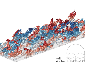Figure 4 shows iso-surfaces of $u$ in an instantaneous flow field of the APG TBL. Positive-$u$ (high speed; $u>\unicode[STIX]{x1D6FC}u_{rms}$) and negative-$u$ (low speed; $u<-\unicode[STIX]{x1D6FC}u_{rms}$) clusters are represented by red and blue, respectively, and wall-normal locations are illustrated by colour depths. The two insets show samples of the attached and detached $u$ structures. The length scales of an individual cluster are defined as the dimensions of the box circumscribing the object, i.e. $l_{x}$, $l_{y}$ and $l_{z}$ are its streamwise, wall-normal and spanwise lengths, respectively. The wall-normal height ($l_{y}$) of clusters is defined as $l_{y}=y_{max}-y_{min}$, which are the maximum and minimum distances from the wall.

Figure 4. The 3-D iso-surfaces of $u$ in the APG TBL. The left- and right-hand insets show samples of the attached and detached $u$ structures, respectively.

Figure 5. (a) Percolation diagram for the detected $u$ clusters. The variations with $\unicode[STIX]{x1D6FC}$ in the total volume ($V$) and the total number ($N$) of clusters. (b) The number of $u$ clusters per unit wall-parallel area ($n^{\ast }$) with respect to $y_{min}$ and $y_{max}$.

The percolation diagram for the identified $u$ clusters in figure 5(a) enables the choice of $\unicode[STIX]{x1D6FC}$. The percolation theory describes the statistics of the contiguous nodes in a randomly distributed system. The total number (N) and total volume ($V$) at a particular $\unicode[STIX]{x1D6FC}$ are normalized by the maximum $N$ ($N_{max}$) and $V$ ($V_{max}$) over $\unicode[STIX]{x1D6FC}$, respectively, which are the sum of the corresponding clusters for negative and positive fluctuations. The normalized volume ($V/V_{max}$) increases with decreases in $\unicode[STIX]{x1D6FC}$, and in particular it significantly changes in the range $1.2<\unicode[STIX]{x1D6FC}<1.7$, which indicates the occurrence of the percolation crisis. Within this region, the number ratio ($N/N_{max}$) shows a peak at $\unicode[STIX]{x1D6FC}=1.5$. As $\unicode[STIX]{x1D6FC}$ decreases, new clusters arise or some of the previously identified clusters become connected. The trade-off between the two effects leads to the presence of a peak in the variation in $N/N_{max}$; the former behaviour is dominant for $\unicode[STIX]{x1D6FC}>1.5$ and vice versa. In addition, the variations in $V/V_{max}$ and $N/N_{max}$ in the APG and ZPG TBLs coincide, indicating that the percolation behaviour of the $u$ clusters is independent of the pressure gradient. In the present study, we select $\unicode[STIX]{x1D6FC}=1.5$ based on the percolation transition.

Figure 5(b) shows the number of $u$ clusters per unit wall-parallel area ($A_{xz}=\unicode[STIX]{x1D6FF}_{x}\unicode[STIX]{x1D6FF}_{z}$) as a function of $y_{min}$ and $y_{max}$, which are the minimum and maximum distances from the wall:

(2.1)$$\begin{eqnarray}n^{\ast }=\frac{n(y_{min},y_{max})}{mA_{xz}},\end{eqnarray}$$

where $n$ is the number of identified $u$ clusters and $m$ is the number of instantaneous flow fields used to detect $u$ clusters ($m=2758$ for the APG TBL and 2100 for the ZPG TBL). Here, the colour and line contours of $n^{\ast }$ are for the APG and ZPG TBLs, respectively. Only the $u$ clusters with volumes larger than $30^{3}$ wall units are analysed (Del Álamo et al. Reference Del Álamo, Jiménez, Zandonade and Moser2006). The $u$ structures are divided into two groups: those are observed at $y_{min}^{+}\approx 0$ and $y_{min}^{+}>0$, i.e. the wall-attached and wall-detached structures, respectively. Following the research of Hwang & Sung (Reference Hwang and Sung2018) and Hwang & Sung (Reference Hwang and Sung2019), we defined the wall-attached objects as those with $y_{min}^{+}\approx 0$; i.e. those structures that are physically attached to the wall. Note that Townsend’s attached-eddy hypothesis does not suppose that attached eddies are physically anchored to the wall because attached eddies are assumed to be inviscid. Of course, the present study could define the attached structures as those structures with $y_{min}$ below the viscous sublayer ($y^{+}=5$) but for 80 % of such structures $y_{min}^{+}\approx 0$. In addition, 94 % of the tall structures ($l_{y}^{+}=y_{max}^{+}-y_{min}^{+}>100$ and $y_{min}^{+}<5$) examined in the present work are based on $y_{min}^{+}\approx 0$, which indicates that the results of the present study are not affected by the use of this criterion.

With the present criterion (i.e. $y_{min}^{+}\approx 0$), we can analyse the wall-normal variations of the turbulence statistics carried by these structures according to their height ($l_{y}$) without any interpolation since $l_{y}=y_{max}$. Moreover, we distinguish between the words ‘attached’ and ‘self-similar’ in contrast to several previous studies discussing the attached-eddy hypothesis because the clusters of $u$ can be decomposed into attached self-similar, attached non-self-similar, detached self-similar and detached non-self-similar motions. Here, ‘self-similar motions’ are defined as the clusters whose characteristic length scales are proportional to their height.

For the attached structures $(y_{min}^{+}\approx 0)$, $y_{max}$ varies from the near-wall region to the outer region and in particular an outer peak emerges near $y_{max}^{+}=700$, which implies the dominance of very tall attached structures in the vicinity of the boundary edge. On the other hand, the detached $u$ structures are distributed in a narrow band and are densely populated in the outer region (see § 4). A weak peak appears at $y_{min}^{+}\approx 7$ and $y_{max}^{+}\approx 50$, but its strength is at least two orders of magnitude lower than that in the outer region. The structures in this region may be associated with debris from attached structures or objects that are evolving towards attached ones (Hwang & Sung Reference Hwang and Sung2018). A further exploration of their temporal evolution is necessary, although beyond the scope of the present work.

Figure 6 shows the 3-D iso-surfaces of the intense $u$ ($|u|>1.5u_{rms}$) in the APG TBL. Through the identification of individual clusters, we can decompose $u$ fields into $u_{attached}$, $u_{detached}$ and $u_{weak}$ ($|u|<1.5u_{rms}$). The blue and red contours indicate negative $u$ and positive $u$, respectively. The intensity of the colour represents the wall-normal distance. As can be seen in this figure, the iso-surfaces of $u_{attached}$ are significantly extended in the streamwise direction, and the negative and positive $u_{attached}$ are aligned side by side along the spanwise direction. On the other hand, $u_{detached}$ is much smaller than the large $u_{attached}$.

Figure 6. The 3-D iso-surfaces of $u$ ($=u_{attached}+u_{detached}+u_{weak}$) in the APG TBL. Red and blue represent intense positive and negative $u$, respectively.

Figure 7. Profiles of (a) $\langle uu\rangle ^{+}$ and (b) $\langle uu\rangle _{attached}^{+}$ and $\langle uu\rangle _{detached}^{+}$. Profiles of (c) $\langle -uv\rangle ^{+}$ and (d) $\langle -uv\rangle _{attached}^{+}$ and $\langle -uv\rangle _{detached}^{+}$.

Next, we examine the contributions of the attached and detached $u$ structures to $\langle uu\rangle$. Figure 7(a) shows the profiles of $\langle uu\rangle ^{+}$, where the magnitude of $\langle uu\rangle ^{+}$ in the outer region is enhanced by the presence of a secondary peak near $y^{+}=240$ in the APG TBL (red line). The streamwise Reynolds stresses carried by the attached and detached $u$ structures are presented in figure 7(b) and are defined as

(2.2)$$\begin{eqnarray}\displaystyle & \displaystyle \langle u_{i}u_{j}\rangle _{attached}(y)=\frac{1}{mV_{DoI}}\iint _{\unicode[STIX]{x1D6FA}_{attached}}u_{i}(\boldsymbol{x})u_{j}(\boldsymbol{x})\,\text{d}x\,\text{d}z, & \displaystyle\end{eqnarray}$$

(2.3)$$\begin{eqnarray}\displaystyle & \displaystyle \langle u_{i}u_{j}\rangle _{detached}(y)=\frac{1}{mV_{DoI}}\iint _{\unicode[STIX]{x1D6FA}_{detached}}u_{i}(\boldsymbol{x})u_{j}(\boldsymbol{x})\,\text{d}x\,\text{d}z, & \displaystyle\end{eqnarray}$$

where $\unicode[STIX]{x1D6FA}_{attached}$ and $\unicode[STIX]{x1D6FA}_{detached}$ are the domains of all constituent points of attached and detached structures, respectively, and $V_{DoI}$ ($=\unicode[STIX]{x1D6FF}_{x}\unicode[STIX]{x1D6FF}_{y}\unicode[STIX]{x1D6FF}_{z}$) is the volume of the DoI. The attached $u$ structures account for over half of $\langle uu\rangle ^{+}$, whereas the detached $u$ structures contribute to less than 13 % of $\langle uu\rangle ^{+}$. The remainder is responsible for weak turbulence. In addition, the shape of $\langle uu\rangle _{attached}^{+}$ is similar to that of $\langle uu\rangle ^{+}$. The wall-normal location of the inner peak of $\langle uu\rangle _{attached}^{+}$ is at $y^{+}$${\approx}$ 15, and the outer peak of $\langle uu\rangle _{attached}^{+}$ arises at $y^{+}=210$. In contrast to $\langle uu\rangle _{attached}^{+}$, the profiles of $\langle uu\rangle _{detached}^{+}$ in the APG and ZPG TBLs follow each other closely up to $y^{+}=100$. At $y^{+}>100$, the magnitude of $\langle uu\rangle _{detached}^{+}$ in the APG TBL is larger than that in the ZPG TBL, and there is an outer peak at $y/\unicode[STIX]{x1D6FF}$ = 0.5. This result indicates that the detached structures within $y^{+}<100$ are defect by the pressure gradient. Note that the present Reynolds number ($Re_{\unicode[STIX]{x1D70F}}\approx 800$) is low. As the Reynolds number increases further, it is expected that the contribution of the attached structures will increase, and thus the similarity of the structures will be maintained in a manner analogous to that observed in turbulent pipe flows with $Re_{\unicode[STIX]{x1D70F}}=930$ and 3008 (Hwang & Sung Reference Hwang and Sung2019).

Figure 7(c) shows the profiles of $\langle -uv\rangle ^{+}$; a peak is located at $y^{+}=280$ in the results for the APG TBL. We compute $\langle -uv\rangle$ from the results for the attached $(\langle -uv\rangle _{attached})$ and detached $(\langle -uv\rangle _{detached})$ structures obtained from (2.2) and (2.3). The attached structures contribute over 40 % of $\langle -uv\rangle ^{+}$, which is similar to a previous result for the wall-attached ejections and sweeps of APG TBLs (Maciel et al. Reference Maciel, Gungor and Simens2017a). In the present study, the identified wall-attached structures carry approximately half of $\langle uu\rangle ^{+}$ and $\langle -uv\rangle ^{+}$, which indicates that they are the main energy-containing motions.

3.1 Self-similarity

We now examine the lengths ($l_{x}$) and widths ($l_{z}$) of the wall-attached $u$ structures to determine whether the sizes of the type A and type B structures can be characterized with $l_{y}$ and $\unicode[STIX]{x1D6FF}$, respectively. Figure 9 shows the joint PDFs of $l_{x}$ and $l_{z}$ of the wall-attached $u$ structures with respect to $l_{y}$. Here, the contours and lines indicate the distributions for the APG and ZPG TBLs, respectively. The mean $l_{x}$ and $l_{z}$ at a given $l_{y}$ are shown as circles: APG (red) and ZPG (black). In figure 9(a), the mean $l_{x}$ of the type A structures ($100<l_{y}^{+}<0.6\unicode[STIX]{x1D6FF}^{+}$) scales with $l_{y}$, following the power law $l_{x}\sim l_{y}^{0.74}$ (yellow solid line). Above $l_{y}^{+}>0.6\unicode[STIX]{x1D6FF}^{+}$, the mean $l_{x}$ rapidly increases and exhibits a constant value $l_{x}^{+}\approx 3.5\unicode[STIX]{x1D6FF}^{+}$ for $l_{y}^{+}>\unicode[STIX]{x1D6FF}^{+}$ (blue horizontal line), which indicates that very tall structures (i.e. type B) are non-self-similar ($O(3\unicode[STIX]{x1D6FF}{-}6\unicode[STIX]{x1D6FF})$). In addition, there are protrusions in the contours near $l_{y}^{+}\approx \unicode[STIX]{x1D6FF}^{+}$, i.e. superstructures or VLSMs. In figure 9(b), a linear relationship is evident between the mean $l_{z}$ and $l_{y}$ (yellow solid line) from $l_{y}^{+}=100$ to $l_{y}^{+}=\unicode[STIX]{x1D6FF}^{+}$. In other words, the spanwise length of attached $u$ structures ($l_{y}^{+}>100$) is proportional to the distance from the wall (Tomkins & Adrian Reference Tomkins and Adrian2003; Del Álamo et al. Reference Del Álamo, Jiménez, Zandonade and Moser2006; Sillero Reference Sillero2014; Hwang Reference Hwang2015; Hwang & Sung Reference Hwang and Sung2018, Reference Hwang and Sung2019). In particular, the width distributions for the APG and ZPG TBLs collapse well, reflecting that the spanwise length scales of the attached $u$ structures are not significantly affected by the APG. In sum, type A structures are geometrically self-similar with respect to $l_{y}$, whereas the streamwise length of type B motions scales with the outer length scale.

Figure 9. Joint PDFs of (a) $l_{x}$ and $l_{y}$ and of (b) $l_{z}$ and $l_{y}$. Circles indicate mean lengths. The yellow line in (a) represents $l_{x}^{+}\sim (l_{y}^{+})^{0.74}$ and in (b) $l_{z}^{+}=l_{y}^{+}$.

3.2 Reynolds stresses

The streamwise Reynolds stresses and the Reynolds shear stresses carried by type A and type B structures are defined as

(3.2)$$\begin{eqnarray}\displaystyle & \displaystyle \langle u_{i}u_{j}\rangle _{A}(y)=\frac{1}{mV_{DoI}}\mathop{\sum }_{l_{y}^{+}=100}^{l_{y}/\unicode[STIX]{x1D6FF}=0.6}\iint _{\unicode[STIX]{x1D6FA}_{attached}(l_{y})}u_{i}(\boldsymbol{x})u_{j}(\boldsymbol{x})\,\text{d}x\,\text{d}z, & \displaystyle\end{eqnarray}$$

(3.3)$$\begin{eqnarray}\displaystyle & \displaystyle \langle u_{i}u_{j}\rangle _{B}(y)=\frac{1}{mV_{DoI}}\mathop{\sum }_{l_{y}/\unicode[STIX]{x1D6FF}=0.6}^{l_{y}=\unicode[STIX]{x1D6FF}_{y}}\iint _{\unicode[STIX]{x1D6FA}_{attached}(l_{y})}u_{i}(\boldsymbol{x})u_{j}(\boldsymbol{x})\,\text{d}x\,\text{d}z. & \displaystyle\end{eqnarray}$$

Hereafter, subscripts $A$ and $B$ denote averaged quantities of type A and type B structures, respectively. Here, $\unicode[STIX]{x1D6FF}_{y}$ ($=1.7\unicode[STIX]{x1D6FF}$) is the wall-normal size of the DoI. Figure 10(a) shows the wall-normal profiles of $\langle uu\rangle _{A}^{+}$ for the APG (red) and ZPG (black) TBLs. Interestingly, both profiles follow the logarithmic profile in the region $y^{+}=100{-}0.3\unicode[STIX]{x1D6FF}^{+}$. The attached self-similar structures ($100<l_{y}^{+}<0.6\unicode[STIX]{x1D6FF}^{+}$) show the statistical features of type A eddies (Perry & Marusic Reference Perry and Marusic1995). In other words, these structures exhibit universal motion and directly contribute to the presence of the logarithmic region. In contrast, $\langle uu\rangle _{B}^{+}$ for the APG TBL is entirely different from that for the ZPG TBL with a distinct outer peak at $y^{+}=230$ (figure 10b). The enhanced streamwise Reynolds stress carried by the attached $u$ structures ($\langle uu\rangle _{attached}^{+}$, shown in figure 7b) in the APG TBL is due to the contribution of the type B structures ($l_{y}/\unicode[STIX]{x1D6FF}>0.6$). The magnitude of the outer peak ($y^{+}\approx 240$) is greater than that of the inner peak at $y^{+}\approx 15$, which reflects the fact that the attached $u$ structures with $l_{y}/\unicode[STIX]{x1D6FF}>0.6$ are responsible for the wake region. Moreover, there is no logarithmic variation in $\langle uu\rangle _{B}^{+}$. Given that the logarithmic variation in the streamwise Reynolds stress is contaminated by very long and wide motions (Jiménez & Hoyas Reference Jiménez and Hoyas2008), the absence of logarithmic variation in figure 10(b) indicates that the tall attached $u$ structures are associated with VLSMs or superstructures. In figure 10(c,d), the profiles of $\langle -uv\rangle _{A}^{+}$ and $\langle -uv\rangle _{B}^{+}$ exhibit behaviours similar to those observed in the streamwise Reynolds stress. The profiles of $\langle -uv\rangle _{A}^{+}$ are similar to each other across the wall-normal locations, whereas $\langle -uv\rangle _{B}^{+}$ for the APG TBL increases significantly and contains a strong outer peak.

Figure 10. Profiles of (a) $\langle uu\rangle _{A}^{+}$ and (b) $\langle uu\rangle _{B}^{+}$. Profiles of (c) $\langle -uv\rangle _{A}^{+}$ and $\langle -uv\rangle _{B}^{+}$. The blue lines indicate logarithmic variation in $\langle uu\rangle _{i}^{+}$: $\langle uu\rangle _{A}^{+}=-0.37\ln (y^{+})+2.12$ over the range $y^{+}=100{-}0.3\unicode[STIX]{x1D6FF}^{+}$ for the APG TBL and $\langle uu\rangle _{A}^{+}=-0.32\ln (y^{+})+1.84$ over the range $y^{+}=100{-}0.3\unicode[STIX]{x1D6FF}^{+}$ for the ZPG TBL. The vertical lines in (a) represent $y^{+}=100$ and $0.3\unicode[STIX]{x1D6FF}^{+}$.

Figure 11. Spectra (a) $k_{z}\unicode[STIX]{x1D719}_{uu,A}^{+}$ and (b) $k_{z}\unicode[STIX]{x1D719}_{uu,B}^{+}$. The colour and line contours are for the APG and ZPG TBLs, respectively. The line contour level is equivalent to the colour contour level. In (a), vertical lines represent $y^{+}=160$ and 205, and the yellow dashed line is $\unicode[STIX]{x1D706}_{z}=5y$.

3.3 Spanwise spectra

To further examine the streamwise Reynolds stress carried by type A and type B structures, figure 11 shows their pre-multiplied spanwise energy spectra based on conditional velocity fields:

(3.4)$$\begin{eqnarray}\displaystyle & \displaystyle u_{A}(\boldsymbol{x},t)=\left\{\begin{array}{@{}l@{}}u,\quad \text{if }|u|>1.5u_{rms},y_{min}^{+}\approx 0\text{ and }100<l_{y}^{+}<0.6\unicode[STIX]{x1D6FF}^{+},\\ 0,\quad \text{otherwise},\end{array}\right. & \displaystyle\end{eqnarray}$$

(3.5)$$\begin{eqnarray}\displaystyle & \displaystyle u_{B}(\boldsymbol{x},t)=\left\{\begin{array}{@{}l@{}}u,\quad \text{if }|u|>1.5u_{rms},y_{min}^{+}\approx 0\text{ and }l_{y}/\unicode[STIX]{x1D6FF}>0.6,\\ 0,\quad \text{otherwise}.\end{array}\right. & \displaystyle\end{eqnarray}$$

The spanwise spectra $\unicode[STIX]{x1D719}_{uu,A}$ and $\unicode[STIX]{x1D719}_{uu,B}$ are obtained from the Fourier transform of $u_{A}$ and $u_{B}$, respectively:

(3.6)$$\begin{eqnarray}\unicode[STIX]{x1D719}_{uu,i}(k_{z},y)=\frac{1}{\unicode[STIX]{x1D6FF}_{x}}\int _{-\infty }^{\infty }\text{Re}\{F\hat{F}\}\,\text{d}(x/\unicode[STIX]{x1D6FF}),\end{eqnarray}$$

where $F$ is the Fourier coefficient of $u_{i}(\boldsymbol{x},t)$, Re is the real part of a complex and the caret denotes a complex conjugate. The profiles of $\langle uu\rangle _{A}$ and $\langle uu\rangle _{B}$ in figure 10(a,b) can be obtained from the integration of pre-multiplied spectra with respect to $\ln k_{z}$: $\langle uu\rangle _{A}(y)=\int _{-\infty }^{\infty }k_{z}\unicode[STIX]{x1D719}_{uu,A}(k_{z},y)\,\text{d}\ln k_{z}$ and $\langle uu\rangle _{B}(y)=\int _{-\infty }^{\infty }k_{z}\unicode[STIX]{x1D719}_{uu,B}(k_{z},y)\,\text{d}\ln k_{z}$, respectively. The spectrum $k_{z}\unicode[STIX]{x1D719}_{uu,\,A}(k_{z},y)$ is the distribution of the streamwise Reynolds stress among various spanwise wavelengths contained by type A structures with $y<l_{y}$. Note that an individual attached $u$ structure with size $l_{y}$ contains shorter objects with heights less than $l_{y}$ (i.e. nested hierarchies), because the attached $u$ structures consist of multiple uniform momentum zones and the streamwise Reynolds stress of the attached structures increases with $l_{y}$ along the wall-normal direction (see § 5 in Hwang & Sung (Reference Hwang and Sung2018)). In addition, although the attached-eddy models assume statistically representative structures that possess the gross features of an assemblage of eddies (Perry & Marusic Reference Perry and Marusic1995), we expect an individual $u$ structure to contain spanwise wavelengths in the range $\unicode[STIX]{x1D706}_{z}\leqslant l_{z}$ (${\approx}l_{y}$; figure 9b), not a single $\unicode[STIX]{x1D706}_{z}$ for a given $l_{y}$ (Nickels et al. Reference Nickels, Marusic, Hafez, Hutchins and Chong2007). In this sense, if these types of structures satisfy the spectral signature of the attached-eddy hypothesis, then $k_{z}\unicode[STIX]{x1D719}_{uu,A}^{+}$ contains a $k_{z}^{-1}$ region without peaks in the low-wavenumber range, whereas $k_{z}\unicode[STIX]{x1D719}_{uu,B}^{+}$ contains a dominant peak at large scales but no $k_{z}^{-1}$ region.

Figure 11(a) shows $k_{z}\unicode[STIX]{x1D719}_{uu,A}^{+}$ for the APG (colour contour) and ZPG (line contour) TBLs. As this figure shows, the contours of $k_{z}\unicode[STIX]{x1D719}_{uu,A}^{+}$ coincide despite the presence of the APG. In the near-wall region, $k_{z}\unicode[STIX]{x1D719}_{uu,A}^{+}$ has an inner peak at $\unicode[STIX]{x1D706}_{z}^{+}=92$ due to near-wall streaks (Kline et al. Reference Kline, Reynolds, Schraub and Runstadler1967). Since the attached $u$ structures are in the form of nested hierarchies, they include small scales in the near-wall region, which results in the inner peak at $y^{+}=18$. The spectra $k_{z}\unicode[STIX]{x1D719}_{uu,A}^{+}$ are aligned along a linear ridge ($\unicode[STIX]{x1D706}_{z}=5y$), representing that the spanwise length scale of type A is proportional to the distance from the wall in spectral space (Hoyas & Jiménez Reference Hoyas and Jiménez2006; Hwang Reference Hwang2015; Chandran et al. Reference Chandran, Baidya, Monty and Marusic2017). Two peaks are evident in both contour maps in figure 11(b), but $k_{z}\unicode[STIX]{x1D719}_{uu,B}^{+}$ in the presence of the APG is nevertheless distinctly different from that of the ZPG case. The outer peak is remarkably intense at $\unicode[STIX]{x1D706}_{z}^{+}=640$ ($\unicode[STIX]{x1D706}_{z}/\unicode[STIX]{x1D6FF}=0.83$) and $y^{+}=230$ ($y/\unicode[STIX]{x1D6FF}=0.3$). Here, the large and small scales are split according to a cutoff spanwise wavelength of $\unicode[STIX]{x1D706}_{z},_{c}^{+}=400$ ($\unicode[STIX]{x1D706}_{z},_{c}/\unicode[STIX]{x1D6FF}\approx 0.5$) (Bernardini & Pirozzoli Reference Bernardini and Pirozzoli2011; Hwang & Sung Reference Hwang and Sung2017; Yoon et al. Reference Yoon, Hwang and Sung2018). The footprints of the large-scale energy in the outer region of $k_{z}\unicode[STIX]{x1D719}_{uu,B}^{+}$ penetrate into the near-wall region (Hutchins & Marusic Reference Hutchins and Marusic2007a), and outer large scales modulate the amplitudes of small scales (Bernardini & Pirozzoli Reference Bernardini and Pirozzoli2011).

Figure 12(a) shows the profiles of $k_{z}\unicode[STIX]{x1D719}_{uu,A}^{+}/\langle uu\rangle _{A}^{+}$ with respect to $\unicode[STIX]{x1D706}_{z}^{+}/y^{+}$ at four wall-normal locations ($y^{+}=160$, 175, 190 and 205), which are chosen in the vicinity of the centre of the logarithmic region of $\langle uu\rangle _{A}^{+}$ (figure 10a). The profiles collapse in the region $\unicode[STIX]{x1D706}_{z}^{+}/y^{+}=1.2{-}2.0$, where $k_{z}\unicode[STIX]{x1D719}_{uu,A}^{+}/\langle uu\rangle _{A}^{+}$ is constant. As for the outer scaling ($\unicode[STIX]{x1D706}_{z}/\unicode[STIX]{x1D6FF}$), the profiles in figure 12(b) collapse in a single curve in the region $\unicode[STIX]{x1D706}_{z}/\unicode[STIX]{x1D6FF}=0.28{-}0.45$. The $k_{z}^{-1}$ region (a plateau) is observed in $k_{z}\unicode[STIX]{x1D719}_{uu,A}^{+}/\langle uu\rangle _{A}^{+}$ in the region $\unicode[STIX]{x1D706}_{z}^{+}/y^{+}>1.2$ and $\unicode[STIX]{x1D706}_{z}/\unicode[STIX]{x1D6FF}<0.45$, where both the inner scaling and outer scaling are simultaneously valid (Perry & Abell Reference Perry and Abell1977; Perry et al. Reference Perry, Henbest and Chong1986; Nickels et al. Reference Nickels, Marusic, Hafez and Chong2005). Note that the $k_{x}^{-1}$ or $k_{z}^{-1}$ regions do not indicate the spectra collapse over all the range of wavelength. For example, the lower and upper limits of the $k_{x}^{-1}$ region are $\unicode[STIX]{x1D706}_{x}/y>15.7$ and $\unicode[STIX]{x1D706}_{x}/\unicode[STIX]{x1D6FF}<0.3$ (Nickels et al. Reference Nickels, Marusic, Hafez and Chong2005) and $\unicode[STIX]{x1D706}_{x}/y>12$ and $\unicode[STIX]{x1D706}_{x}/\unicode[STIX]{x1D6FF}<2$ (Hwang Reference Hwang2015). Here, $\unicode[STIX]{x1D706}_{x}$ ($=2\unicode[STIX]{x03C0}/k_{x}$) is the streamwise wavelength. Given the self-similarity ($\unicode[STIX]{x1D706}_{x}\sim 10\unicode[STIX]{x1D706}_{z}$) of the main energy-containing motions in Hwang (Reference Hwang2015), the present $k_{z}^{-1}$ region in $k_{z}\unicode[STIX]{x1D719}_{uu,A}^{+}/\langle uu\rangle _{A}^{+}$ is in good agreement with previous results. The profiles of $k_{z}\unicode[STIX]{x1D719}_{uu,A}^{+}/\langle uu\rangle _{A}^{+}$ exhibit the $k_{z}^{-1}$ region, leading to the logarithmic variation in $\langle uu\rangle _{A}^{+}$. Baars & Marusic (Reference Baars and Marusic2020b) reported that the logarithmic slope of $\langle uu\rangle ^{+}$ reconstructed from type A energy decreases logarithmically with respect to $y^{+}$ at lower Reynolds numbers ($Re_{\unicode[STIX]{x1D70F}}=O(10^{3})$) but is constant over a certain region at higher Reynolds numbers ($Re_{\unicode[STIX]{x1D70F}}>O(10^{4})$). There is a $k_{z}^{-1}$ region in $k_{z}\unicode[STIX]{x1D719}_{uu,A}^{+}/\langle uu\rangle _{A}^{+}$, which confirms that attached eddies are responsible for the plateau region in the pre-multiplied spectra scaled by both the inner scaling $y$ and outer scaling $\unicode[STIX]{x1D6FF}$ (Perry et al. Reference Perry, Henbest and Chong1986).

Figure 12(c) shows the profiles of $k_{z}\unicode[STIX]{x1D719}_{uu,B}^{+}/\langle uu\rangle _{B}^{+}$ at $y/\unicode[STIX]{x1D6FF}=0.3$, 0.4 and 0.5 as a function of $(\unicode[STIX]{x1D706}_{z}/\unicode[STIX]{x1D6FF})/(y/\unicode[STIX]{x1D6FF})$. As can be seen in this figure, the profiles do not coincide, but the magnitude of the peaks is 0.45 regardless of the pressure gradient. Interestingly, those profiles collapse into a single curve with respect to $\unicode[STIX]{x1D706}_{z}/\unicode[STIX]{x1D6FF}$ (figure 12d), which indicates that outer scaling is suitable for type B structures. The peaks converge at $\unicode[STIX]{x1D706}_{z}/\unicode[STIX]{x1D6FF}=0.8$, for which the spanwise wavelength motions in type B are the dominant contributors to $\langle uu\rangle _{B}^{+}$ in the outer region, and thus there is an outer peak in $\langle uu\rangle _{B}^{+}$. In addition, that is equivalent to $\unicode[STIX]{x1D706}_{z}$ at the outer peak in $k_{z}\unicode[STIX]{x1D719}_{uu}^{+}$ in the APG TBLs with similar $\unicode[STIX]{x1D6FD}$ (Kitsios et al. Reference Kitsios, Sekimoto, Atkinson, Sillero, Borrell, Gungor, Jiménez and Soria2017; Lee Reference Lee2017; Yoon et al. Reference Yoon, Hwang and Sung2018), which indicates that type B structures play an important role in the outer region.

Figure 12. Profiles of $k_{z}\unicode[STIX]{x1D719}_{uu,A}^{+}/\langle uu\rangle _{A}^{+}$ with respect to (a) $\unicode[STIX]{x1D706}_{z}^{+}/y^{+}$ and (b) $\unicode[STIX]{x1D706}_{z}/\unicode[STIX]{x1D6FF}$ at $y^{+}=160$, 175, 190 and 205, and those of $k_{z}\unicode[STIX]{x1D719}_{uu,B}^{+}/\langle uu\rangle _{B}^{+}$ as functions of (c) $(\unicode[STIX]{x1D706}_{z}/\unicode[STIX]{x1D6FF})/(y/\unicode[STIX]{x1D6FF})$ and (d) $\unicode[STIX]{x1D706}_{z}/\unicode[STIX]{x1D6FF}$ at $y/\unicode[STIX]{x1D6FF}=0.3$, 0.4 and 0.5.

Next, we examine the pre-multiplied spanwise co-spectra of $\langle -uv\rangle$ carried by type A and type B structures, which can be obtained from (3.4)–(3.6). The spectrum $k_{z}\unicode[STIX]{x1D719}_{-uv,A}^{+}$ has an inner peak at $\unicode[STIX]{x1D706}_{z}^{+}=100$ and $y^{+}=54$, and similar results are obtained for the ZPG TBL (figure 13a). The large scales in the outer region are the main contributors to $k_{z}\unicode[STIX]{x1D719}_{-uv,B}^{+}$ as shown by the outer peak at $\unicode[STIX]{x1D706}_{z}^{+}=640$ ($\unicode[STIX]{x1D706}_{z}/\unicode[STIX]{x1D6FF}=0.83$) and $y^{+}=270$ ($y/\unicode[STIX]{x1D6FF}=0.35$), which results in an outer peak in the production of turbulent kinetic energy for the APG TBL (Skåre & Krogstad Reference Skåre and Krogstad1994; Lee & Sung Reference Lee and Sung2008; Kitsios et al. Reference Kitsios, Atkinson, Sillero, Borrell, Gungor, Jiménez and Soria2016, Reference Kitsios, Sekimoto, Atkinson, Sillero, Borrell, Gungor, Jiménez and Soria2017) and thus in an increase in large-scale activity in the outer region. As shown in figure 11(b), the long-wavelength energy of $k_{z}\unicode[STIX]{x1D719}_{uu,B}^{+}$ in the outer region penetrates into the near-wall region, whereas that of $k_{z}\unicode[STIX]{x1D719}_{-uv,B}^{+}$ diminishes near the wall (figure 13b) due to an impermeable wall. This behaviour is equivalent to that reported previously (Jiménez & Hoyas Reference Jiménez and Hoyas2008; Hwang Reference Hwang2015). Hwang (Reference Hwang2015) argued that these inactive motions are the near-wall parts of VLSMs (i.e. the footprint) that contribute negligibly to the Reynolds shear stress in the near-wall region compared to their contributions in the logarithmic region. In other words, the active or inactive characteristics of very large motions depend on their wall-normal locations (Nickels et al. Reference Nickels, Marusic, Hafez, Hutchins and Chong2007).

Figure 13. Spectra (a) $k_{z}\unicode[STIX]{x1D719}_{-uv,A}^{+}$ and (b) $k_{z}\unicode[STIX]{x1D719}_{-uv,B}^{+}$ for the APG and ZPG TBLs.