


1 Introduction
1.1 Motivation
A porous body impinged by a turbulent boundary layer is a flow phenomenon that is widely encountered in environmental and industrial fluid mechanics. Examples include atmospheric boundary layers over patches of forest, wind farms or buildings, rivers over vegetated beds, currents impinging on offshore structures and tidal turbines, to name just a few. In all these examples the porous body can be represented as an array of obstacles, which modifies the flow affecting momentum, energy and scalar transport processes, which are economically and environmentally relevant.
From an environmental perspective, arrays made of aquatic and terrestrial vegetation play an important role on the functioning of aquatic and terrestrial ecosystems. As a matter of fact, flow resistance exerted by vegetation provides sheltering and habitat for aquatic fauna (Kemp, Harper & Crosa Reference Kemp, Harper and Crosa2000) in rivers; the multiple length scales characterizing the arrays, ranging from the array size to the size of its constitutive components, dictate multiscale flow structures, which in turn affect sediment deposition and erosion patterns (De Langre Reference De Langre2008; Nepf Reference Nepf2012) and scalar (i.e. oxygen, nutrients, pollen) exchange with the surrounding fluid (Poggi, Katul & Albertson Reference Poggi, Katul and Albertson2006).
In urban meteorology, the landscape topology has been proven to play an analogous role in promoting multiscale coherent structures altering the momentum exchange (Vanderwel & Tavoularis Reference Vanderwel and Tavoularis2015) and the quality of the air, impacting the transport of heat and chemical species.
From an industrial point of view, the load applied on the array is of primary importance to forecast the energy harvested in classic (e.g. tidal and wind farms; see Vennell (Reference Vennell2011) and Myers & Bahaj (Reference Myers and Bahaj2012)) and innovative systems (e.g. piezoelectric grass extracting energy from fluid flows; see Hobeck & Inman (Reference Hobeck and Inman2012)) as well as for the structural design of the individual components of the array, to avoid damage and fatigue degradation (Gardiner, Peltola & Kellomäki Reference Gardiner, Peltola and Kellomäki2000). The energy production from groups of turbines comes at the cost of the impact that the wake of the farms and of each individual turbine produce on its surrounding areas. In the case of wind turbines, alterations in the local meteorology will affect the vertical distribution of heat and humidity (Baidya Roy, Pacala & Walko Reference Baidya Roy, Pacala and Walko2004; Rajewski et al. Reference Rajewski, Takle, Prueger and Doorenbos2016), which can affect, for example, the productivity of agricultural sites. Farms installed in oceans and rivers represent the frontier for renewable energy production, but the array configuration and density have been proven to alter not only the output energy but also the installation site (Ahmadian, Falconer & Bockelmann-Evans Reference Ahmadian, Falconer and Bockelmann-Evans2012). For example, tidal farms are known to reduce tidal currents up to 15 % and this has consequences on sediment dynamics, bacterial life cycle and fish migration.
1.2 Literature
From a modelling point of view, all the mentioned interactions have been so far schematized and studied mostly as canonical canopy flows, i.e. turbulent boundary layers growing over uniformly distributed roughness elements composing the canopy. Although this approach has led to the identification of distinctive features characterizing the near-wall turbulence structure (Raupach, Finnigan & Brunet Reference Raupach, Finnigan and Brunet1996; Ghisalberti & Nepf Reference Ghisalberti and Nepf2002), its applicability, in environmental and industrial contexts, is strongly limited by the fact that canonical canopy flows are rarely encountered. As a matter of fact, canopies are rather distributed in patches whose free ends play a crucial role in dictating the dynamics of the interaction with the surrounding flow.
The increasing attention towards the understanding of the mechanisms triggered by such patches is testified by the recent increase in the investigations addressing this topic (Nicolle & Eames Reference Nicolle and Eames2011; Chen et al. Reference Chen, Ortiz, Zong and Nepf2012; Zong & Nepf Reference Zong and Nepf2012; Chang & Constantinescu Reference Chang and Constantinescu2015; Chang, Constantinescu & Tsai Reference Chang, Constantinescu and Tsai2017). All of them explore the case of a turbulent flow impinging on a group of cylinders whose height covers the entire vertical length of the flow domain. This is meant to model, e.g. the flow past emergent vegetation or a group of tall offshore risers that pierce the free surface of the ocean. At these conditions, the mean flow can be considered, to a good approximation, as two-dimensional and it was observed to be dependent on the following dimensional parameters: the number of cylinders within the patch  $N_{c}$, the diameter of the cylinders constituting the patch
  $d$ and, in case the patch has a circular section, its diameter
  $D$. Such parameters can be combined to form non-dimensional groups that describe and explain some characteristic features of flows interacting with canopy patches and, in general, with porous obstacles. Much of the most recent literature highlights that the patch density (
 $\unicode[STIX]{x1D719}$), defined as the planar area covered by cylinders per total surface (also often referred to as the solid volume fraction), i.e.
  $\unicode[STIX]{x1D719}=N_{c}(d/D)^{2}$ is the key parameter to describe the wake past canopy patches. Nicolle & Eames (Reference Nicolle and Eames2011) carried out two-dimensional direct numerical simulations (DNS), fixing the ratio
  $d/D$ and exploring the flow around patches having a wide range of
  $N_{c}$. Their results helped to identify three different wake structures based on
  $\unicode[STIX]{x1D719}$: a low density regime, for
  $\unicode[STIX]{x1D719}<0.05$, where individual non-interacting wakes form end evolve downwind of the patch; an intermedium density regime, for
  $0.05<\unicode[STIX]{x1D719}<0.15$, where the constitutive cylinders are close enough for individual wakes to merge giving origin to a single wake; a high density regime (
 $\unicode[STIX]{x1D719}>0.15$), where most of the flow is diverted around the patch, which acts almost as a solid body. Nicolle & Eames (Reference Nicolle and Eames2011), Zong & Nepf (Reference Zong and Nepf2012) and Taddei, Manes & Ganapathisubramani (Reference Taddei, Manes and Ganapathisubramani2016) report the presence of a so-called steady-wake region, namely, a flow region of the wake, located in proximity to the trailing edge of the patch, where the longitudinal velocity is approximately constant. The presence of this zone is a prerogative of porous bodies, as a consequence of the fraction of flow penetrating the body. Zong & Nepf (Reference Zong and Nepf2012) report that, for the range of assessed patch diameters and densities, the steady velocity normalized with the impinging flow velocity
  $U_{\infty }$,
  $U_{1}/U_{\infty }$ and the non-dimensional longitudinal extent of the steady-wake region,
  $L_{1}/D$ scaled nicely with
  $\unicode[STIX]{x1D719}$. In interpreting the results associated with
  $U_{1}$ and building upon the work by Rominger & Nepf (Reference Rominger and Nepf2011), Zong & Nepf (Reference Zong and Nepf2012) classify porous patches on the basis of the parameter
  $C_{d}aD$, where
  $C_{d}$ is the mean drag coefficient of a cylinder within the patch (often approximated as that of an infinite isolated cylinder at high Reynolds number:
  $C_{d}=1$) and
  $a$ is the frontal area per unit volume defined as
  $a=N_{c}d/(0.25\unicode[STIX]{x03C0}D^{2})$. The parameter
  $C_{d}aD$ is crucial in quantifying the so-called interior adjustment length scale
  $x_{d}$, which is the length required by the flow within an indefinitely long patch (i.e. a patch of length much larger than width) to adjust to a steady value after impingement at the lee side. For
  $C_{d}aD\ll 4$, patches are classified as low-flow blockage and
  $x_{d}$ is larger than the diameter
  $D$ of the patch. For
  $C_{d}aD\gg 4$, the patches are classified as high-flow blockage and
  $x_{d}$ is lower than
  $D$. Interestingly, for
  $C_{d}aD\gg 4$, Zong & Nepf (Reference Zong and Nepf2012) observed that
  $U_{1}$ coincided with the interior velocity
  $U_{0}$ predicted for an infinite patch by Rominger & Nepf (Reference Rominger and Nepf2011). Conversely, for
  $C_{d}aD\ll 4$,
  $U_{1}$ was observed to be always higher than
  $U_{0}$.
While most of the wake properties can be nicely captured by  $\unicode[STIX]{x1D719}$ only, drag forces and drag coefficients of the entire patch were observed by Chang & Constantinescu (Reference Chang and Constantinescu2015) to be a function of
  $\unicode[STIX]{x1D719}$ and
  $d/D$. In particular, these authors report that for
  $\unicode[STIX]{x1D719}=0.2$, doubling
  $d/D$ results in a significant change in the
  $C_{D}$ of the patch.
Although the aforementioned studies have greatly advanced the current knowledge on the drag and wakes of obstacle arrays, in many relevant applications, such arrays are fully immersed within a deep turbulent boundary layer. This leads to the formation of a mixing layer at the top of the array, which presumably interacts with the shear layers originating at the sides to generate a three-dimensional wake whose properties have not been investigated in depth yet. Moreover, this three-dimensional (3-D) configuration introduces two further relevant length scales: the vertical extent of the flow,  $h$, and the canopy vertical extent,
  $H$. A continuous and homogeneous canopy, whose height is lower than the height of the flow, is usually referred to as a submerged canopy. The specific submergence ratio,
  $h/H$, is indicative of the relative importance of the forces dominating the patch–flow interaction: the turbulent stress produced by the shear layer developing at the top of the canopy and the streamwise pressure gradients. A canopy is deeply submerged if
  $h/H>10$, while, for
  $h/H<5$, it is classified as shallow submerged (Nepf Reference Nepf2012).

Figure 1. (a) Trailing edge and lateral bleeding formation. (b) Vertical bleeding formation.
So far, the paper by Taddei et al. (Reference Taddei, Manes and Ganapathisubramani2016) represents the first study where the case of a circular patch of canopy in a submerged configuration and under the action of a turbulent boundary layer was investigated. This study highlighted how the interaction between top and lateral mixing layers strongly impacted the magnitude of the drag forces and the wake characteristics. The experiments in Taddei et al. (Reference Taddei, Manes and Ganapathisubramani2016) were carried out with a submergence ratio  $h/H>1$, while retaining the same patch planar configuration used by Nicolle & Eames (Reference Nicolle and Eames2011). In particular, Taddei et al. (Reference Taddei, Manes and Ganapathisubramani2016) report how the drag coefficient of different arrays is dictated by so-called bleeding effects, where bleeding is intended as the fluid flow through and perpendicular to the sides (lateral bleeding), the rear (trailing edge bleeding) and the top (vertical bleeding) surface of the array (figure 1). This is intuitive, because bleeding patterns are the consequence of the macroscopic pressure distribution around the surface of the patch (and the permeability of the patch itself, which allows for interstitial flow to develop) and therefore of the total drag force exerted by the fluid on the patch. In particular, in Taddei et al. (Reference Taddei, Manes and Ganapathisubramani2016), on increasing the patch density, the vertical bleeding was observed to increase whereas the trailing edge bleeding was observed to decrease. Within the limited range of the investigated densities, the drag coefficient
  $C_{D}$ was observed to increase with increasing patch density, with a levelling off for the higher densities (
 $\unicode[STIX]{x1D719}>0.15$). While no explanation was given for the levelling off, the general increasing trend of
  $C_{D}$ was explained as follows: the decrease in trailing edge bleeding promotes an increase in momentum deficit while the increase in vertical bleeding counteracts turbulent entrainment, hence preventing wake recovery. Both effects contribute to an increase of the patch’s drag coefficient. These results (including the drag levelling off for dense patches) are confirmed by the recent work by Zhou & Venayagamoorthy (Reference Zhou and Venayagamoorthy2019), which numerically explores the flow behaviour within and around an array of cylinders on changing array density and bulk aspect ratio, the latter defined as the ratio of patch height to diameter (
 $H/D$). In this case, the array is suspended in deep water and exposed to a uniform impinging flow. They conclude that the role played by the bulk aspect ratio in setting the bleeding velocity is analogous to the one played by
  $\unicode[STIX]{x1D719}$: at increasing
  $H/D$, the streamwise bleeding velocity decreases, while the vertical and lateral ones are found to increase.
Although the study by Taddei et al. (Reference Taddei, Manes and Ganapathisubramani2016) identifies and explains the link between the drag and bleeding effects, the wake topology as well as its recovery were not explored. The goal of the present work is, therefore, to complement the above mentioned study, reconsidering in further detail the available velocity measurements, so as to provide a quantitative analysis for the recovery of the velocity deficit at different array densities. The paper is organized as follows. Section 2 briefly summarizes the experimental methodology as reported in Taddei et al. (Reference Taddei, Manes and Ganapathisubramani2016); § 3 presents the analysis of the main experimental results together with empirical laws modelling the wake behaviour; § 4 is devoted to conclusions.
Table 1. (a) Main impinging flow parameters evaluated with hot-wire anemometry at  $x=0$: turbulent boundary layer thickness at 99 % of the free-stream velocity, friction velocity, equivalent roughness length, displacement thickness, momentum thickness and Reynolds number. (b) Body geometrical parameters:
  $N_{c}$ is the cylinder number in the porous body,
  $\unicode[STIX]{x1D719}$ is the corresponding density. In addition, the body height and overall diameter are
  $H=D=100$ mm and the inner cylinder diameter is
  $d=0.05D$. Here
  $aD$ is the non-dimensional frontal area per unit volume.

2 Methodology
The experiments were carried out in a suction wind tunnel at the University of Southampton, whose test section is  $0.9~\text{m}\times 0.6~\text{m}\times 4.5~\text{m}$. Beside the benchmark case, represented by a solid cylinder with height (
 $H$) and diameter (
 $D$) equal to 100 mm, five patches, of the same height (
 $H$) and diameter (
 $D$), with different densities (
 $\unicode[STIX]{x1D719}$), were also investigated; the main geometrical characteristics are listed in table 1 bottom. Each patch was placed at the centre of the test section and velocity measurements were carried out by means of particle image velocimetry (PIV) downwind of the patch. Figure 2 provides a schematic view of the measurement domain and of the coordinate system, which is used throughout the paper. The arrangement of the cylinders forming the patch was set to follow an evenly spaced distribution on concentric evenly spaced circles plus an extra cylinder at the centre of the patch: the distance between two cylinders, on each circle in the patch, was constant and equal to the distance between two consecutive circles in the patch, as proposed by Nicolle & Eames (Reference Nicolle and Eames2011). Following this rule and increasing the total number of cylinders covering the surface, the investigated densities were
  $\unicode[STIX]{x1D719}=(0.0175,0.0500,0.0975,0.1600,0.2375,1)$.

Figure 2. Schematic of the experiment and coordinate system: the coloured planes represent the field of view of the planar PIV studies.
It should be pointed out that the present experiments were carried out by varying  $\unicode[STIX]{x1D719}$ while keeping
  $d/D$ constant. In doing so, the non-dimensional frontal area per unit volume
  $aD$ (which is important to classify patches as low- or high-flow blockage as per Zong & Nepf (Reference Zong and Nepf2012)) varied from one experiment to the other (see table 1 bottom). The tested models will be referred to as
  $C7$,
$C7$,  $C20$,
  $C39$,
  $C64$,
  $C95$ according to the number of cylinders forming the array, while
  $CS$ will refer to the solid case.

Figure 3. (a) Mean velocity profile of the incoming boundary layer (symbols):  $u_{bl}$ is the time-averaged velocity,
  $D$ is the patch diameter,
  $U_{\infty }$ is the free-stream velocity,
  $y$ is the vertical coordinate,
  $u_{\unicode[STIX]{x1D70F}}$ is the friction velocity,
  $y_{0}$ is the equivalent roughness length. The black solid line is the log law of the wall,
  $u_{bl}/u_{\unicode[STIX]{x1D70F}}=k^{-1}\ln (y/y_{0})$, with von Kármán constant,
  $k=0.41$. (b) Vertical profile of the turbulence intensity:
  $u_{bl}^{\prime }$ is the standard deviation of the longitudinal velocity component.
All the experiments were carried out with fixed free-stream velocity,  $U_{\infty }=20~\text{m}~\text{s}^{-1}$, corresponding to a patch Reynolds number
  $Re=U_{\infty }D/\unicode[STIX]{x1D708}\sim 1.3\times 10^{5}$, where
  $\unicode[STIX]{x1D708}=1.51\times 10^{-5}~\text{m}^{2}~\text{s}^{-1}$ is the air kinematic viscosity at
  $20\,^{\circ }\text{C}$. Two-dimensional planar PIV measurements were performed by placing the laser sheet parallel to the bottom wall and normal to it. The wall-parallel plane was set at the patch mid-height (
 $H/2$) and was characterized by a field of view
  $8D$ wide. Wall-normal measurements were made in the central cross-section of the tunnel (i.e. coincident with the patch central plane) and covered a shorter field of view (
 $6.8D$) including the array itself. These fields of view were achieved by combining two pulsed Nd:YAG Litron lasers (514 nm) and three 16 Mpixel cameras for each experiment. The gathered datasets consist of 3000 uncorrelated instantaneous velocity fields acquired at a sampling frequency of 0.35 Hz. A flow conditioning method, based on a suitable distribution of spires and cubic roughness elements, was used to generate the impinging turbulent boundary layer. The incoming flow has been assessed at 20 logarithmically spaced vertical positions, at
  $x=0$ without the array, by means of hot-wire anemometry at a sampling frequency of 20 000 Hz, traversing a single-wire probe. The main features of the boundary layer are reported in table 1 top. The velocity profiles of the mean and fluctuating streamwise components are displayed in figure 3(a,b). The mean velocity profile shows the classic logarithmic behaviour in the range
  $y/D=(0.7{-}1.5)$, hence, the array lies within the inertial region of the turbulent boundary layer. More specifically, the submergence ratio can be specified as
  $\unicode[STIX]{x1D6FF}/H=3.58$. This is analogous to the submergence ratio in fully developed open channel flows.
The authors have restricted here the description of the experimental set-up to what is necessary to introduce and support the results of the present work, more details are available in Taddei et al. (Reference Taddei, Manes and Ganapathisubramani2016), where the drag behaviour of the patches is discussed. There, the rationale for limiting the PIV investigation to a single velocity is also provided: testing the drag of the patches at four different velocities, in the range of  $(10{-}25)~\text{m}~\text{s}^{-1}$, resulted in an almost constant
  $C_{D}$. Figure 4(a) presents the data discussed in Taddei et al. (Reference Taddei, Manes and Ganapathisubramani2016) along with unpublished data concerning the effect of the height (
 $H$) of the patch on the drag coefficient. These measurements have been gathered according to the procedure described in Taddei et al. (Reference Taddei, Manes and Ganapathisubramani2016) for three body heights,
  $H=(100,75,50)~\text{mm}$, at constant boundary layer thickness and patch diameter:
  $\unicode[STIX]{x1D6FF}=358~\text{mm}$ and
  $D=100~\text{mm}$, respectively. For every assessed density, a decreased
  $H$ (or an increased submergence ratio
  $\unicode[STIX]{x1D6FF}/H$) corresponds to a decreasing drag coefficient. Remarkably, the curve described by
  $C_{D}(\unicode[STIX]{x1D719})$ is the same across the different
  $\unicode[STIX]{x1D6FF}/H$. This is evident once
  $C_{D}(\unicode[STIX]{x1D719})$ is normalized by its maximum value. In figure 4(b), all the data points show a good collapse with 5 % of maximum deviation for
  $CS$. This offers a further element supporting the general value of the present work, although built on a single velocity PIV experiment at fixed submergence ratio.

Figure 4. (a) Drag coefficient,  $C_{D}=F/(0.5\unicode[STIX]{x1D70C}U_{\infty }^{2}DH)$, against
  $\unicode[STIX]{x1D719}$ for submergence ratios
  $\unicode[STIX]{x1D6FF}/H=(3.58,4.75,7.14)$ according to legend. (b) Normalized drag coefficient
  $C_{D}(\unicode[STIX]{x1D719})/\max (C_{D}(\unicode[STIX]{x1D719}))$.
3 Results

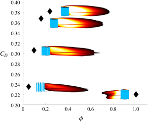
Figure 5. Normalized velocity deficit,  $(u_{bl}-u)/U_{H/2}$, where
  $U_{H/2}$ represents the free-stream velocity at the patch mid-height. Panels (a–f) represent the deficit behaviour for
  $\unicode[STIX]{x1D719}=0.0175,0.05,0.0975,0.16,0.2375,1$, respectively.
In order to visualize the velocity disturbance induced by a porous patch on the incoming boundary layer, a velocity deficit,  $\unicode[STIX]{x0394}u(x,y,z)$, can be defined as the difference between the incoming boundary layer mean velocity profile,
  $u_{bl}(y)$, and the mean streamwise velocity around the body,
  $u(x,y,z)$. The value of
  $\unicode[STIX]{x0394}u(x,y,z)$ is displayed in figure 5(a–f), where the three-dimensionality of the wake can be inferred by combining the mean deficit in both measurement domains. The agreement between datasets is remarkable. Notably, the velocity deficit has been normalized by the undisturbed velocity of the incoming boundary layer at the patch mid-height,
  $U_{H/2}=12~\text{m}~\text{s}^{-1}$; this is an arbitrary normalization factor, nevertheless, it is able to retain some information on the vertical extent of the body. The evolution of the velocity deficit, presented in figure 5(a–f) for increasing
  $\unicode[STIX]{x1D719}$ values (
 $\unicode[STIX]{x1D719}=[0.0175;1]$), allows for the introduction of the main flow features triggered by the permeable nature of the patches. The velocity deficit originates upwind of the body, where the flow deviates and adjusts due to the presence of the body itself. Downwind of the body, the velocity deficit and its spatial evolution are dictated by the drag force and the characteristics of the eddies generated by the patches. Such eddies dominate turbulent momentum transport across the wake and, ultimately, flow recovery in the far field. The contour levels reported in figure 5(a–f) allow for the identification of the planar extent of the wake as the region, past the body, confined by the 20 % of velocity deficit. This means that, at the edge of the coloured regions, the streamwise velocity has recovered 80 % of its undisturbed value upwind of the patch. At a first glance, it is evident that the patch characterized by the lowest
  $\unicode[STIX]{x1D719}$ (figure 5a) shows a sudden wake recovery, articulated in a deficit behaviour pertaining to the recovery of one of the cylinders forming the obstruction. In this case, the wakes of each cylinder within the patch recover individually without mutual interaction, hence preventing the occurrence of a group behaviour. This is in agreement with the findings of Nicolle & Eames (Reference Nicolle and Eames2011), who also report no group behaviour for
  $\unicode[STIX]{x1D719}<0.05$. Therefore, the discussion is from now on restricted to cases
  $C20$,
  $C39$,
  $C64$,
  $C95$, where the wakes of individual elements significantly interact. The solid cylinder (i.e.
  $\unicode[STIX]{x1D719}=1$) is used as a benchmark as it represents a widely investigated condition (Sumner Reference Sumner2013). Globally, figure 5(b–f) is indicative of how a reduced density,
  $\unicode[STIX]{x1D719}=(0.05{-}0.24)$, results in a wake radically different to that of a solid body in extent and flow behaviour, consistent with the work of Castro (Reference Castro1971) who examined the wake of two-dimensional (2-D) perforated plates. This is also reflected in the value of the drag coefficient, which is higher that the one of the solid body for most of the investigated densities (Taddei et al. Reference Taddei, Manes and Ganapathisubramani2016).
The size of the wake can be quantified by a characteristic vertical,  $H_{W}$, and longitudinal,
  $L$, extents (see as reference figure 6):
  $H_{W}$ is the maximum wall-normal distance reached by the wake edge, as detected on the vertical plane;
  $L$ is the maximum distance covered in the streamwise direction, as detected on the horizontal plane spanning eight patch diameters. As already mentioned, the threshold applied to quantify the wake extent was set to 0.2. This is an arbitrary level allowing for the edge of the wake to be included at least in one of the two fields of view. In the spirit of lowering the arbitrariness of this choice, the effect of the threshold value on the detected extent was tested: a variation of ±10 % in the threshold causes maximum variations of ±1.8 % and ±6 % in the vertical and horizontal length scales, respectively, as denoted in figures 7(c) and 7(d) by the symbols (crosses). Not surprisingly, the vertical extent of the wakes is essentially dictated by the height of the patch, regardless of whether the patch is porous or solid. Considering the porous cases only, the influence of the density on the wakes’ vertical extent is limited to variations of approximately 30 % and can be explained as an effect of the vertical bleeding, which, essentially, expands the wake upwards. In order to provide a more quantitative picture and to corroborate this hypothesis, we define vertical bleeding as the integral average of the wall-normal velocity component at the top of the patch:
  $v_{bleed}=2/(0.5D)\int _{0}^{D/2}v(x,H)\,\text{d}x$;
  $v_{bleed}$ is reported in figure 7(a), which shows how
  $v_{bleed}$ increases with increasing
  $\unicode[STIX]{x1D719}$. As reported in figure 7(c),
  $H_{W}$ also increases with increasing density, hence confirming that vertical bleeding and
  $H_{W}$ are closely related.

Figure 6. Sketches of wake height and length in panels (a) and (b), respectively.
The longitudinal extent  $L$ pertaining to the wakes of the porous patches is locked between approximately
  $5$ and
  $7$ diameters downwind of the patches, with a slight maximum for
  $C39$ and the lowest value for
  $C95$. In contrast, the wake of the solid cylinder recovers much faster, within
  $2$ patch diameters only. The behaviour of the recovery length of the porous patches can be explained in terms of vertical and trailing edge bleeding. Towards this end, we quantify the trailing edge bleeding as the integral average of the longitudinal velocity component across the entire height of the patch, i.e.
  $u_{bleed}=1/(H)\int _{0}^{H}u(D/2,y)\,\text{d}y$, (see figure 7b).

Figure 7. (a) Vertical bleeding at increasing density. (b) Horizontal bleeding at increasing density. (c) Vertical wake extent,  $H_{W}$, as a function of
  $\unicode[STIX]{x1D719}$ (the crosses bounding the symbols refer to the sensitivity of the wake extent to the threshold level (=20 %) defining the wake edge). (d) Wake length,
  $L$, as detected on the horizontal plane at mid-height.
From a phenomenological point of view, both the trailing edge and vertical bleeding can be thought as mechanisms that prevent wake entrainment (i.e. wake recovery) and therefore promote large values of  $L$. In particular, the trailing edge bleeding contributes to weakening of the intensity of the shear layers forming at the edges of the patch whereas the vertical bleeding contributes to the displacement of the top shear layer away from the core of the wake. Figure 7 shows that, while
  $\unicode[STIX]{x1D719}$ increases, the trailing edge and vertical bleeding decreases and increases, respectively. This behaviour translates into a trade-off mechanism that contributes to set the extent of the wake in a complex way, as detailed in §§ 3.1 and 3.2. For the specific patch geometry presented here (
 $H/D=1,d/D=0.05,N_{c}=7{-}95$), the trade-off mechanism results in an almost constant
  $L$. Indeed, for a given
  $\unicode[STIX]{x1D719}$, the intensity of the bleeding velocities can be altered by changing
  $H/D$ even if the variation is proven to be less relevant compared to that induced by a change in
  $\unicode[STIX]{x1D719}$ (Zhou & Venayagamoorthy Reference Zhou and Venayagamoorthy2019). It should be pointed out that lateral bleeding may also play an important role in the game of wake recovery as it contributes to the lateral displacement of the shear layers forming at the sides of the patches, hence working against wake recovery. While the limited horizontal extension of the PIV measurements presented herein does not allow a reasonable quantification of lateral bleeding (which could be defined as the integral average of the lateral velocity over the patch height at the sides), Taddei et al. (Reference Taddei, Manes and Ganapathisubramani2016) argued that, as far as the wake structure is concerned, lateral bleeding played an important role in defining the separation point around the sides of the patch, which seemed to be fixed regardless of patch density, meaning that, its role in the trade-off mechanism outlined above might be not so important. Clearly, this is just an hypothesis that must be substantiated by further work. It is also worth pointing out, however, that any
  $\unicode[STIX]{x1D719}$ effect on lateral bleeding should be qualitatively similar to that observed for the vertical bleeding (i.e. an increasing trend) hence leading to the same effects in terms of wake recovery. This hypothesis is somewhat supported by the results obtained by Nicolle & Eames (Reference Nicolle and Eames2011) who performed 2-D DNS of flows through arrays with different densities. These simulations are not entirely representative of the flows investigated herein as they pertain to 2-D arrays which are not subjected to free-end effects along the vertical direction, yet they provide qualitative support for the argument outlined above. Furthermore, the non-monotonic behaviour of
  $L$ with
  $\unicode[STIX]{x1D719}$ could be symptomatic of a regime transition between
  $C39$ and
  $C64$, which is also reflected in the levelling off of the drag coefficient reported in Taddei et al. (Reference Taddei, Manes and Ganapathisubramani2016). According to Nicolle & Eames (Reference Nicolle and Eames2011),
  $\unicode[STIX]{x1D719}>0.15$, model
  $C64$ in this case, marks the solid body limit. While this is not the case, as we observe a non-null bleeding and a wake consistently longer that that pertaining a solid body, Zong & Nepf (Reference Zong and Nepf2012) observed a low- to high-flow blockage transition at
  $\unicode[STIX]{x1D719}>0.1$. Such a transition can indeed be responsible for the trend of
  $L$ with
  $\unicode[STIX]{x1D719}$: the presence of a recirculation bubble for
  $C64$ and
  $C95$ is consistent with this hypothesis.
Within the context of two-dimensional flows, in a fairly recent study, Zong & Nepf (Reference Zong and Nepf2012) report experimental results on flows around patches of cylinders piercing the free surfaces of open channel flows. They identified the shear layers growing from the sides of the body as the key mechanisms by which to describe the entire structure of the patches’ wakes. As already pointed out, the present work is an effort to push the study of the flow past porous obstructions towards a more complex case, which includes an extra shear layer forming at the top of the patch. Therefore, the above-referenced work constitutes a benchmark for data comparison and for isolating the effects of the top shear layer on the general wake structure, whose scaling and structure are described in detail in the next sections of the paper.
3.1 Velocity deficit and wake topology on the vertical plane
The behaviour of the velocity deficit, in the wall-normal plane, helps to capture the effects of the top shear layer on the wake’s structure. Figure 8 reports the non-dimensional velocity deficit as a function of the non-dimensional longitudinal ( $x/D$) and vertical (
 $y/H$, see colour bar) coordinates. For any line of constant
  $y/H$, the deficit first increases and then drops towards zero, i.e. the undisturbed condition. The maximum deficit value is strongly dependent on the patch’s density, so that the higher the density the more intense is the deficit. This translates into a sharper and higher deficit peak at increasing
  $\unicode[STIX]{x1D719}$ for all of the assessed wall-normal positions. As pointed out by Zong & Nepf (Reference Zong and Nepf2012), the occurrence of velocity deficit maxima in figure 8 suggests that the wake longitudinal extent,
  $L$, can be described as the sum of two characteristic length scales: the location of the maximum identifies
  $L_{1}$ and the location where wake recovery occurs identifies
  $L_{2}=L-L_{1}$; the flow region contained within
  $L_{2}$ is herein referred to as the near-wake region whereas the flow region upwind of the deficit maximum (i.e.
  $L_{1}$) is referred to as the very-near-wake region. This region is also referred in Zong & Nepf (Reference Zong and Nepf2012) as the steady-wake region, given the constant trend shown by the longitudinal velocity profile.

Figure 8. (a–e) Lines refer to the evolution of the velocity deficit,  $\unicode[STIX]{x0394}u(y)$, at specific wall-normal locations,
  $y/H=[0.1;0.9]$, as identified by the colour code reported at the side of the bottom panel. Symbols highlight the maximum deficit and hence
  $L_{1}$.

Figure 9. Curves described by the maximum velocity deficit location  $L_{1}$ in the wall-normal plane for the assessed densities.
The velocity deficit behaviour in the steady-wake region depends on the flow deceleration occurring before and within the patch. This is taken into account via the non-dimensional flow blockage parameter  $C_{d}aD$ (Rominger & Nepf Reference Rominger and Nepf2011). In particular, according to the level of flow blockage experienced by the flow, Zong & Nepf (Reference Zong and Nepf2012) and Chen et al. (Reference Chen, Ortiz, Zong and Nepf2012) derive predictive models to quantify the patch exit velocity (analogous to the trailing edge bleeding),
  $L_{1}$ and
  $U_{1}$. Avoiding any assumption on
  $C_{d}$,
  $C64$ and
  $C95$ can be considered high-flow blockage canopies, due to the presence of a recirculation bubble in their wake. We observe that the values measured for
  $u_{bleed}/U_{H/2}$ are similar to what is reported in Chen et al. (Reference Chen, Ortiz, Zong and Nepf2012) across the regime transition. This agreement implies that, in 2-D as in three-dimensional (3-D) conditions, the flow adjustment within the patch depends on the level of blockage; however, the lack of a steady-wake region, its extent (
 $L_{1}$) and wall-normal variation, are the result of the three-dimensionality induced by the depth of submergence.
Along the body height, for every given  $\unicode[STIX]{x1D719}$,
  $L_{1}$ describes a curve, enveloping the very-near-wake region, which is reported in figure 9. Not considering some wall proximity effects which promote a reduction in
  $L_{1}$ close to the wall, figure 9 suggests the presence of two distinct zones along the patch vertical extent,
  $y/H$, for cases
  $C20{-}C95$. The edge of the deceleration region (
 $L_{1}$) shows a constant trend until a certain height (
 $y^{\ast }(\unicode[STIX]{x1D719})/H$), with an evident plateau for
  $C64$–
 $C95$, followed by a linear trend toward the top. The value of
  $\unicode[STIX]{x1D719}$ sets the streamwise location and the extent of the plateau: at increasing density, the streamwise location,
  $k$, identifying the plateau, decreases, while
  $y^{\ast }(\unicode[STIX]{x1D719})/H$ shifts progressively closer to the patch top. This double behaviour is well captured by the following relations:
 $$\begin{eqnarray}\displaystyle & \displaystyle \frac{L_{1}}{D}=m\frac{y}{H}\quad \text{for }\frac{y}{H}>\frac{y^{\ast }}{H}, & \displaystyle\end{eqnarray}$$
 $$\begin{eqnarray}\displaystyle & \displaystyle \frac{L_{1}}{D}=k\quad \text{for }\frac{y}{H}<\frac{y^{\ast }}{H}, & \displaystyle\end{eqnarray}$$
 where  $m=-3.06$ and
  $k=2.6,2.48,1.94,1.47$ for experiments
  $C20$,
  $C39$,
  $C64$ and
  $C95$, respectively. It is worth mentioning that the location where the change in the trend occurs,
  $y^{\ast }/H$, acts as a sort of equivalent patch height: below
  $y^{\ast }/H$, the wake development is influenced by density, above is independent.
3.2 Interplay between shear layers
In order to understand the meaning of the double behaviour of  $L_{1}$, it is worth speculating on the mechanisms driving the recovery of the velocity deficit in the very-near-wake region. The drag force the patch exerts on the impinging flow relates to a pressure gradient between the patch front and rear, which, in turn, drives the trailing edge bleeding over a vertical extent matching the patch height (
 $H$) quantified by
  $u_{bleed}$ as defined at the beginning of § 3 and displayed in figure 7(b) for all of the assessed
  $\unicode[STIX]{x1D719}$. Immediately downwind of the patch, at a height matching the patch vertical extent, the bleeding current comes into contact with the faster, almost undisturbed, flow overlying the patch, and a top mixing layer develops across the wall-normal direction (see e.g. figure 10a). The bleeding velocity,
  $u_{bleed}$, and the streamwise velocity at
  $x=0.5D$ and
  $y=1.1H$,
  $u_{1.1H}$, provide the characteristic velocity scales of the mixing layer. Referring to the sketch in figure 11(a), these are as follows: the convective velocity,
  $U_{c}=0.5(U_{2}+U_{1})=0.5(u_{1.1H}+u_{bleed})$, and the velocity difference,
  $(U_{2}-U_{1})=(u_{1.1H}-u_{bleed})$. Figures 11(b) and 11(c) display the ratio of the characteristic scales and the magnitude of the Reynolds shear stress as functions of
  $\unicode[STIX]{x1D719}$. Within the mixing layer, the velocity discontinuity generates intense turbulence levels, as captured by the Reynolds shear stress profiles shown in figure 10 for model
  $C39$, which is representative of the general trend observed for all tested densities. The centre of the mixing layer can be identified as the inflection point of the velocity profiles or by the location of the peak in the Reynolds shear stress profiles (figure 10b). Along the longitudinal coordinate, the mixing layer enlarges by attenuating the velocity discontinuity and diffusing the Reynolds shear stress peaks.

Figure 10. (a) Map of the Reynolds shear stress, reported as  $-u^{\prime }v^{\prime }/U_{H/2}^{2}$ for display purposes, for model
  $C39$, assuming this is representative of the general trend. (b) Symbols represent the velocity deficit evolution downstream the patch in sections
  $x/D\approx (0.5,0.75,1,1.25,1.5,1.75,2,2.25,2.5,2.75,3)$ (as marked by the grey lines on the top map), superimposed on the Reynolds shear stress profiles (lines) at the same locations.

Figure 11. (a) Schematic of the shear layer forming at the top of the body. (b) Typical velocity difference normalized by the convective velocity,  $U_{c}=0.5(U_{2}+U_{1})$. (c) Shear layer magnitude,
  $\max (-u^{\prime }v^{\prime })/U_{2}^{2}$, as absolute maximum in the wall-normal plane. (d) Mixing layer edge
  $y_{1}$.
As depicted in figure 11, the upper and lower edges of the mixing layer are identified by  $y_{2}$ and
  $y_{1}$, respectively, which in turn are defined as the vertical locations where the Reynolds shear stress reaches 10 % of its maximum value for each given streamwise location (see sketch in figure 11a). Based on a contiguity principle, the lower edge,
  $y_{1}$, is presumably more directly connected to the behaviour of
  $L_{1}$ than
  $y_{2}$ and therefore is herein further analysed.
Figure 11(d) shows that, with increasing longitudinal distance,  $y_{1}$ decreases linearly for the less dense cases (i.e.
  $C20$ and
  $C39$), hence suggesting a linear growth of the mixing layer width (as expected for a plane mixing layer; see Patel (Reference Patel1973) and Champagne, Pao & Wygnanski (Reference Champagne, Pao and Wygnanski1976)). In contrast, for the more dense patches,
  $y_{1}$ first shows a nonlinear behaviour in the patch proximity, followed by a linear trend. At
  $x/D\geqslant 3$,
  $y_{1}$, for
  $C39$–
 $C95$, collapses, suggesting that the mechanisms responsible for the bending of the shear layers are no longer effective.

Figure 12. (a) Schematic of the shear layer forming at the sides of the body. (b) Normalized velocity difference at increasing  $\unicode[STIX]{x1D719}$. (c) Mixing layer edge
  $z_{1}$ for the tested solidities.
The nonlinear behaviour of  $y_{1}$ is associated with a nonlinear growth of the mixing layer, which could have several causes, all ascribable to mechanisms that are not present in canonical plane mixing layers: (i) at increasing
  $\unicode[STIX]{x1D719}$, the increasing vertical bleeding (see e.g. figure 7b) pushes and deforms the shear layer in the region close to the patch top; (ii) the interaction of the top shear layer with the shear layers growing and developing on the sides of the patches; (iii) the occurrence of a separation bubble. As for the wall-normal plane, on the horizontal plane, the inner edge of the shear layer can be defined as the spanwise location where, at each longitudinal position
  $x$, the Reynolds stress
  $u^{\prime }w^{\prime }/U_{H/2}^{2}$ reaches 10 % of its maximum value. The value of
  $z_{1}$, detected for each patch density, is depicted in figure 12 together with the typical velocity scales. Here, as well for the higher densities, the shear layer growth does not seem to be linear, probably for the same reasons discussed for the top shear layer.
This is at odds with the experimental results reported by Zong & Nepf (Reference Zong and Nepf2012) for two-dimensional flow conditions (i.e. patches piercing the free surfaces of impinging open channel flows, namely when  $\unicode[STIX]{x1D6FF}/H=1$), who argued that the mixing layer growth at the sides of the patches was essentially linear. Since the difference between the experiments presented herein and those by Zong & Nepf (Reference Zong and Nepf2012) is the occurrence of a top shear layer, it is reasonable to speculate that, among all of the possible causes of nonlinearity in the mixing layer growth listed above, the (mutual) interaction between the top and lateral shear layers may be the dominant one.
Among various other results, Zong & Nepf (Reference Zong and Nepf2012) also argued that the location where the horizontal shear layers merge coincides, within experimental uncertainty, with the location where the velocity deficit reaches its maximum, hence offering an alternative definition for  $L_{1}$. On the basis of this assumption and of a symmetrical growth of the shear layers, the expected value for the location of the maximum velocity deficit would be
  $L_{1,exp}=-0.5D/(\text{d}z_{1}/\text{d}x)$. In the experiments by Zong & Nepf (Reference Zong and Nepf2012), where
  $z_{1}$ shows a linear development, the expression for
  $L_{1,exp}$ can be recast as
  $L_{1,exp}=-0.5D/(S(U_{2}-U_{1})/U_{c})$, where
  $S=(\text{d}z_{1}/\text{d}x)((U_{2}-U_{1})/U_{c})$ (commonly referred to as the spreading parameter) is independent of the typical velocity scale (Pope Reference Pope2000) and can be estimated approximately as
  $S=(0.06{-}0.11)$ for cylinders (Champagne et al. Reference Champagne, Pao and Wygnanski1976; Dimotakis Reference Dimotakis1991),
  $S=0.073$ for a plate and
  $S=0.103$ for a flat plate (Pope Reference Pope2000).

Figure 13. Comparison between  $L_{1}$, location of the maximum deficit, and
  $L_{1,exp}$, location where the horizontal shear layers merge (symbols); the line marks the
  $L_{1}$ for 2-D conditions, namely the 1 : 1 line agreement.
In the present investigation, in three-dimensional flow conditions ( $\unicode[STIX]{x1D6FF}/H>1$), the mutual interaction between the top and horizontal shear layers, produces a curvature in the detected
  $z_{1}$, so as neither equation for
  $L_{1,exp}$ provides a good estimation. As a matter of fact, the estimated value for
  $\text{d}z_{1}/\text{d}x$, by means of a linear regression, would represent a severe approximation due to the curvature of
  $z_{1}$ as the ratio of the typical velocity scales is no longer uniquely responsible for the shear layer spreading. For these reasons, an expected value for
  $L_{1}$ can be obtained directly from the trend of
  $z_{1}$. The value of
  $L_{1,exp}$, in fact, coincides with the
  $x/D$ location where the growth of the inward edge of the horizontal shear layer,
  $z_{1}$, stops, due to its merging with the
  $z_{1}$ edge of the symmetric shear layer (not shown in figure 12). The expected value
  $L_{1,exp}$ is compared to
  $L_{1}$, as detected from the deficit profiles, in figure 13. Here, it is evident that
  $L_{1}$ does not match the location where the horizontal shear layers merge. In figure 13, the distance between the baseline and the symbols quantifies the discrepancy. The value of
  $L_{1,exp}$ clearly exceeds the
  $L_{1}$ value for all the densities due to the recovery effect accomplished by the top mixing layer, which conveys faster flow toward the wall and provides an enhanced turbulence level to cancel out the deficit. The mutual interaction between top and horizontal shear layers can also provide some insights to explain the trend described by
  $L_{1}$ along the entire patch height, as reported in figure 9. Close to the top of the patch, where
  $L_{1}$ shows a consistent linear behaviour for all densities, the top mixing layer is probably the dominant recovery mechanism and the proportionality between its intensity and the velocity deficit to be recovered (see e.g. figures 11b and 11c) cancels out the dependence on
  $\unicode[STIX]{x1D719}$. Moving down toward the wall, the vertical shear layer progressively attenuates and interacts with the horizontal ones. This interaction concurs with a mutual bending and is the origin of the constant trend observed for
  $L_{1}$. In the spirit of generalizing this argument, it is worth mentioning that the relative position of the shear layers depends on patch height and diameter, hence changing
  $H/D$ is expected to impact the shape of the very-near-wake region.
3.3 Wake scaling on the horizontal plane

Figure 14. Velocity deficit evolution on the horizontal plane at the body mid-height; the increasing density corresponds to cases  $C7,C20,C39,C64,C95,CS$.

Figure 15. Evolution of velocity deficit profiles at increasing density: (a)  $C20$; (b)
  $C39$; (c)
  $C64$; (d)
  $C95$.
In figure 14 the evolution of the non-dimensional velocity deficit  $\unicode[STIX]{x0394}u/U_{H/2}$, defined as the difference between the incoming streamwise velocity at the patch mid-height,
  $U_{H/2}$, and the velocity profile,
  $u(x,z)$, at each longitudinal location, is summarized for all patch densities in several sections (
 $x/D=[1:8]$) downwind of the patches. At
  $x/D=1$, it is evident how the velocity profiles pertaining to the porous patches differ from that pertaining to a solid body (black continuous line). The deficit induced by the presence of the solid body has an intensity comparable to that of the intermediate density case,
  $C39$; it extends in the spanwise direction in the range
  $(-0.5:0.5)D$, while the deficit for the patches is in the range
  $(-1:1)D$. At this streamwise location, the velocity deficit pertaining to the solid body is already decaying, having reached its maximum at
  $x/D(=L_{1})\approx 0.7$, while the deficit of the porous patches is increasing. For
  $x/D=[2:8]$, the deficits of the patches evolve, suggesting a preservation in the shape, as will be discussed in the next paragraphs, and, notably, for
  $x/D>4$, the velocity profiles of
  $C20$–
 $C95$ are almost indistinguishable. This would suggest that, across the near wake, the velocity deficit becomes independent of density and this will be eventually reflected in the law describing the deficit decay. The decay and the spread of the velocity profiles along
  $x/D$ resembles the evolution of a plane wake. This is true despite the fact that key assumptions required for self-similarity to occur are violated, namely, the wall-normal component is not null and the ratio between the maximum velocity deficit,
  $\unicode[STIX]{x0394}u(x,z=0)$, and the convective velocity,
  $U_{H/2}$ (i.e. the free-stream velocity), is larger than 0.1, the value at which self-similarity is usually observed in the experiments (Pope Reference Pope2000). In general, the disturbance induced by a plane wake generator is defined as a characteristic velocity difference between the incoming uniform stream and the flow past the body. In the case of a plane wake, the velocity deficit evolves in the field, reaching a self-similar state (Pope Reference Pope2000) that is controlled by two typical velocity and length scales, which depend only on the longitudinal coordinate
  $x$. In the present case also the patch density
  $\unicode[STIX]{x1D719}$ should be taken into consideration so that
 $$\begin{eqnarray}\unicode[STIX]{x0394}u(x,z,\unicode[STIX]{x1D719})=\unicode[STIX]{x0394}u_{0}(x,\unicode[STIX]{x1D719})f(z/z_{1/2}(x,\unicode[STIX]{x1D719})).\end{eqnarray}$$
 In this equation,  $\unicode[STIX]{x0394}u_{0}(x,\unicode[STIX]{x1D719})=U_{H/2}-u(x,0,\unicode[STIX]{x1D719})$ is the velocity scale, representative of the maximum velocity deficit at each streamwise location, with
  $u(x,0,\unicode[STIX]{x1D719})$ the minimum that the velocity reaches in correspondence with
  $z/D=0$, which corresponds to a maximum in
  $\unicode[STIX]{x0394}u$;
  $z/z_{1/2}$ is the self-similar cross-stream variable, where
  $z_{1/2}$, namely the wake half-width, is the
  $z$ location where the velocity deficit falls to half of its maximum value;
  $f(z/z_{1/2}(x,\unicode[STIX]{x1D719}))$, the self-similar velocity defect, qualifies the wake spread and decay.
Figure 15(a–d) shows the velocity deficit profiles, for cases  $C20$–
 $C95$, normalized by the characteristic velocity scale (
 $\unicode[STIX]{x0394}u_{0}$), against the lateral coordinate, normalized by the characteristic length scale (
 $z_{1/2}$), for several longitudinal locations past the patches. For almost all of the assessed densities, past the steady-wake region (
 $x/D>L_{1}$), the deficit profiles show a remarkable collapse along
  $x/D$ for almost the entire spanwise extent of the wakes except for the tails.

Figure 16. (a) Deficit profiles at  $x/D=3$ for cases
  $C20$–
 $C95$ (markers) scaled up with the characteristic velocity and length scale,
  $\unicode[STIX]{x0394}u_{0}$ and
  $z_{1/2}$; solid lines represent the least squares fitting of data through
  $f=\text{e}^{-\unicode[STIX]{x1D6FC}(z/z_{1/2})^{2}}$. (b, top) The
  $\unicode[STIX]{x1D6FC}$ parameter in several downstream locations compared to the typical value for a 2-D wake
  $\unicode[STIX]{x1D6FC}\approx 0.693$. (b, bottom) Goodness of fit as the root mean square error (RMSE).


In figure 16(a) the decay of the velocity deficit for  $C20{-}C95$ at
  $x/D=3$, is reported. For self-preserving wakes, the velocity defect scales according to an exponential law
 $$\begin{eqnarray}f(z/z_{1/2})=\exp (-\unicode[STIX]{x1D6FC}(z/z_{1/2})^{2}),\end{eqnarray}$$
 where  $\unicode[STIX]{x1D6FC}_{2-D}=\ln (2)\approx 0.693$ for the wake of two-dimensional obstacles. The lines superimposed on the scaled profiles in figure 16(a) represent the self-similar velocity defect at
  $x/D=3$ resulting from a fitting procedure of (3.4), where
  $\unicode[STIX]{x1D6FC}$ is the free parameter. The good agreement, for
  $z/z_{1/2}$ spanning the range
  $[-1;1]$, between the scaling provided by the self-similar velocity defect and the measured evolution, can be visually assessed in figure 16(b) for
  $x/D=3$. The same fitting procedure for different values of
  $x/D$ allows us to compute a root mean square error that shows to what extent the scaling of the velocity defect deviates from its canonical 2-D counterpart. Results show that
  $\unicode[STIX]{x1D6FC}=\unicode[STIX]{x1D6FC}_{2-D}\pm 10\,\%$, so that the behaviour of the wake of a porous patch can be considered two-dimensional on the horizontal plane at mid height.
3.4 Universal scaling for the wake development
As a result of the self-preserving state of the velocity deficit, on the basis of mean momentum conservation arguments, Wygnanski, Champagne & Marasli (Reference Wygnanski, Champagne and Marasli1986) provide the following scaling laws for both the characteristic length and velocity scales:
 $$\begin{eqnarray}\displaystyle & \displaystyle \frac{\unicode[STIX]{x0394}u_{0}}{U_{H/2}}\propto \left(\frac{x-x_{0}}{C_{D}D}\right)^{-1/2}, & \displaystyle\end{eqnarray}$$
 $$\begin{eqnarray}\displaystyle & \displaystyle \frac{z_{1/2}}{D}\propto \left(C_{D}\frac{x-x_{0}}{D}\right)^{1/2}, & \displaystyle\end{eqnarray}$$
 where  $x_{0}$ is a virtual origin, and
  $D$ the patch diameter. The value of
  $C_{D}$, the patch drag coefficient, is displayed in figure 18 over the range of patch densities for which self-similarity is observed. Taddei et al. (Reference Taddei, Manes and Ganapathisubramani2016) have already extensively covered the behaviour of the drag experienced by these patches. In figures 17(a) and 17(b), the detected wake half-width and the maximum deficit are reported against the streamwise coordinate,
  $x/D$, scaled as suggested in (3.5) and (3.6). Surprisingly, a linear behaviour is evident for the characteristic scales already in the near-wake region, namely for
  $x-x_{0}>L_{1}$, consistent with the early self-similarity observed in the deficit evolution. The agreement between (3.5), (3.6) and the detected trend means that, as for a 2-D wake, the deficit is generated when the incoming flow exchanges momentum with the body, resulting in the drag force
  $C_{D}$, which is a function of
  $\unicode[STIX]{x1D719}$; at the same time,
  $C_{D}$ represents the suitable parameter to stretch the wake spreading, taking into account the density. The virtual origin
  $x_{0}$ is defined as the minimum streamwise location where linearity is consistently observed for both the length and the velocity scales. The value of
  $x_{0}$ depends on
  $L_{1}$, since the extent of the very near wake marks the recovery onset, and on the patch-generated turbulence, available for the deficit recovery. In fact, in analogy with the development of a plane wake in presence of free-stream turbulence (see Symes & Fink (Reference Symes, Fink and Fiedler1977)), the increasing density provides an increasing turbulence (see e.g. figure 11c) as a consequence of the intensity of the shear layers forming at the patches’ edges. The enhanced turbulence intensity is responsible for speeding up the recovery.

Figure 18. Value of  $C_{D}=F/0.5\unicode[STIX]{x1D70C}D^{2}U_{\infty }^{2}$, as a function of
  $\unicode[STIX]{x1D719}$, as measured in Taddei et al. (Reference Taddei, Manes and Ganapathisubramani2016).
4 Conclusions
This paper investigates the scaling of the wake shed by arrays (i.e. patches) of cylinders impinged by a turbulent boundary layer. Experiments were carried out by extensively varying the array density ( $\unicode[STIX]{x1D719}=0.0175{-}0.2375$) and by keeping the impinging boundary layer (
 $\unicode[STIX]{x1D6FF}$) deeper than the height (
 $H$) of the patch (
 $\unicode[STIX]{x1D6FF}/H=3.58$). The flow field within the wakes was explored by wall-normal and wall-parallel two-dimensional PIV measurements. Results were put into the context of recent literature focusing on open channel flows impinging cylinder arrays piercing the free surface, as they represent a two-dimensional benchmark to disentangle the complex three-dimensional flow features explored herein. The main results of this study can be summarized as follows.
The size of the wakes shed by the porous arrays is far greater than the wake of their solid counterparts. This is an effect caused by the bleeding flow occurring at the edge of the arrays, which contributes to increase the extent of the wakes. It was also observed that the velocity deficit reaches a maximum over  $L_{1}$, which was referred to as the very-near-wake region. Beyond this region the wake would undergo an effective recovery over a length
  $L_{2}=L-L_{1}$.
The difference in height between the impinging flow and the arrays is responsible for the generation of a top mixing layer, which interacts with the mixing layers forming at the sides of the arrays. The interaction results in a nonlinear growth of the mixing layers for higher densities. Interestingly, on the horizontal plane at the patch mid-height, the velocity deficit recovers in a self-similar fashion, resembling the behaviour of a canonical planar wake. Consistently, the characteristic velocity and length scales describing the self-similarity of the mean flow appear to approximately follow the classical scaling of a planar wake. The virtual origin of the self-similarity appears to depend on the patch density and, once this accounted for, the wakes exhibit approximate self-similarity.
Finally, the observed mean flow self-similarity could be useful to predict the flow in the wake of porous bodies organized in arrays (such as turbines and/or cluster of buildings) where the layout dictates the performance. The model provides estimates for the wake relaxation length and velocity deficits despite the fact that the flow is three-dimensional in the near wake due to bleeding in the vertical and horizontal directions.
Acknowledgements
We gratefully acknowledge the funding from EPSRC (grant ref no. EP/P021476/1). C.M. acknowledges support from Compagnia di San Paolo through the project ‘Attrarre Docenti di qualitá tramite Starting Grant’. Data published in this article are available from the University of Southampton repository at https://doi.org/10.5258/SOTON/D1274.
Declaration of interests
The authors report no conflict of interest.


