


1. Introduction
1.1. Background and objectives
Entrainment is the process that enables the growth and spread of turbulent shear flows. Because of its importance for many engineering and geophysical applications, the physics of turbulent entrainment have been thoroughly investigated. A concept that has commonly been used in studies of entrainment and growth of turbulent shear flows is the existence of a turbulent/non-turbulent interface (TNTI), which separates the regions of turbulent flow from those of non-turbulent flow. Corrsin & Kistler (Reference Corrsin and Kistler1955) postulated two important hypotheses: (i) that there is a step-like change in velocity across the TNTI, and (ii) that the spreading process of turbulence into the non-turbulent flow region is similar to turbulent diffusion, a process that has been commonly referred to as ‘nibbling’. The first point indicates that the TNTI is typically sharp, with a thickness of approximately one to two orders of magnitude smaller than the integral flow scale (Chevray Reference Chevray1982; Bisset, Hunt & Rogers Reference Bisset, Hunt and Rogers2002; Hunt, Eames & Westerweel Reference Hunt, Eames and Westerweel2006). The latter point suggests that engulfment, which is the name given to the process where large eddies draw fluid from the non-turbulent region into the turbulent flow (Brown & Roshko Reference Brown and Roshko1974; Townsend Reference Townsend1976), does not play a major role in the entrainment process. Townsend (Reference Townsend1976) disagreed with Corrsin & Kistler's (Reference Corrsin and Kistler1955) second hypothesis and claimed that the bulk motion is sufficient to determine the wake spreading and entrainment rates in free shear flows.
Within the core of turbulent shear flows, there is typically a region where the flow is fully turbulent. For example, for the far field of plane turbulent wakes, the intermittency factor, which is the proportion of time that the flow is turbulent at a point, is unity for  $y/y_{1/2} < \approx 1$ (Kopp, Giralt & Keffer Reference Kopp, Giralt and Keffer2002), where
  $y$ is the distance from the centreline and
  $y_{1/2}$ is the mean velocity half-width. For distances further from the centreline, the turbulent flow is intermittent and is made up of turbulent bulges of varying sizes. LaRue & Libby (Reference LaRue and Libby1974) found that the bulges are consistent with the three-dimensional double roller vortices first proposed by Grant (Reference Grant1958). Thus, Corrsin & Kistler's (Reference Corrsin and Kistler1955) velocity step change across the TNTI is connected to the coherent structures (CS) in the flow field. Further, Kopp et al. (Reference Kopp, Giralt and Keffer2002) found that (i) the bulges are, in fact, made up of the both the three-dimensional horseshoe/double roller vortices and a region of high strain in the region immediately upstream of these vortices, and that (ii) the shape of the interface depends on this structure with the upstream edge being shear-aligned while the downstream edge is not. This implies that the growth or spread of the plane turbulent wake, as indicated by the evolution of the TNTI is controlled by the nature of the CS within the turbulent bulges.
However, the historical disagreement regarding the mechanism of entrainment remains. For example, more recent studies (e.g. Mathew & Basu Reference Mathew and Basu2002; Westerweel et al. Reference Westerweel, Fukushima, Pedersen and Hunt2005; Holzner et al. Reference Holzner, Liberzon, Nikitin, Kinzelbach and Tsinober2007; DaSilva & Pereira Reference DaSilva and Pereira2008; Hunt et al. Reference Hunt, Eames, da Silva and Westerweel2011) suggest that nibbling is the main mechanism of entrainment in turbulent jet flow, in agreement with the second hypothesis of Corrsin & Kistler (Reference Corrsin and Kistler1955). Westerweel et al. (Reference Westerweel, Fukushima, Pedersen and Hunt2009) showed that large-scale engulfment would account for less than 10 per cent of the total fluid mass entrained and suggested that the entrainment process is mainly dominated by small-scale nibbling. More recently, Philip & Marusic (Reference Philip and Marusic2012) showed that the mean velocities and second-order statistics in jet and wake flows could be obtained by a large-scale eddy model that they proposed and concluded that the primary cause of entrainment could be the large-scale engulfment, combined with small-scale nibbling.
Thus, while the rate of entrainment of non-turbulent flow into a turbulent shear flow is clearly related to the characteristics of the TNTI, the role of the motions present in the turbulent region near the TNTI remains unclear. Given these discrepancies, it appears that entrainment must be flow dependent. The purpose of the paper is to examine this issue, i.e. to determine the role of flow-dependent CS in controlling the entrainment rate and the mechanisms of nibbling and engulfment. To achieve this, we develop a three-dimensional flow based on careful modifications to the flow field of the circular cylinder, as discussed next.
1.2. Role of CS in entrainment for plane turbulent wakes
The wake behind a circular cylinder is an ideal flow system to study the genesis of large-scale structures and their dynamical evolution with respect to initial flow conditions. Numerous numerical and experimental studies have been carried out in the past to characterize the large-scale structures in the near-, mid- and far-wake regions. Early classical works investigated the vortex street (Kármán & Rubach Reference Kármán and Rubach1912) and the variation of drag of cylinders with aspect ratio (Taylor Reference Taylor1915). Flow instability and transitions in the near wake have been studied by many researchers (e.g. Gerrard Reference Gerrard1967; Roshko & Fiszdon Reference Roshko and Fiszdon1969; Zdravkovich Reference Zdravkovich1990; Williamson Reference Williamson1996; Norberg Reference Norberg2003). Cantwell & Coles (Reference Cantwell and Coles1983) used flying hot-wire devices together with phase averaging techniques to obtain conditional averages of normal and shear stresses, intermittency, vorticity and velocities in the near turbulent wake of a circular cylinder at a Reynolds number of  $Re = 1.4 \times 10^5$. The Reynolds number is defined as
  $Re=U_0 D / \nu$, where
  $U_0$ is the free-stream velocity,
  $D$ is the cylinder diameter and
  $\nu$ is the fluid (air) kinematic viscosity.
These authors concluded that the mechanism of turbulence production was likely to be vortex stretching at intermediate scales. Entrainment was also found to be closely associated with saddles located between the Kármán vortices, where the maximum value of random shear stress, which is not related to the von Kármán vortices, occurs, suggesting the presence of other three-dimensional structures in the near wake. These three-dimensional structures were later observed by Hayakawa & Hussain (Reference Hayakawa and Hussain1989).
Hayakawa & Hussain (Reference Hayakawa and Hussain1989) observed the presence of three-dimensional organized structures in the von Kármán vortex street in the near and mid–far wake, ( $10 \le x/D \le 40$;
  $x$ is the streamwise coordinate) at a Reynolds number of
  $Re=13\,000$. These authors employed a methodology based on the detection of vorticity peaks in the hot-wire time histories. They reported that the von Kármán vortices (VKV) could be interconnected with secondary vortices having streamwise vorticity. Ferré & Giralt (Reference Ferré and Giralt1989a), using a pattern recognition approach, analysed the evolution of large-scale organized motions in the range
  $10 \le x/D \le 40$ at
  $Re = 9000$. They found and that the periodic activity of the Kármán vortices persists up to 60 diameters downstream. Yamane et al. (Reference Yamane, Oshima, Okubo and Kotani1988) analysed the wake behind a circular cylinder at
  $Re=2100$ and
  $4200$, using a flow visualization technique and simultaneous hot-wire measurements. They reported the predominance of Kármán vortices at
  $x/D=10$, the presence of a complex flow field near
  $x/D=60$, where transition from Kármán vortices to some new CS takes place, with far-wake large-scale structures that are formed by
  $x/D=90$. More recently, the direct numerical simulations carried out by McClure, Pavan & Yarusevych (Reference McClure, Pavan and Yarusevych2019) showed that Kelvin–Helmholtz instabilities led to the formation of hairpin structures in the near wake for
  $Re \ge 800$ when streamwise vortex pairs pinch off vorticity from Kármán vortices and reorient to form the legs of hairpins. They reported that this regime is characterized by a significant increase in vortex deformation and a wake flow with a large number of hairpin formations.
The existence of large-scale CS in the turbulent far wake of the cylinder has been known for quite long. More generally, the importance of three-dimensional structures in turbulent wakes was well established by the pioneering works of Theodorsen (Reference Theodorsen1952), Townsend (Reference Townsend1956) and Grant (Reference Grant1958). Theodorsen (Reference Theodorsen1952) proposed that the predominant structure in a developed wake should be a horseshoe-like vortex. Grant (Reference Grant1958) postulated, on the basis of a comprehensive set of correlation measurements in the far wake of a cylinder at  $x/D=533$, the existence of shear-aligned double roller eddies and ‘mixing jets’ as ejections of turbulent flow from the centre of the wake towards the non-turbulent external flow region. Ferré & Giralt (Reference Ferré and Giralt1989a) refined the pattern recognition technique, previously developed by Mumford (Reference Mumford1983), to analyse large-scale motion at
  $x/D=140$. They found that the large-scale flow organization consisted of double roller eddies. Similar double roller-like structures in the far wake were identified later by several researchers (e.g. Ferré & Giralt Reference Ferré and Giralt1989b; Hayakawa & Hussain Reference Hayakawa and Hussain1989; Ferré et al. Reference Ferré, Mumford, Savill and Giralt1990; Kopp, Kawall & Keffer Reference Kopp, Kawall and Keffer1995). In particular, Giralt & Ferré (Reference Giralt and Ferré1993) determined that the double roller structure, i.e. a pair of counter-rotating vortices, is simply a horizontal slice through a horseshoe vortex near the wake half-width. Vernet et al. (Reference Vernet, Kopp, Ferré and Giralt1997) gave further evidence, based on their simultaneous temperature and velocity measurements, that Townsend's and Grant's double roller and mixing jet structures are simply different views of a single flow structure, likely a horseshoe-shaped vortex. Vernet et al. (Reference Vernet, Kopp, Ferré and Giralt1999) identified the complete three-dimensional topology of the large-scale structures by using conditional sampling. They confirmed that the structure shape was similar to a horseshoe vortex. Philip & Marusic (Reference Philip and Marusic2012) proposed a simplified axisymmetric wake model, based on randomly inclined vortical structures, which was able to reproduce the experimental mean velocity and normal and shear stress profiles. The genesis of these large-scale structures present in the far wake should be the secondary hairpin vortices characterized by McClure et al. (Reference McClure, Pavan and Yarusevych2019) in the near wake.
Successful models for plane mixing layer entrainment, with overall rates being determined by the engulfing action of large eddies, were constructed for plane mixing layers (Brown & Roshko Reference Brown and Roshko1974). Dahm & Dimotakis (Reference Dahm and Dimotakis1987) used visualizations and measurements of a scalar concentration in the near field of a jet to show that the entrainment process was dominated by the engulfment of large-scale structures. They also showed that local large scales of the flow can be used to characterize the rate of the entrainment process. Ferré & Giralt (Reference Ferré and Giralt1989b) analysed the organized motions of the temperature field in the wake of a heated cylinder at  $x/D=140$ and from the distribution of colder and warmer spots in vertical and horizontal planes they concluded that the double roller vortices are in fact associated with the large-scale entraining motions in the wake. Ferré et al. (Reference Ferré, Mumford, Savill and Giralt1990) and Giralt & Ferré (Reference Giralt and Ferré1993) argued that horseshoe vortices should play an important role in the momentum transfer as they maintain the correlation between the streamwise and vertical velocity fluctuations (i.e. Reynolds shear stress). According to this scenario, the external fluid is first ingested by the highly stretched and twisted interior turbulent flow pattern (large-scale structures) and is then mixed to molecular level by the action of the small-scale velocity fluctuations (Kopp et al. Reference Kopp, Giralt and Keffer2002).
To summarize, there have been several important observations in the literature. First, CS within turbulent shear flows play an important role in setting the details of the TNTI and the rate of entrainment. Second, CS develop and evolve depending on the initial and boundary conditions of the flow. These two observations imply that the relative importance of the nibbling and engulfment mechanisms depend on the flow conditions and the particular details of the CS. Thus, by controlling the development of the CS, like near wake instabilities leading to the formation of hairpins do in a continuous cylinder (CC) turbulent wake, one should control the extent to which each of the mechanisms contribute to the overall entrainment rate. The key question, then, is how to do that, i.e. how to generate hairpin-like structures with high vorticity under turbulent conditions in the near wake. Our hypothesis is that enhancing vortices in the very near wake that are in alignment with the mean shear will increase the rate of entrainment. The shear alignment is critical since it allows the engulfing mechanism to be maintained for a significant duration because vortex stretching will maintain the vorticity in the CS, while in contrast, a lack of shear alignment allows them to decay. This implies that far-wake-type structures such as the shear-aligned horseshoe vortices should have relatively higher entrainment and growth rates than typical near-wake structures such as VKV, which are not shear aligned. The objective of the paper is to test this hypothesis; namely that shear alignment of CS enhances the entrainment rate by increasing engulfment. To test this hypothesis, we develop what we call a discontinuous cylinder wake, described below, such that relatively intense horseshoe or hairpin vortices are formed much earlier in the wake as a result of a primary instability, increasing the growth rate significantly.
2. Methods
2.1. Approach
To investigate our hypothesis, we developed and examined the wake of a segmented circular cylinder, which we refer to as a discontinuous cylinder (DC). As depicted in figure 1, the DC is defined with two non-dimensional parameters: the ratio of the solid segment length to cylinder diameter,  $L/D$, and the gap between the solid segments,
  $S/D$. The idea here is to choose values of
  $L/D$ and
  $S/D$ such that there is early formation of horseshoe vortices (HSV), as depicted in figure 2, but with a far wake that is two-dimensional in the mean. By forcing the early occurrence of HSV, rather than allowing the normal development of three-dimensional structures in the CC wake, we can examine differences in the overall rates of entrainment. By maintaining a two-dimensional far wake, the self-preserving states between the DC and CC wakes can be compared. Analysis of the self-preserving state provides a framework for the comparison. In particular, if the growth rate of the self-preserving states of the two far wakes are the same, then the difference in wake thickness quantifies the difference in entrainment due to the near DC wake structure.

Figure 1. Sketch of the DC model,  $M_1$, used in BLWTL along with the coordinate system.

Figure 2. Sketch of the flow in the proximity of the DCs.
Several studies have examined the effects of finite cylinder length on the vortex structure in the near wake (e.g. Zdravkovich et al. Reference Zdravkovich, Brand, Mathew and Weston1989; Norberg Reference Norberg1994; Williamson Reference Williamson1996; Zdravkovich et al. Reference Zdravkovich, Flaherty, Pahle and Skelhorne1998; Inoue & Sakuragi Reference Inoue and Sakuragi2008). These studies have found a complex dependence of the near-wake vortices on the aspect ratio,  $L/D$. Of importance for the current study, Inoue & Sakuragi (Reference Inoue and Sakuragi2008) found periodic shedding of HSV for
  $L/D=5$ at
  $Re=300$ using direct numerical simulations. This size compares favourably with the spanwise extent of HSV in the far wake, which Vernet et al. (Reference Vernet, Kopp, Ferré and Giralt1999) found to be about 5
 $D$. This suggests that
  $L/D$ should be similar and, hence, a value of
  $L/D=5$ was chosen.
To obtain a far wake behind the DC that is two-dimensional in the mean, the gap between the solid cylinder segments,  $S$, should not be too large. However, if
  $S$ is too small, the gap may be ineffective in allowing the HSV to form in the near wake. Several direct numerical simulations carried out by Mandava et al. (Reference Mandava, Kopp, Herrero and Giralt2009) at
  $Re = 300$, when designing their experimental set-up, led to the conclusion that
  $S/D=2.5$ and
  $L/D=5$ were optimal to shed HSVs behind each segment of the DC configuration in a synchronized manner. This shedding was confirmed experimentally and reported by these authors to also form in the near wake of the DC for
  $Re=10\,000$, further investigated here. When these rows of HSVs alternating with jet-like flows in the spanwise direction get randomized, as they are advected downstream, these spanwise variations are smeared away by turbulence and the far wake becomes two-dimensional on average, as is also the case in the CC far wake. It should also be noted that, given the intricately variable wake structures that occur for finite cylinders, the additional parameter,
  $S/D$, for the DC could also lead to a rich set of vortical structures. This remains to be explored in future work. We carried out particle image velocimetry (PIV) and hot-wire anemometry (HWA) measurements as well as large eddy simulations (LES) to analyse/characterize the wake growth and entrainment rates in the near and far wake of the DC and the analogous CC at the same
  $Re$.
$Re$.
2.2. Experimental details
Three DC models were used in the current study, as defined in table 1. Two of the DC models,  $M_{1}$ and
  $M_{2}$, were used to carry out the measurements in the near- and intermediate-wake regions (up to
  $x/D=56$) in the Boundary Layer Wind Tunnel Laboratory (BLWTL) at the University of Western Ontario (UWO) and the wind tunnel at Universitat Rovira i Virgili (URV). The discontinuous cylinder configuration, depicted in figure 1, utilized 3 and 5 cylindrical segments in the BLWTL at UWO and URV wind tunnels, respectively. The cylinder diameter was
  $D=0.0163$ m in these two models. A thin steel plate having a thickness of
  $\lambda = 0.815\times 10^{-3}$ m and a width equal to
  $D$ held the cylinder segments together without interfering significantly with the flow between the gaps.
Table 1. Geometrical details of the three DC configurations, wind tunnel specifications and experimental conditions.

To carry out the measurements in the far-wake region,  $70 \le x/D \le 180$, a third DC model (
 $M_{3}$) with seven cylinder segments having a smaller diameter (
 $D=0.0065$ m) was used in order to bring the far wake into the optimal measurement region of the wind tunnel. The thickness of the steel plate in the
  $M_{3}$ model was reduced to
  $\lambda =0.30\times 10^{-3}$ m in order to maintain the
  $D/\lambda$ ratio (see table 1). Since the same free-stream speed was maintained for the
  $M_{3}$ experiments, the Reynolds number in the far wake measurements was lower, as indicated in table 1. The experiments were carried out in an open-return wind tunnel at BLWTL in Canada and in the open-return wind tunnel at URV in Tarragona, Spain. The wind tunnel at BLWTL is of the suction type with a cross-section of
  $0.45\,{\rm m}\times 0.45\,{\rm m}$ and a length of 1.5 m. The intake flow was straightened through a honeycomb and fine screen prior to entering a
  $7.4:1$ contraction. This tunnel was used earlier for wide range of inflow velocities from 1.25 to 17.8 m s
 $^{-1}$ (see e.g. Bailey, Martinuzzi & Kopp Reference Bailey, Martinuzzi and Kopp2002; Martinuzzi, Bailey & Kopp Reference Martinuzzi, Bailey and Kopp2003; Dol, Kopp & Martinuzzi Reference Dol, Kopp and Martinuzzi2008; Taylor et al. Reference Taylor, Palombi, Gurka and Kopp2011). The free-stream turbulence intensity was
  $1\,\%$. The wind tunnel at URV was also of the suction type with a cross-section of
  $0.6\,{\rm m}\times 0.6\,{\rm m}$ and a length of
  $3$ m. A set of flow straighteners and filters and a contraction zone of ratio
  $9:1$ produced a low turbulence (less than
  $0.2\,\%$) for the
  $U_0 = 9.2$ m s
 $^{-1}$ free-stream velocity of the current experiments. Previous measurements carried out in this tunnel were published by Vernet et al. (Reference Vernet, Kopp, Ferré and Giralt1999) and Kopp et al. (Reference Kopp, Giralt and Keffer2002). The value of the Reynolds number,
  $Re = 1.0\times 10^4$, was chosen for the present experiments because at this Reynolds number the boundary layer on the cylinder surface is laminar while the flow in the wake is fully turbulent (Dimotakis Reference Dimotakis2000).
We carried out PIV measurements in the two wind tunnels. In both tunnels atomized olive oil was used for seeding particles of an average size of  $1\,\mathrm {\mu }$m, which were illuminated by Nd:YAG lasers yielding 120 mJ pulse
 $^{-1}$ at a wavelength of 532 nm. Charge-coupled device cameras were used to capture the images with a resolution of
  $1200\,{\rm pixels} \times 1600\,{\rm pixels}$, at a rate of
  $15$ double frames per second in both cases. Two-component PIV was used in the BLWTL measurements whereas both two-component and stereo PIV were used in the measurements conducted at URV. The locations of the measurement windows in the different sets of PIV measurements carried out in both tunnels are shown in tables 2, 3 and 4.
Table 2. Two-component PIV window sizes and  $x$–
$x$– $y$ measurement planes in the near-wake region (
 $0 \le x/D \le 9$), carried out with model
  $M_1$.
Table 3. Stereo PIV window sizes and  $x$–
$x$– $y$ measurement planes in the near- and far-wake regions. Model
  $M_2$ was used for
  $0 \le x/D \le 56$ and model
  $M_3$ was used for
  $70 \le x/D \le 180$.

Table 4. Two-component PIV window sizes and  $x$–
$x$– $z$ measurement planes in the intermediate- and far-wake regions. Model M
 $_2$ was used for
  $10 \le x/D \le 56$ and model M
 $_3$ was used for
  $70 \le x/D \le 132$, in the wind tunnel at URV.

A set of measurements carried out with the  $M_1$ model were conducted in the near-wake region with
  $x/D \le 9$ at several transverse
  $x$–
$x$– $y$ planes along the cylinder axis (see table 2). A few measurements were also carried out on the same
  $x$–
$x$– $y$ window at selected axial locations with
  $z < 0$ to check flow symmetry. An additional set of consistency-check measurements on the same
  $x$–
$x$– $y$ window at
  $z=0$ were performed in the URV tunnel with model
  $M_2$, i.e. with five cylinder segments instead of three. The data obtained in the URV tunnel were in good agreement with the earlier data obtained in the BLWTL. Measurements in the URV tunnel extended further downstream in the wake with DC models,
  $M_2$ and
  $M_3$. The corresponding experiments with the continuous cylinder models were also carried out in the URV tunnel using stereo PIV. In these CC experiments the measurement windows were chosen to be the same as those used in the DC measurements listed in table 3. The diameters and experimental conditions of the two CC models were identical to those of the DC models
  $M_2$ and
  $M_3$ except, of course, for the absence of gaps and splitter plates. Measurements at several horizontal (
 $x$–
$x$– $z$) planes using two-component PIV were also conducted in the URV tunnel in the mid (
 $10 \le x/D \le 56$) and far (
 $72 \le x/D \le 132$) wake regions with models
  $M_2$ and
  $M_3$, respectively, as summarized in table 4. A total of
  $4500$ instantaneous image pairs were collected and saved to disk in each experimental run in BLWTL and URV. The TSI Insight 3G software was used, in all cases, for a frame-to-frame correlation to generate instantaneous velocity fields with an interrogation window of size
  $32 \times 32$ pixels with
  $50\,\%$ overlap.
HWA experiments were also carried out in the wake region in the wind tunnel at URV with the DC model  $M_3$, at
  $Re = 4.0\times 10^3$. Three normal-wire constant temperature anemometers (DISA 55M01/55M10 bridges and 55P11 probes) were used to sample the turbulent streamwise velocities in the wake. The normal wires were operated at an overheat ratio of
  $1.8$, and calibrated assuming King's law (King Reference King1914). Measurements were carried out at several downstream stations (
 $x/D=12$,
  $16$,
$16$,  $26$,
$26$,  $52$,
$52$,  $76$,
$76$,  $120$ and
  $170$), in the near- and far-wake regions of the DC wake. A horizontal rake, which is movable on the transverse axis, was placed parallel to the spanwise axis. The rake consists of three normal-wire probes, positioned at the centre of the middle cylinder piece (
 $z=0$), at the end of the middle cylinder piece (
 $z/D=2.5$) and at the centre of the gap region (
 $z/D=3.75$). It was used to measure the streamwise velocity (
 $u$) data at three spanwise locations simultaneously. At every downstream station, the rake was moved on the transverse axis and collected data from middle of the wake (
 $y=0$) to the outer edge of the wake. The spatial resolutions on the transverse axis were different from the near wake to the far wake, as shown in table 5. At all points, the data were acquired for
  $120$ s at a sampling rate of
  $5$ kHz, lowpass filtered at
  $2$ kHz and stored on a computer for subsequent processing. These data were used to characterize the evolution of the mean and root-mean-square streamwise velocity and to further verify the consistency of the PIV results.
Table 5. Measurement spacing for the HWA measurements on the  $y$-axis at different downstream stations in the DC wake, using model
  $M_3$ in the wind tunnel at URV.

2.3. Mathematical model
Calculations were performed for both the CC and DC flow configurations for a geometry and flow conditions similar to that of models  $M_1$ and
  $M_2$ in table 1 except that only two cylinder segments were considered. The free-stream velocity was set to
  $U_0 = 9.2$ m s
 $^{-1}$ to yield a Reynolds number of
  $Re = 1.0\times 10^4$. The length, height and width of the computational domain were
  $L/D = 65,\ H/D = 30$ and
  $W/D = 15$, respectively, and the cylinder axis was placed
  $15$ diameters downstream from the inlet plane.
We assumed an incompressible flow of a Newtonian fluid governed by the Navier–Stokes equations, which for the Cartesian coordinate system may be written as,
 \begin{equation} \frac{{\partial} u_i}{{\partial} t} + \frac{{\partial} u_i u_j}{{\partial} x_j} ={-} \frac{1}{\rho} \frac{{\partial} p}{{\partial} x_i} +\frac{{\partial}}{{\partial} x_j} \left( \nu \frac{{\partial} u_i}{{\partial} x_j} \right), \end{equation}
where  $u_i$ (with the
  $i =1$, 2 and 3 indices standing for the
  $x$,
$x$,  $y$ and
  $z$ axes, respectively) are the components of the instantaneous velocity field,
  $p$ is the modified pressure, which incorporates the hydrostatic head induced by gravity,
  $\rho$ is the fluid density and
  $\nu$ is its kinematic viscosity. The mass conservation (continuity) equation may be written as
 \begin{equation} \frac{{\partial} u_i}{{\partial} x_i} = 0 .\end{equation}
Because of the huge computational cost that would be involved in a direct numerical solution of (2.1) and (2.2), we adopted the LES approach instead. In LES, the large three-dimensional unsteady motions are directly represented, whereas the effects of the small-scale motions are modelled. The instantaneous velocity and pressure fields are decomposed as the sum of a filtered (resolved) component and a residual (or subgrid-scale, SGS) component
 \begin{gather} u_i(x, t) =\tilde{u}_i(x, t) + u_i^{\prime}(x,t) \end{gather}
 \begin{gather}p(x, t) =\tilde{p}(x, t) + p^{\prime}(x,t) \end{gather}
When the decomposition (2.3) is introduced into the Navier–Stokes (2.1) and continuity (2.2) equations the equations that govern the dynamics of large-scale motion are obtained
 \begin{gather} \frac{{\partial} \tilde{u}_i}{{\partial} t} + \frac{{\partial} \tilde{u}_i \tilde{u}_j}{{\partial} x_j} ={-} \frac{1}{\rho} \frac{{\partial} \hat{p}}{{\partial} x_i} +\frac{{\partial}}{{\partial} x_j} \left( \nu \frac{{\partial} \tilde{u}_i}{{\partial} x_j} -\tau_{ij}^r \right) \end{gather}
 \begin{gather}\frac{{\partial} \tilde{u}_i}{{\partial} x_i} = 0. \end{gather}
In (2.4), the term  $\tau _{ij}^r$ is the anisotropic residual stress tensor
 \begin{equation} \tau_{ij}^r=\widetilde{u_i u_j} - \tilde{u}_i \tilde{u}_j-\tfrac{2}{3} k_r \delta_{ij}, \end{equation}
with the residual kinetic energy,  $k_r$, defined as
  $2 k_r=\widetilde{u_i u_i}-\tilde {u}_i \tilde {u}_i$. Note that the isotropic part of
  $\tau _{ij}^r$ is added to the filtered pressure,
  $\tilde {p}$, so that the modified filtered pressure appearing in (2.4) is obtained, i.e.
  $\hat {p}=\tilde {p}+2/3\rho k_r$. The
  $\tau _{ij}^r$ tensor, which incorporates the effects of small-scale flow eddies into the large-scale motion, needs to be modelled. We assumed the classical (Smagorinsky Reference Smagorinsky1963) model
 \begin{equation} \tau_{ij}^r ={-} 2 \nu_t \tilde{S}_{ij}, \end{equation}
where  $\nu _t$ is the eddy viscosity and
  $\tilde {S}_{ij}$ is the filtered/resolved strain tensor
 \begin{equation} \tilde{S}_{ij} = \frac{1}{2} \left( \frac{{\partial} \tilde{u}_i} {{\partial} x_j} + \frac{{\partial} \tilde{u}_j} {{\partial} x_i} \right). \end{equation}
Under the assumption of universality of the small eddies, Smagorinsky proposed the SGS model
 \begin{equation} \nu_t = (C_s \varDelta)^2 \tilde{S} = (C_s \varDelta)^2 (2 \tilde{S}_{ij} \tilde{S}_{ij})^{1/2}, \end{equation}
where  $\varDelta$ denotes the filter width and
  $C_s=0.15$. It was later found, however, that the value of the Smagorinsky coefficient,
  $C_s$, is not constant but it depends on the flow regime at the local level. We therefore adopted the dynamic SGS model (Germano et al. Reference Germano, Piomelli, Moin and Cabot1991; Lilly Reference Lilly1992) where the filter width,
  $\varDelta$, is locally defined as a function of the computational mesh spacing and
  $C_s$ is not a constant but is instead calculated as a function of the local values of the filtered strain tensor,
  $\tilde {S}_{ij}$.
A well-known limitation of LES is that SGS models may become inoperative in the vicinity of a solid surface because of its inability to properly represent the flow mechanisms within the turbulent boundary layer region (Sagaut Reference Sagaut2001). Such a limitation can be overcome by prescribing a sufficiently fine computational mesh within the turbulent boundary layer. Because of the large computational resources that would be involved in such an approach, we opted instead for the use of wall laws. In particular, we implemented the Werner & Wengle (Reference Werner and Wengle1993) model, which assumes the following velocity profile near a wall:
 \begin{equation} u^+{=} \left\{\begin{array}{@{}ll@{}} y^+ & {\rm if}\ y^+ \le 11.81 \\ 8.3 (y^+)^{1/7} & otherwise \end{array}\right\}, \end{equation}
where the tangential velocity,  $u_t$, and the normal distance from the wall,
  $y$, are scaled with the norm of the wall shear stress at the surface
  $(\tau _w)$, i.e.
  $u^+=u_t /u^*$ and
  $y^+= y u^*/\nu$ with
  $u^*=(\tau _w/\rho )^{1/2}$. Integration of the profile (2.10) provides an estimate for the components of the instantaneous wall shear stress as a function of the tangential components of instantaneous velocity at the adjacent calculation node. Note that the Werner & Wengle (Reference Werner and Wengle1993) wall model is, therefore, suitable for turbulent boundary layer flows having separation points.
2.4. Numerical methods
Equations (2.4) and (2.5) were discretized in space according to a second-order accurate finite-volume methodology similar to the one reported by Mahesh, Constantinescu & Moin (Reference Mahesh, Constantinescu and Moin2004). These authors used a predictor–corrector scheme that emphasizes the local energy conservation for the convection and pressure gradient terms in mesh elements of arbitrary shapes. A collocated variable arrangement was used, similar to the one in Rhie & Chow (Reference Rhie and Chow1983) method although the details of the discretization were different.
The three-dimensional (3-D) computational mesh consisted of hexahedral volume cells. First, a two-dimensional (2-D) mesh with 29 940 quadrilateral cells was generated. As can be seen in figure 3(a), the grid nodes were clustered in the boundary layer region around the cylinder and in the wake region. The nodes adjacent to the cylinder surface were placed at a radial distance equal to  $0.001 D$ from the wall (this represents, on average, a dimensionless normal distance of approximately
  $y^+=1$). The size of the cells then increases gradually as we move from the near wake to the far wake region, to the point that the
  $x-$spacing at the outflow boundary (
 $x/D = 50$) was set equal to one diameter. In those
  $z$-locations where there is no cylinder, i.e. in the
  $2.5< |z/D| <5$ gap (see figure 3b), 4480 additional quadrilateral cells were added to fill the region of the
  $x$–
$x$– $y$ plane that would be occupied by the cylinder had not it been discontinued.

Figure 3. Cross-section of the computational mesh used in the LES calculations of the DC flow: (a)  $x$–
$x$– $y$ plane with
  $z=0$, and (b)
  $x$–
$x$– $z$ plane with
  $y=0$. In both cases the extent of the
  $x$-domain is limited to
  $-5 \le x/D \le 10$.
The 2-D meshes in the  $x$–
$x$– $y$ plane were subsequently extruded along the spanwise (
 $z$) direction to generate the 3-D mesh. In the CC model simulation, a uniform
  $z$-mesh with one
  $101$
$101$  $x$–
$x$– $y$ identical planes was deployed so that the total number of hexahedral cells was
  $29\,940 \times 100 = 2\,994\,000$. In the DC model simulation, a total of
  $175$
$175$  $x$–
$x$– $y$ planes, non-uniformly distributed along the
  $z$-axis, were generated. These planes were clustered at the edges of the cylinder segments with the
  $z$-spacing varying from
  $0.05 D$ at the edge of a segment to
  $0.1 D$ at its centre (see figure 3b). The total number of hexahedral cells in the 3-Dcomputational mesh for the DC model was
  $5\,487\,320$.
The left and right  $z$-boundaries of the calculation domain were truncated at the middle of a cylinder segment (see figure 3b) and periodic boundary conditions were applied. A turbulence-free uniform flow was prescribed at the inflow boundary (
 $x/D = -15$) whereas at the right
  $x$-boundary (
 $x/D=50$) an outlet condition consisting of a zero velocity gradient together with a constant level (
 $p_{atm}$) of the surfaced-averaged pressure was applied. A symmetry boundary condition was applied to the top and bottom
  $y$-boundaries (
 $y/D=\pm 15$). The choice of such boundary conditions along the
  $y$- and
  $z$-directions, motivated by the rationale of avoiding unnecessary degrees of freedom in the calculations, precludes an accurate simulation of the real flow near the walls of the wind tunnel. Notwithstanding, we checked that the main goal of the simulations, that is, the accurate characterization of the flow dynamics in the near wake was in no way hindered by the use of such approximate boundary conditions.
The system of ordinary differential equation resulting from the spatial discretization of (2.4) and (2.5) was advanced in time using the implicit second-order backward-differencing scheme, which has the property of being A-stable (Hairer & Wanner Reference Hairer and Wanner1996). As we implemented an implicit time-marching scheme, we had to adapt Mahesh et al. (Reference Mahesh, Constantinescu and Moin2004) method for the velocity–pressure coupling. At each time step, several internal pseudo-time steps were performed. Within each internal time step, the new velocity values on each computational cell were first calculated and afterwards corrected using the newly calculated pressure values. Internal pseudo-time steps were carried out until the prescribed accuracy for global convergence of both momentum and mass conservation equations was achieved. The number of internal pseudo-time steps per real time step was always modest, only three were required, at most.
All time integrations were performed using a constant time step of  ${\rm \Delta} t = 3 \times 10^{-5}\,{\rm s} = 0.017 (D/U_0)$. Assuming a Strouhal number of
  $S_t = D/(T U_0) = 0.14$ (where
  $T$ denotes the mean period of a shedding cycle) for the main flow oscillation in the DC model, it follows that the average number of time steps per shedding cycle was
  $T/{\rm \Delta} t \approx 422$. After an initial transient equivalent to about
  $21$ shedding cycles, time marching in the DC simulation was carried for a further period of about
  $53$ shedding cycles (equivalent to
  $376D/U_0$). Instantaneous velocity and pressure values were recorded every one out of ten time steps, that is, approximately
  $42$ times per shedding cycle. In the CC model simulation, a Strouhal number of
  $S_t = 0.202$ (Norberg Reference Norberg2003) was assumed and the integration period after the initial transient was equivalent to about
  $51$ shedding cycles (
 $248 D/U_0$). Note that the integration period used to calculate the mean field in the present study was larger than the value of (
 $150 D/U_0$) adopted previously by Mahesh et al. (Reference Mahesh, Constantinescu and Moin2004) and also larger than the 40–50 shedding cycles of Dong et al. (Reference Dong, Karniadakis, Ekmekci and Rockwell2006) in their respective numerical simulations.
3. Wake characteristics and growth rate in the vertical plane
3.1. Large-scale structures in DC wake
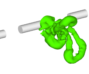
The DC geometry was devised to replicate the self-preserving structures of the far wake of the continuous circular cylinder, but in the near-wake region, which are commonly referred to as HSV or double roller (DR) vortices (Ferré & Giralt Reference Ferré and Giralt1989b; Vernet et al. Reference Vernet, Kopp, Ferré and Giralt1997). A well-established method to portray the shape of flow structures is to plot iso-surfaces with a certain level of pressure. Figure 4 shows pressure iso-surfaces obtained from an instantaneous field in the LES calculation of the DC wake. These plots clearly indicate the shape of the three-dimensional HSV and that the genesis of HSV is early in the wake, with their presence clearly observed by  $x/D \approx 3$ to
  $4$. This is distinct from the CC wake for which the three-dimensional rib structures take some time to develop (Hayakawa & Hussain Reference Hayakawa and Hussain1989). Figure 5 shows vector plots of velocity fluctuations in the
  $x$–
$x$– $y$ plane with
  $z=0$ for an instantaneous field obtained from PIV measurements in the DC wake. We will use the
  $u$,
$u$,  $v$ and
  $w$ symbols to denote the
  $x$-,
$x$-,  $y$- and
  $z$-velocity components, while an overbar on a quantity will denote its mean (time-averaged) value. In the near wake (
 $x/D < 10$), the rolls portrayed in figure 5(a) remind one of the typical patterns that are generated by the VKV in the CC wake, indicating that wake periodicity is maintained. Spectra of the streamwise velocity fluctuations (not shown for brevity) indicate that the Strouhal number is
  $S_{t} = 0.137$ in the DC wake, which is considerably lower than the corresponding values for the CC wake (
 $St=0.202$ from current LES at
  $Re=10^4$, in good agreement with the
  $St=0.202$ and
  $0.203$ values respectively reported by Norberg (Reference Norberg2003) and Dong et al. (Reference Dong, Karniadakis, Ekmekci and Rockwell2006) at similar
  $Re$). Figures 5(b) and 5(c) show that further downstream (
 $x/D > 30$), the intensity of these vortices in the
  $x$–
$x$– $y$ plane is still high and that the centres have been displaced considerably further from the centreline.

Figure 4. Iso-surfaces of  $(\hat {p}-p_{atm})/(\rho U_0^2)=-0.1346$ in the DC near wake at one instant of time from the LES simulation at
  $Re =1.0\times 10^4$. (a) Side view of
  $x$–
$x$– $y$ plane and (b) three-dimensional view of three different instantaneous vortices, labelled as HSV1, HSV2 and HSV3.

Figure 5. Vector plots of the instantaneous velocity fluctuations  $(u^\prime, v^\prime )$ in the
  $x$–
$x$– $y$ plane at
  $z=0$ (a) in the near (
 $3.5 \le z/D \le 7.5$), (b) middle–far (
 $29 \le z/D \le 35$) and (c) far (
 $68 \le z/D \le 76$) wakes of the DC. The vector scale used in (b) is 2.4 times larger than in (a). In each case, the arrow near the top of the figure frame denotes the length for the reference velocity,
  $U_0$. The data are from PIV measurements with model
  $M_2$ at a Reynolds number of
  $Re = 1.0 \times 10^4$ for panels (a,b), and with model
  $M_3$ at a Reynolds number of
  $Re = 4.0 \times 10^3$ for panel (c).
Figure 6 depicts instantaneous velocity fluctuation vectors, again obtained from PIV measurements, in  $x$–
$x$– $z$ planes at two different vertical levels. In this plane, the projection of the ‘legs’ of the HSV becomes apparent and illustrate why the HSV are also called double rollers. Relatively high strength rotation is observed around the HSV legs at a streamwise location as far downstream as
  $x/D=80$, as shown in figures 6(b) and 6(c). Consistent with the pressure contours in figure 4 and the velocity vectors in figure 6, figure 7 depicts the mean velocity vectors in the
  $y$–
$y$– $z$ plane at
  $x/D=10$ along with the iso-contours of the three mean vorticity components. In this figure, the alignment of the streamwise vorticity component with the DR pattern is clear. However, the
  $y$-vorticity is also aligned with the legs, while the
  $z$-vorticity can be seen further from the centreline. This mean flow pattern, with the periodic repetition of HSV, indicates the clear momentum exchange from the free stream in the gap region (i.e. between the solid cylinder segments) into the wake region. There are strong horizontal
  $z$-velocity components between the HSV near
  $y \approx 0$, which connects to the vertical momentum exchange associated with the head (or top) of the HSV (i.e. the
  $z$-vorticity, as seen in figures 5(a) and 7(a)). Figure 8 shows the mean streamwise vorticity along with the mean velocity vectors in
  $y$–
$y$– $z$ planes at
  $x/D = 20$ and
  $30$. The relatively strong mean cross-stream circulation in these plots indicates that this flow pattern remains for a remarkably long downstream distance. Thus, the footprint of the HSVs on the mean velocity field is a quite regular one, which impacts both the mean and fluctuating statistics of the flow. Further upstream, figures 9(a) and 9(b) show the centreline (
 $y=0$) profiles of the mean
  $z$- and
  $x$-velocity components, respectively, at several streamwise locations in the near wake (
 $x/D \le 10$). Figure 9(a) indicates that there are high values of the
  $z$-velocity moving fluid into the legs of the HSV that originates by
  $x/D=2$. Again, this points to the early formation of the HSV and the importance of the lateral entrainment as the HSV form. This lateral momentum transfer contributes to the relatively fast momentum recovery in the DC near wake, illustrated by the streamwise
  $x$-velocity component in figure 9(b) and which will be explored further in the next two subsections.

Figure 6. Vector plots of the instantaneous velocity fluctuations  $(u^\prime, w^\prime )$ in
  $x$–
$x$– $z$ planes (a) at
  $y/D=2$ in the middle (
 $11 \le z/D \le 17$), (b) at
  $y/D=3.7$ in the medium–far (
 $48 \le z/D \le 53$) and (c) at
  $y/D=5$ in the far (
 $77 \le z/D \le 83$) wakes of the DC. The arrow near the top of the figure frame denotes the length for the reference velocity,
  $U_0$. The data are from PIV measurements with model
  $M_2$ at a Reynolds number of
  $Re = 1.0\times 10^4$ for panels (a,b), and with model
  $M_3$ at a Reynolds number of
  $Re = 4.0\times 10^3$ for panel (c).

Figure 7. Mean velocity vectors and mean vorticity contours in the  $y$–
$y$– $z$ plane at
  $x/D=10$, obtained from the LES simulation: (a) spanwise vorticity component (
 $\overline {\tilde {\omega }}_z D/U_0$), (b) streamwise vorticity component (
 $\overline {\tilde {\omega }}_x D/U_0$) and (c) vertical vorticity component (
 $\overline {\tilde {\omega }}_y D/U_0$). In each case, the arrow near the top of the figure frame denotes the length for the reference velocity,
  $U_0$.

Figure 8. Mean velocity vector plots  $(\overline {\tilde {v}}, \overline {\tilde {w}})$ and mean vorticity contours (
 $\overline {\tilde {\omega }}_x D/U_0$) in the
  $y$–
$y$– $z$ plane at (a)
  $x/D=20$ and (b)
  $x/D=30$ from the LES simulation. In each case, the arrow near the top of the figure frame denotes the length for the reference velocity,
  $U_0$.

Figure 9. Profiles of (a) mean velocity  $\overline {\tilde {w}}/U_0$ and (b) mean velocity
  $\overline {\tilde {u}}/U_0$ components in the spanwise direction on the DC wake centreline (
 $y=0$) at several streamwise locations from the LES simulation.
3.2. Comparison of the continuous and DC near wakes
In this subsection we compare the CC near wake ( $x/D \le 10$) with the DC near wake using PIV measurements and LES results for
  $Re=1.0 \times 10^4$. The instantaneous data were ensemble averaged to determine the mean streamwise and transverse velocities, Reynolds shear stress and mean vorticity patterns on the measurement planes. Figure 10 shows the streamwise profiles of the mean streamwise velocity component (
 $\bar {u}$) on the flow centreline (
 $y=0$,
  $z=0$). Both simulations and measurements show that the recirculation length, i.e. the wake closure length (
 $L_{R}$), which is defined as the mean (time-averaged) closure point (i.e. the saddle point on the wake centreline,
  $y=0$), is much larger in the DC wake (
 $L_{R}/D=3.63$ from PIV measurements) than it is for the CC wake (
 $L_{R}/D =1.51$). Accordingly, the minimum value in the DC profile of figure 10 is much lower (more negative) than it is for the CC profile. It is observed that the CC profile recovers quite soon (
 $x/D \approx 3$) to a value as high as
  $\bar {u}/U_{0} \approx 0.70$, but there is a rapid slope change at
  $x/D \approx 3$ with much slower changes as the flow evolves downstream. In contrast, the momentum recovery is initially slower in the DC profile, but the rate of change (i.e. the slope of the curve) is much higher for the DC wake for
  $x/D > 3$. At
  $x/D=10$ both profiles have attained an almost identical level of
  $\bar {u}/U_{0} \approx 0.75$ at the
  $y=0$ centreline, although the slope remains higher for the DC wake at this point.

Figure 10. Comparison of mean streamwise velocity ( $\bar {u}/U_0$) on wake centreline (
 $y=0$) and mid-plane (
 $z=0$) for the DC and CC wakes. Lines show the LES results: DC wake (—), CC wake (– –). Symbols show the PIV results: DC wake
  $(\triangle )$, CC wake
  $(\circ )$.
As discussed in the previous subsection, the HSV are formed by  $x/D \approx 3$, with significant spanwise inflow by
  $x/D = 2$ such that the rate of change of the centreline velocity is likely related to the significant role of the HSV downstream of this point. In contrast, the VKV have emerged prior to
  $x/D = 1$. For example, Cantwell & Coles (Reference Cantwell and Coles1983) found a wake closure point of approximately
  $x/D = 1.2$, with the VKV formed by approximately
  $x/D \approx 0.7$. This relationship between the formation of a quasi-2-D vortex street and the wake closure point seems fairly consistent. The minimum in the streamwise velocity is closely related to the formation point of the vortices (see, e.g. the results of Taylor, Gurka & Kopp (Reference Taylor, Gurka and Kopp2014) for a range of 2-D bluff body shapes), with the vortices accelerating downstream, away from the formation point. For the CC, the inflow (entrainment) is dramatic in the range
  $1 < x/D < 3$, as indicated by the rapid increase in
  $\bar {u}/U_{0}$ in this range. In contrast, the HSV form further into the wake and do not have the same initial slope of
  $\bar {u}/U_{0}$. As pointed out above, the slope remains higher for the DC wake for an extended distance downstream with the
  $\bar {u}/U_{0}$ values becoming equal near
  $x/D=10$. Figure 11 shows the contours and selected vertical profiles of (
 $\bar {u}/U_{0}$) in the CC and DC wakes. Comparison of the contours in figures 11(a) and 11(b) confirms the differences in the length and intensity of the respective recirculation bubbles that were already inferred by figure 10. In addition, the contour plot for the DC wake in figure 11(b) reveals the comparatively high momentum deficit for the DC wake in the region behind the recirculation bubble. Inspection of the vertical
  $\bar {u}/U_{0}$ profiles in figure 11(c) together with the contour plots in figure 11(a,b) provides an indication of the different rates of flow development for these wakes. At the streamwise station,
  $x/D=2$, it is probably too early for the concept of wake width to make sense since the formation of the wake vortices is incomplete. However, at
  $x/D = 4$, the corresponding DC and CC profiles (figure 11d) suggest that the widths of both wakes are similar since the limiting
  $\bar {u}=U_{0}$ values are reached at
  $y/D \approx \pm 1.5$. Further downstream, by
  $x/D=8$ (figure 11e), the DC wake has become significantly wider. Note that the same effect can be observed in the contour plots of figure 11(a,b) when examining the isoline for
  $\bar {u}/U_{0}=1$. Figures 12(a) and 12(b) show the contours of the mean vertical component of velocity (
 $\bar {v}/U_0$) in the CC and DC wakes, respectively. The vertical
  $\bar {v}/U_0$ profiles at selected streamwise locations in figure 12(c–e) shows again the good agreement between the current PIV measurements and LES calculations. Figure 12(a) shows the presence of strongly negative
  $\bar {v}$ values in the near wake (
 $x/D \le 2$) of the CC wake, with a local minimum of
  $\bar {v}/U_0 = -0.29$ at
  $(x/D, y/D) \approx (1.34, 0.58)$. The presence of such foci of highly negative (or positive, in the
  $y < 0$ half-plane)
  $\bar {v}$ means that, on the average, fluid with higher momentum is driven inwards toward the midplane (
 $y = 0$) region, a mechanism that explains the fast momentum recovery of the CC near wake in figures 10 and 11(a), following the formation of the VKV, as discussed by Cantwell & Coles (Reference Cantwell and Coles1983), Ong & Wallace (Reference Ong and Wallace1996) and Ma, Karamanos & Karniadakis (Reference Ma, Karamanos and Karniadakis2000). In the corresponding
  $\bar {v}$ contours of the DC wake, figure 12(b), we see that the downwards (upwards for
  $y < 0$) flow pattern associated with the entrainment mechanism is considerably weaker and it occurs further downstream,
  $2 \le x/D \le 4$. Figure 12(b) also shows that this flow pattern in the DC wake is stronger closer to the cylinder,
  $x/D \le 2$, prior to the formation of the HVS. Another significant difference between the CC and DC contours of figures 12(a) and 12(b) is that, in the latter, there is a small but consistent flow pattern with fluid moving upwards in the upper half-wake in the
  $4 \le x/D \le 10$ streamwise region, a fact that is also reflected in the DC vertical profile of figure 12(e) (to be discussed later in § 4). This is associated with outward motions in the mid-plane of the HSV, as indicated in figures 5 and 6. Thus, the outward flow related to the vertical motions in the centre of HSV is more significant than the inward vertical motions, but the 3-D motions induced by the legs of the HSV are more important. Again, this contrasts with the near wake of the CC where the VKV vortices induce inward motions, which are strong initially, but decay rapidly as indicated by figure 12(c–e).

Figure 11. Vertical distribution of mean streamwise velocity ( $\bar {u}/U_0$) in the CC and DC wakes at
  $z=0$. Contours show LES results for (a) the CC wake and (b) the DC wake. Vertical profiles from the LES calculations for the DC (—) and CC (– –) wakes, along with the measured ones for the DC
  $(\triangle )$ and CC
  $(\circ )$ wakes at three downstream locations: (c)
  $x/D=2$, (d)
  $x/D=4$ and (e)
  $x/D=8$.

Figure 12. Vertical distribution of mean vertical velocity ( $\bar {v}/U_0$) in the CC and DC wakes at
  $z=0$. Contours show LES results for (a) the CC wake and (b) the DC wake. Vertical profiles from the LES calculations for the DC (—) and CC (– –) wakes, along with the measured ones for the DC
  $(\triangle )$ and CC
  $(\circ )$ wakes at three downstream locations: (c)
  $x/D=2$, (d)
  $x/D=4$ and (e)
  $x/D=8$.
The contours of the mean spanwise vorticity component,  $\overline {\omega }_z$, for the CC wake flow, shown in figure 13(a), confirm a strong average vortical activity in the CC near-wake region closest to the cylinder (
 $x/D\le 2$). Moreover, this plot also shows a horizontal strip with relatively low spanwise vorticity (
 $\overline {\omega }_z \le -0.2$), which is basically circumscribed within the midplane region,
  $|y/D| \le 1$. By comparison, the DC wake contours depicted in figure 13(b) show that large-scale vortices are similarly being generated behind the cylinder but instead of traveling close to the wake centreline they also move away from the horizontal midplane (see also figure 12b). Not surprisingly, figure 13(b) also shows highly negative
  $\overline {\omega }_z$ values in the
  $2 \le x/D \le 4$ streamwise region of the DC wake, that is, the region where strong downwards motion (figure 12b) was also observed. Note also in figure 13(b) that the region with significant spanwise vorticity levels (
 $\overline {\omega }_z\le -0.2$) reaches the
  $y/D=2$ edge of the plot at a streamwise location slightly below
  $x/D = 8$. This means that in the DC wake the large-scale vortices move away from the
  $y=0$ midplane as they travel downstream, as shown in figure 6. This is distinct to what is observed for the CC wake in figure 13(a). This evidence of fluid with significant vorticity and comparatively low momentum moving away from the midplane, hints again at the possibility of an enhanced growth rate of the DC wake (compared with the CC wake), a notion that will be analysed in detail below.

Figure 13. Vertical distribution of mean spanwise vorticity ( $\bar {\omega }_z D/U_0$) in the CC and DC wakes at
  $z=0$. Contours show LES results for (a) the CC wake and (b) the DC wake. Vertical profiles from the LES calculations for the DC (—) and CC (– –) wakes, along with the measured ones for the DC
  $(\triangle )$ and CC
  $(\circ )$ wakes at three downstream locations: (c)
  $x/D=2$, (d)
  $x/D=4$ and (e)
  $x/D=8$.
3.3. Wake growth characteristics
In this subsection the comparative analysis of the CC and DC wake flows is extended to the mid- and far-wake regions. Figure 14 shows the streamwise evolution of the maximum velocity defect,  $({\bar {u}}_d)_{max} = (U_0 - \bar {u})_{max}$, as measured in mid- and far-wake regions of the CC and DC wakes. The DC wake, as shown in figure 10, features high values in the base region, but further downstream, mean momentum in the DC wake recovers quickly. Figure 14 indicates that the enhanced mean momentum recovery in the DC wake persists in the mid-wake region with
  $10 \leq x/D \leq 20$. For example, at
  $x/D=16$ (i.e.
  $(x/D)^{-0.5} = 0.25$),
  $({\bar {u}}_d)_{max} = 0.19 U_0$ for the DC wake is clearly smaller than the corresponding value of
  $({\bar {u}}_d)_{max} = 0.23 U_0$ for the CC wake. Further downstream, we can see that the momentum recovery rates are similar in the two wakes, as indicated by the same slopes. However, the DC wake has a much smaller maximum momentum deficit at the same physical locations. As a result, the maximum velocity defect in the DC wake at
  $x/D=50$ is
  $({\bar {u}}_d)_{max} \approx 0.089 U_0$, which can be found at about
  $x/D=127$ in the CC wake; at just ten diameters further downstream in the DC wake (
 $x/D=60$) the equivalent streamwise location in the CC wake would be
  $x/D \approx 172$. Thus, even though the DC wake has a higher momentum deficit initially, it recovers much faster than the CC wake such that the maximum defect is significantly lower in the self-preserving far-wake region. A second quantity often used to characterize the growth rate of the CC wake is
  $y_{1/2}$, defined as the vertical location where the mean velocity is half of the maximum of
  $\overline {u}_d$. Figure 15 shows that in the near to mid wake of the DC, up to
  $x/D \approx 40$,
  $y_{1/2}$ rises much faster with downstream location than for the CC wake. In the streamwise region with
  $40 \leq x/D \leq 170$,
  $y_{1/2}$ increases at approximately the same rate in both wakes, i.e. both trendlines are parallel. For example, at
  $x/D = 50$ we have
  $y_{1/2} \approx 4.33 D$ in the DC wake whereas the equivalent streamwise location in the CC wake would be
  $x/D \approx 235$. Furthermore, a value of
  $y_{1/2} \approx 4.54 D$ for the DC wake at
  $x/D=60$ would be found at
  $x/D \approx 258$ in the CC wake.

Figure 14. Streamwise variation of the maximum mean velocity defect  $(\overline {u}_d/U_0)_{max}$ in the
  $x$–
$x$– $y$ vertical plane at
  $z=0$ in the CC and DC mid–far wake: (a)
  $2 \le x/D \le 25$; (b)
  $16 \le x/D \le 180$. All of the HWA and PIV measurements in the
  $70 \le x/D \le 180$ range were obtained with model
  $M_3$ at a Reynolds number of
  $Re=4.0\times 10^3$ (see tables 3 and 5). PIV measurements in the
  $10 \le x/D \le 56$ range were obtained at
  $Re=1.0\times 10^4$. Diaz et al.'s (Reference Diaz, Gavalda, Kawall, Keffer and Giralt1985) and Vernet's (Reference Vernet1999) results were obtained at
  $Re=9.0\times 10^3$ and
  $7.0\times 10^3$, respectively. The dashed and solid lines for the CC and DC data, respectively, indicate the
  $1/(x/D)^{0.5}$ variation associated with the self-preserving solution.

Figure 15. Variation of  $y_{1/2}/D$ with streamwise location in the CC and DC wake. All of the HWA and PIV measurements in the
  $70 \le x/D \le 180$ range were obtained with model M
 $_3$ at a Reynolds number of
  $Re=4.0\times 10^3$. PIV results in the
  $0 \le x/D \le 56$ range (both CC and DC) were obtained at
  $Re = 1.0\times 10^4$. Diaz et al.'s (Reference Diaz, Gavalda, Kawall, Keffer and Giralt1985) and Ferré & Giralt's (Reference Ferré and Giralt1989a) data were obtained at
  $Re = 9.0 \times 10^3$ whereas Vernet's (Reference Vernet1999) data were obtained at
  $Re = 7.0 \times 10^3$. The fitted equations of the self-preserving solutions for the CC wake (dashed line) and the DC wake (solid line) are
  $y_{1/2}/D=0.28((x/D)-3.05)^{0.5}$ and
  $y_{1/2}/D=0.40((x/D)+67.63)^{0.5}$, respectively.
Figure 15 depicts two distinct growth rates for the DC wake. For  $x/D \leq 56$ the spanwise periodicity of the HSVs, which are shed periodically from the DC, control the dynamics of the initial DC wake development. As the HSVs are advected downstream, the DC wake evolves towards a 2-D flow on the average since the HSVs are progressively randomized and their energy becomes indistinguishable from that of turbulence (as indicated by power spectra, not included here). These vortex structures lead to a significantly higher growth rate for the DC wake than for the CC wake, as discussed earlier. Beyond
  $x/D = 56$, the dynamics of the DC wake corresponds, on the average, to that of a CC, but with a virtual origin that is located far upstream of the physical origin. In fact, the position of this virtual origin so far upstream of the physical origin is an indicator of the enhanced entrainment and growth in the DC near wake since the growth rates of the DC and CC wakes are similar in the far wake (beyond
  $x/D = 56$).
It might be argued that quantities such as centreline  $\overline {u}_d$ and
  $y_{1/2}$, which were originally devised to characterize the growth rate of the CC wake, may not work well when applied to the analysis of the DC wake. In fact, the
  $\overline {u}_d$ vertical profiles for the DC wake in figure 16(a) show an unexpected feature with a local maximum at an intermediate vertical location, which is not present in the corresponding CC wake profiles (not shown here). Note that the local maximum in the
  ${\bar {u}}_d$ profile of figure 16(a) first appears at
  $x/D=16$. Similarly, an unexpected feature is also apparent in the
  $u_{RMS}$ vertical profiles shown in figure 16(b). In particular, the
  $u_{RMS}$ profiles early in the DC wake (
 $x/D \leq 26$) feature a local minimum in the vertical region with
  $0 \leq y/D \leq 2$, with two peaks, one on the centreline and the other off the centreline. As the wake grows, the
  $u_{RMS}$ peak values gradually decrease and at downstream station
  $x/D=170$, the profile is flatter, with low fluctuation levels, with maxima close to
  $y_{1/2}$.

Figure 16. Vertical profiles of (a) the mean streamwise velocity defect  $\overline {u}_d/U_0$ and (b) the root mean square streamwise velocity,
  $u_{RMS}/U_0$, at several streamwise stations in the
  $x$–
$x$– $y$ plane at
  $z=0$ in the DC wake for HWA measurements with the DC model,
  $M_3$, at a Reynolds number of
  $Re=4.0\times 10^3$.
In order to elucidate whether the fast rise of  $y_{1/2}$ for the DC wake in figure 15 is related to the vortical activity in the wake, we have plotted the vertical locations of maximum/peak values of
  $u_{RMS}$,
  $\overline {u^{\prime } v^{\prime }}$ and
  $\overline {\omega }_z$ at several streamwise locations in figure 17(a). Figure 17(a) shows that there is a good agreement between the vertical locations of the
  $\overline {\omega }_z$,
  $\overline {u^{\prime } v^{\prime }}$ and
  $u_{RMS}$ peaks suggesting that the peak locations in the mean field are indeed indicative of the periodic passage of coherent vortical structures. The similar plot for the CC wake is shown in figure 17(b). As expected, this plot confirms the well-known fact that in the CC wake the von Kármán vortices are moving away from the vertical midplane (
 $y=0$) as they travel downstream. However, comparison of figure 17(b) with 17(a) indicates that such a progressive vertical displacement of the vortical structures is much faster in the DC wake, which may be at least partially self-induced by the streamwise vorticity in the legs of the HSV, which are also stretched by the mean shear. For example, the VKV are located, on average, at approximately
  $y/D=\pm 1.6$ to
  $1.7$ at
  $x/D = 55$, which is smaller than the
  $y/D=\pm 4$ observed for the DC wake in figure 17(a) (noting that the latter vertical location is never reached in the CC wake for
  $x/D\le 180$). We have, therefore, seen that momentum recovery (figure 14), vertical spreading (figure 15) and upraising of vortical structures (figure 17) takes place much sooner in the DC wake than it does in the CC wake. Thus, it can be said that the downstream position where wake is considerably reduced (i.e.
  $\overline {u}_d$ approaches 0) occurs much earlier because of the segmentation of the cylinder, at which point the wake is much thicker.

Figure 17. Variation of the peak location in the  $y-$profiles of several flow variables for the (a) DC and (b) CC wakes. All of the data in this figure were obtained from PIV measurements. Measurements for
  $x/D \le 56$ were obtained with the model
  $M_2$ at
  $Re = 1.0\times 10^4$ whereas measurements for
  $x/D \ge 70$ were obtained with the model
  $M_3$ at
  $Re=4.0\times 10^3$. In (b) the experimental data previously reported by Diaz et al. (Reference Diaz, Gavalda, Kawall, Keffer and Giralt1985), obtained at
  $Re=9.0\times 10^3$, have been included.
Self-preservation analysis applied to the far wake of the continuous cylinder (Townsend Reference Townsend1956; Tang et al. Reference Tang, Antonia, Djenidi and Zhou2016) provides the following scaling laws for the centreline  $\overline {u}_d/U_0$ and
  $y_{1/2}/D$ quantities:
 \begin{gather} \frac{\overline{u}_d} {U_0} = C_1 \left[\frac{x-x_0}{D}\right]^{{-}0.5} \end{gather}
 \begin{gather}\frac{y_{1/2}} {D} = C_2 \left[ \frac{x-x_0}{D}\right]^{0.5}. \end{gather}
Considering that, as will be discussed further below, the vertical growth of the wake is closely related to the vertical displacement of vortical structures, it makes sense to use (3.2) to compare both wakes. For the CC far wake, values of  $C_2 \approx 0.20$ and
  $-x_0/D$ in the
  $25-125$ range have been reported in the literature (see Tang et al. (Reference Tang, Antonia, Djenidi and Zhou2016), and references therein). For the DC data in figure 15, we have
  $C_2 = 0.63$ and
  $x_0 = 1.9D$ in the region with
  $4 \leq x/D \leq 36$ and
  $C_2 = 0.40$ and
  $x_0 = -67D$ for
  $52 \leq x/D \leq 170$.
4. Scaling of wake growth and entrainment
We have seen that the difference between the DC and the CC wake is not at the conceptual level: in both cases, the notion of the wake being a region with low mean velocity and high vorticity fluctuation levels holds. The difference between the two wakes is not in their turbulence intensity: the velocity and vorticity fluctuation levels (in the  $z=0$ plane) in the DC and the CC wakes are of the same order of magnitude. The reason for the different wake growth rates between both wakes is due to the significant changes in the large-scale vortices induced in the near wake by the discontinuity in the cylinder geometry. In the DC near wake, the flow is three-dimensional
  $(\overline {\tilde {w}}/U_0 \neq 0)$ and dominated by the shed HSV and the strong shear-aligned vorticity in their legs. In the CC, the mean flow is initially almost two-dimensional
  $(\overline {\tilde {w}}/U_0 = 0)$ and controlled by the spanwise vorticity of the shed Kármán vortices with also the weaker vorticity associated with the ribs or legs of incipient hairpin vortices. A complete analogy between both wakes, on an average flow basis, would only hold when
  $z$-velocities are close to zero in the DC wake (
 $\overline {\tilde {w}}(x, y, z)/U_0 \approx 0$), a situation only possible at large downstream distances. Notwithstanding, it should be noted that the dynamics of HSV in the DC wake will help to understand their role in wake growth and entrainment in both wake flows.
Let us consider a simple scaling analysis to illustrate the effects on the three-dimensional mean flow associated with the shedding of HSV in the DC wake. The (mean) mass conservation requirement on a small control volume around the mid-span centreline, ( $x,0, 0$) is
 \begin{equation} \frac{{\partial} \overline{\tilde{u}}}{{\partial} x} (x,0,0) ={-} \frac{{\partial} \overline{\tilde{w}}}{{\partial} z} (x,0,0)-\frac{{\partial} \overline{\tilde{v}}}{{\partial} y} (x,0,0) .\end{equation}
If we consider that  $ {\partial } \overline {\tilde {w}}/ {\partial } z \approx {\rm \Delta} w / L$,
  ${\rm \Delta} w$ can be estimated as the total drop (from peak to peak) measured in a centreline
  $z$-profile (see figure 9a), and assume that the scaling
  $(\overline {u}_d /U_0) \approx (x/D)^{-0.5}$ (see § 3.3 and figure 14a) is approximately valid in the near DC wake, then (4.1) becomes
 \begin{equation} \frac{{\partial} \overline{\tilde{u}}}{{\partial} x} (x,0,0) ={-} \frac{{\partial} \overline{\tilde{u}}_d}{{\partial} x} (x,0,0) \approx \frac{1}{2} \left( \frac{U_0}{D} \right) \left( \frac{x}{D}\right)^{{-}1.5} \approx \frac{{\rm \Delta} w(x)}{L}-\frac{{\partial} \overline{\tilde{v}}}{{\partial} y} (x,0,0) .\end{equation}
If we assume that the inflow in the  $y$-direction and toward the midplane (
 $x,0,0$) that is induced at the front of each HSV by its top rotation, is approximately balanced by the outflow in the opposite
  $y$-direction and toward the external flow that occurs at the back of each HSV, then
  $ {\partial } \overline {\tilde {v}}/ {\partial } y \approx 0$ or smaller than
  $ {\partial } \overline {\tilde {w}}/ {\partial } z$ in absolute terms. If this is the case,
  $ {\partial } \overline {\tilde {u}}/ {\partial } x \approx - {\partial } \overline {\tilde {w}}/ {\partial } z$, and all
  $\overline {\tilde {w}}$ profiles should scale as
  $(\overline {\tilde {w}}/U_0) (x/D)^{1.5}$.
Figure 18 depicts the centreline ( $y=0$)
  $z$-profiles of the dimensionless spanwise velocity
  $(\overline {\tilde {w}}/U_0) (x/D)^{1.5}$ at several streamwise locations. The profiles in this figure show that the proposed scaling for
  $\overline {\tilde {w}}$ holds in the DC wake for
  $x/D \le 30$ in the spanwise direction. These results also show that the lateral fluid exchange mechanism and momentum transfer in the spanwise direction associated with the HSV, contribute significantly to the asymptotic increase with
  $x/D$ of the average centreline velocity
  $\overline {\tilde {u}}(x, 0, z)$ toward
  $U_{0}$. It should be noted that, as HSV are advected downstream and their spanwise and vertical locations progressively randomized by turbulence, and as the mean spanwise velocity tends to zero,
  $\overline {\tilde {w}} \approx 0$, the role of
  $ {\partial } \overline {\tilde {v}}/{ {\partial } y}$ in DC wake growth and entrainment progressively becomes predominant. Simultaneously, the dominant contribution of the HSV to the total kinetic energy of the DC wake flow should also progressively diminish. The power spectral density of the streamwise velocity fluctuations, not shown here, indicates that this occurs for
  $x/D \ge 120$.

Figure 18. Selected spanwise profiles of normalized mean  $z$-velocity,
  $(\overline {\tilde {w}}/U_0) (x/D)^{1.5}$, at the centreline (
 $y=0$) and several streamwise locations in the DC wake, as indicated in the legend, from LES simulations.
The implications of the above scaling analysis (figure 18) in the early DC wake development and growth by the large-scale motions that are linked to the progressive stretching of HSV, can only be fully understood when analysing the streamwise evolution of  $\overline {\tilde {v}}$ profiles in the transverse direction at
  $z/D=3.75$ and
  $0$. Figure 19(a) shows that the transverse
  $\overline {\tilde {v}}$ profiles at the middle of the gap between cylinder segments (
 $z/D=3.75$) tend towards self-similarity as
  $x/D$ increases, when scaled as
  $(\overline {\tilde {v}}/U_0) (x/D)^{0.5}$. According to (4.2), this can only be the case if
  $\overline {\tilde {w}}=0$ and
  $ {\partial } \overline {\tilde {w}}/{ {\partial } z}=0$, as is the case in figure 18, and the streamwise variations of
  $\overline {\tilde {u}}$ and
  $\overline {\tilde {v}}$ are solely caused by a net vertical inflow of fluid from the external, at both sides of the wake, towards the centre plane. Since this is also the case for a fully developed CC wake, it justifies the current adoption of the scaling arising from the self-preservation analysis of the CC far wake (Tang et al. Reference Tang, Antonia, Djenidi and Zhou2016), where (
 $\overline {\tilde {v}}/U_0) \propto (x/D)^{-0.5}$, with distances normalized with
  $y_{1/2}$. Results in figure 19(a) are consistent with the mean vertical motions portrayed in figure 8.

Figure 19. Selected vertical profiles of the normalized mean  $y$-velocity,
  $(\overline {\tilde {v}}/U_0) (x/D)^{0.5}$, at several streamwise locations in the DC wake at (a) the mid-gap spanwise location (
 $z/D=3.75$) and (b) the mid-segment spanwise location (
 $z=0$), from the LES simulations.
The vertical  $\overline {\tilde {v}}$ profiles at the mid-segment (
 $z=0$) spanwise locations shown in figure 19(b) also scale well with
  $(\overline {\tilde {v}}/U_0) (x/D)^{0.5}$ for
  $x/D \le 30$. At this spanwise location at the centre of the HSV (
 $z/D=0$) the vertical fluid motion has to be outward, with
  $ {\partial } \overline {\tilde {v}}(x,0,0)/ {\partial } y > 0$, and opposite to that in figure 19(a) for
  $z/D=3.75$, because HSV protrude vertically into the external flow to drive wake growth while stretched by the strain field, as reported by Kopp et al. (Reference Kopp, Giralt and Keffer2002) for a fully developed CC turbulent wake. In this CC case, HSV were located inside turbulent bulges that protruded into the external flow and defined the intermittent turbulent/non-turbulent wake interface.
Let us assume that such a scale for the mean vertical motion in the DC wake, say  $V_\omega$, is also proportional to the rate of vertical growth of the wake. Then if
  $\delta (x_{0})$ is the thickness of the DC wake at a reference streamwise location
  $x_{0}$, we can infer the following scaling for the wake rate of growth,
 \begin{equation} \delta(x)-\delta(x_0) \approx V_{\omega} \triangle t \propto U_0 \left( \frac{x}{D} \right)^{{-}0.5} \left( \frac{x-x_0}{U_0} \right) \propto \left( x^{0.5} D^{{-}0.5} \right), \end{equation}
or, equivalently, a wake vertical growth according to  $\triangle \delta (x)/D \propto (x/D)^{0.5}$. Note the consistency of this result with the
  $y_{1/2}/D \propto (x/D)^{0.5}$ behaviour observed in subsection 3.3 for the DC near-to-mid wake (see figure 15). The outward vertical motion of the HSV shown in figure 19(b), together with the increase in the centreline streamwise velocity as
  $x/D$ increases, has to fulfil continuity and be matched by the vertical inward fluid motion of figure 19(b), coupled with the spanwise motion towards the centre of the HSV (
 $ {\partial } \overline {\tilde {w}}/ {\partial } z \ll 0$), as illustrated in figure 18 and discussed in detail below.
Figures 19(a) and 19(b) show, on a comparable ordinate scale, the evolution of the initial growth of the DC wake in terms of the transverse velocity at the spanwise side and at the centre of the HSV, respectively. These streamwise evolutions of dimensionless vertical velocities, which are clearly related to momentum transfer into the wake from the external flow and to wake growth by HSV stretching, respectively, are dominated by the shedding of HSVs. These two figures show that both inward and outward transverse profiles progressively evolve towards self-similar profiles at both spanwise locations as  $x/D$ increases. Figure 19(a) shows that at
  $z/D=3.75$ the recirculation associated with the shed HSV causes a reverse flow inward at the sides of each HSV, which is linked to the upward flow observed at their centre (
 $z/D=0$) in figure 19(b). This recirculation pattern, which also involves the spanwise velocity component of figure 18, is initially dominated by the kinking of the shed HSVs caused by the flow from the gap between cylinder segments toward the back of each cylinder centre. As a result, the highest vertical velocities occur at the centre of the HSV for
  $x/D < 10$, as observed in figure 19(b). Further downstream, as
  $x/D$ increases, vertical velocities and the wake growth shown in figures 14 and 15, become more and more controlled by the stretching of the HSV. This alignment and stretching by the strain field, makes the HSV to protrude toward the external flow, with vertical velocities progressively showing a self-similar behaviour for
  $x/D \ge 26$ in figure 19(b). Thus, all vertical motions clearly associated with the HSV in the DC wake show self-similarity in figures 19(a) and 19(b) when scaled according to CC wake velocity and length reference parameters. This is also the case for the gradients of the vertical profiles at the centre of the HSV in figure 19(b), where
  $ {\partial } \overline {\tilde {v}}/ {\partial } y (x,0,0) \propto (U_{0}/D)(x)^{-1.6}$ for
  $x/D \le 30$, which is very close to the
  $-$1.5 power variation that holds for fully developed turbulent CC wakes. Thus, the average fluid motions that are related wake growth and entrainment by the HSV in the DC near wake scale as in the CC wake, where large-scale structures like the current HSV have been identified and claimed to play a dominant role in wake growth and entrainment.
The smooth and self-equilibrating evolution towards self-similarity and self-preservation in the DC wake flow shown in figure 19, which is controlled by shed HSV, from genesis to self-preservation, is consistent with the streamwise variations of the maximum mean velocity-defect and of  $y_{1/2}/D$ shown in figures 14 and 15, respectively, for the DC wake. The same behaviour towards self-similarly and wake growth mechanism associated with donut-like vortices or DRs was also reported by Vernet et al. (Reference Vernet, Kopp, Ferré and Giralt1999) and Kopp et al. (Reference Kopp, Giralt and Keffer2002), respectively, in CC turbulent wakes, but for much larger streamwise distances. In the CC case, the large-scale coherent motions that develop from the hairpin vortices arising from instabilities in the VKV street (Cao et al. Reference Cao, Chen, Zhou, Antonia and Zhou2014; McClure et al. Reference McClure, Pavan and Yarusevych2019), require much larger advection times or streamwise distances to develop and become shear aligned, i.e.
  $ {\partial } \overline {\tilde {v}}/ {\partial } y (x,0,0) \propto (U_{0}/D)(x)^{-1.5}$. The vertical profiles at the mid-gap (
 $z/D=3.75$) and mid-segment (
 $z=0$) spanwise locations, shown in figure 19, together with the scaling of (4.3), confirm that the DC geometry brings into the near wake, not only the HSV, but also another characteristic feature of the far CC wake, i.e. the self-preservation of the mean velocity profiles.
The incorporation of high momentum free-stream fluid by the linked lateral–vertical entrainment process, depicted in figures 8 and 5(b,c), which is governed by HSV, implies the extraction of energy from the mean flow and the persistence of turbulence in the wake. Mean shear production contours calculated from PIV data measured in the DC, not shown here, indicate that the highest production rates occur at  $y_{1/2}$ and at the centre of the HSV for
  $x/D \ge 5$. This is consistent with the momentum transfer associated with the donut-like structures reported by Vernet et al. (Reference Vernet, Kopp, Ferré and Giralt1999) in a CC wake at
  $x/D=150$, and with the role in the entrainment process that has been claimed for the DR identified in the far wake of a CC by Kopp et al. (Reference Kopp, Giralt and Keffer2002). When this entrainment process is completely established in the wake of the DC at approximately
  $x/D=50$, i.e. when the wake grows with
  $(x/D)^{0.5}$, as shown in figure 15, and
  $ {\partial } \overline {\tilde {v}}/ {\partial } y (x,0,0) \propto (U_{0}/D)(x)^{-1.5}$, HSV should be shear aligned, optimally stretched, and scalable according to (4.2) and figure 19. The CC wake also grows with
  $(x/D)^{0.5}$, as shown in figure 15. Note that turbulent bulges and the corresponding large-scale motions or DR in both the DC and CC wakes (Kopp et al. Reference Kopp, Giralt and Keffer2002) are in a region where high momentum free stream fluid can be entrained, as shown for the DC in figures 5, 6, 7 and 8. Current findings also confirm that the entrainment process is the result of linked lateral rotating motions and vertical outward jet-like motions and the rear of the DR. The overall process is strongly dominated by the stretching of the shear aligned vortex legs, i.e. by lateral entraining motions and inward motions at the front of the HSV, that in turn generate the outward jet-like motions responsible for wake growth. Turbulent diffusion seems to play a secondary role in the entrainment process but necessary one in the energy cascade and dissipative nature of the turbulent wake flow.
5. Conclusions
A study of the existing literature indicates that there is a lack of agreement regarding the mechanism of entrainment, with various studies finding differences in the relative importance of the nibbling and engulfment mechanisms. This suggests a significant flow dependence and that by controlling the development of the large-scale structures, one can control the extent to which each of these mechanisms contribute to the overall entrainment rate. The hypothesis motivating this study is that enhancing vortices that are in alignment with the mean shear will increase the rate of entrainment based on observations of flow structure and entrainment in the self-preserving regions of far wakes. We test this hypothesis by modifying the formation of the vortices in the near wake of a circular cylinder such that shear-aligned HSV are formed early in the wake. We contrast this with growth and spread of the circular cylinder wake, which is controlled by the von Kármán vortex street in the near wake. To achieve this, we develop and examine what we call a DC wake.
The turbulent flow in the wake of the DC was investigated both experimentally and numerically to ascertain the nature of the large-scale flow patterns and how these alter the overall growth and spread of the wake. The dominant flow structures in the DC wake are shown to be quasi-periodic, 3-D HSV, which are fully formed by about  $x/D \approx 3$. This structure contrasts with the periodic quasi-2-D VKV in the near wake of the CC. Following the vortex formation region of both wakes, the DC wake grows at a much more rapid rate than the CC wake, although the rate of initial development of the quasi-2-D Kármán vortices is significantly higher within
  $x/D < \approx 3$. However, the Kármán vortices decay quickly because of the lack of shear alignment and the HSV then develop a high rate over a significantly longer spanwise distance. So, while the wakes are about the same thickness at
  $x/D=4$, the DC wake is substantially thicker by
  $x/D \approx 8$ and maintains a higher growth rate until approximately
  $x/D \approx 50$. Further downstream, beyond
  $x/D \approx 50$, the wakes grow at the same rates, consistent with the 2-D self-preserving solution. However, the DC wake is significantly thicker, such that, at
  $x/D = 50$, the mean velocity half-width almost 3 times larger than that for the CC at the same physical location. At this same point, the maximum velocity defect for the DC is approximately half that for the CC even though the maximum velocity defect is significantly greater in the cylinder base region. All of this indicates a much greater entrainment rate for the DC with fully formed HSV in the near-wake region. The results indicate that the DC wake has a self-preserving form in the near wake region, but with a rate that is higher than in the fully developed far wake region. A simple scaling analysis indicates that the lateral entraining motions and the vertical stretching of the HSV can explain the growth rate of the wake.
The current findings have several implications beyond the possible development of engineering tools to increase (or suppress) turbulent mixing rates. First, with respect to self-preserving flows, it is well known that the virtual origin of self-preserving plane turbulent wakes is variable for different bluff bodies or for similar bluff bodies but in different laboratory settings. The implication from the current work is that enhancing shear-aligned vorticity in the initial conditions should decrease the position of the virtual origin, i.e. enhancing wake thickness and reducing the velocity defect. Modifying the values of  $L/D$ and
  $S/D$ for the DC would do this, as could other geometric (including variable cylinder diameters along the span) or flow discontinuities for circular cylinders. Second, for other turbulent shear flows, enhancing shear-aligned vorticity should have similar effects. This would include plane turbulent jets and plane mixing layers, which, like plane turbulent wakes, tend to have primary instabilities which induce the formation of vortices that are orthogonal to the mean shear. This could also include the effects of trips for the transition of turbulent boundary layers. However, examination of such details remains for future work.
Declaration of interests
The authors report no conflict of interest.


