


1 Introduction
The interaction between vortices and the surfaces of solid structures is a ubiquitous feature of bluff-body flows and high-angle-of-attack aerodynamics associated with a broad range of aerospace structures, including manoeuvring and flapping wings, blades on helicopter rotors and gas turbine engines, the aerodynamic forebodies of missiles and high-performance aircraft, delta wings, strakes and leading-edge extensions (Ol & Gharib Reference Ol and Gharib2003; Bridges Reference Bridges2010; Mulleners, Kindler & Raffel Reference Mulleners, Kindler and Raffel2012; Yilmaz & Rockwell Reference Yilmaz and Rockwell2012). The strength, internal structure and evolution of these vortices has a significant impact on aerodynamic loads (Leishmann & Beddoes Reference Leishmann and Beddoes1989; Shyy et al. Reference Shyy, Lian, Tang, Liu, Trizila, Stanford, Bernal, Cesnik, Friedmann and Ifju2008; Eldredge, Wang & Ol Reference Eldredge, Wang and Ol2009; Cleaver, Wang & Gursul Reference Cleaver, Wang and Gursul2013). Also, the evolution of the leading-edge vortex (LEV) on periodically oscillating wings has been shown to be a dominant influence on the structure of unsteady wakes (Lewin & Haj-Hariri Reference Lewin and Haj-Hariri2003; Lua et al. Reference Lua, Lim, Yeo and Oo2007; Eslam Panah & Buchholz Reference Eslam Panah and Buchholz2014).
Because of the importance of these structures, studies of vortex kinematics have been performed for a broad range of airfoil motions and geometries (Koochesfahani Reference Koochesfahani1989; Triantafyllou, Triantafyllou & Gopalkrishnan Reference Triantafyllou, Triantafyllou and Gopalkrishnan1991; Triantafyllou, Triantafyllou & Grosenbaugh Reference Triantafyllou, Triantafyllou and Grosenbaugh1993; Anderson et al. Reference Anderson, Streitlien, Barrett and Triantafyllou1998; Lai & Platzer Reference Lai and Platzer1999; Lewin & Haj-Hariri Reference Lewin and Haj-Hariri2003; Lua et al. Reference Lua, Lim, Yeo and Oo2007; Kang et al. Reference Kang, Aono, Cesnik and Shyy2011; Choi, Colonius & Williams Reference Choi, Colonius and Williams2015). In hovering flight, the LEV has been observed to be approximately stationary over the suction surface of the wing, thereby allowing for the production of higher lift coefficients (Ellington et al. Reference Ellington, van den Berg, Willmott and Thomas1996; Bomphrey et al. Reference Bomphrey, Lawson, Harding, Taylor and Thomas2005; Muijres et al. Reference Muijres, Johansson, Barfield, Wolf, Spedding and Hedenstrom2008; Warrick, Tobalske & Powers Reference Warrick, Tobalske and Powers2009). Pitt Ford & Babinsky (Reference Pitt Ford and Babinsky2013) deduced that essentially all of the bound circulation on an airfoil in a starting translational motion could be attributed to the LEV, and Wojcik & Buchholz (Reference Wojcik and Buchholz2014a ) demonstrated that the circulation contained within the LEV on a rotating flat plate at high angle of attack could significantly exceed the bound circulation predicted locally by thin airfoil theory at the same angle of attack and approaching flow velocity (assuming validity of the theory under these conditions).
Recently, several studies have focused on the means by which flow three-dimensionality can delay the detachment of the LEV. Citing the core-wise flow observed within the LEVs of delta wings, Ellington et al. (Reference Ellington, van den Berg, Willmott and Thomas1996) proposed spanwise flow as being necessary for the perpetual attachment of LEVs often observed on rotating wings, as the resulting centrifugal pumping can provide a means of balancing the shear-layer flux of vorticity into the LEV. However, subsequent studies have found that rotation does not necessarily produce a significant spanwise flux of vorticity (Birch & Dickinson Reference Birch and Dickinson2001; Carr, Chen & Ringuette Reference Carr, Chen and Ringuette2012). Lim et al. (Reference Lim, Teo, Lua and Yeo2009) showed that vortex stretching could delay detachment of the vortex, while other studies (Shyy et al. Reference Shyy, Trizilla, Kang and Aono2009; Taira & Colonius Reference Taira and Colonius2009; Carr et al. Reference Carr, Chen and Ringuette2012; Jantzen et al. Reference Jantzen, Taira, Granlund and Ol2014) proposed that the downwash induced by the tip vortex plays a role in anchoring the LEV to the leading edge. Similarly, Beem, Rival & Triantafyllou (Reference Beem, Rival and Triantafyllou2012) and Wong, Kriegseis & Rival (Reference Wong, Kriegseis and Rival2013) showed that spanwise flow had no effect on either the circulation of the LEV nor the force history on a swept wing of large aspect ratio.
On the other hand, the diffusive flux of secondary vorticity from the surface must also be considered in order to fully understand vortex development. While there are many noteworthy examples within the literature wherein the diffusive flux of vorticity from the surface of an airfoil has been shown to correlate directly with important events in the flow (Visbal & Shang Reference Visbal and Shang1989; Acharya & Metwally Reference Acharya and Metwally1992; Shih & Ho Reference Shih and Ho1994; Kuo & Hsieh Reference Kuo and Hsieh2001; Eslam Panah, Akkala & Buchholz Reference Eslam Panah, Akkala and Buchholz2015), Shih & Ho (Reference Shih and Ho1994) were among the first to definitively conclude that the vortex–airfoil interaction has a significant impact on the development of the LEV. Specifically, their analysis revealed diffusive effects to be of the same order of magnitude as convective effects during the formation of the LEV. However, the literature contains relatively little discussion about how the vortex–airfoil interaction, and resulting diffusive flux of vorticity from the surface, affects the growth and evolution of the LEV. A more thorough characterization of the fundamental physics is therefore needed before effective flow control techniques can be developed (Acharya & Metwally Reference Acharya and Metwally1992).
It is well established that the diffusive flux resulting from the interaction between a forming vortex and the surface will result in the accumulation of secondary vorticity of the opposite sign to the primary vortex. Acharya & Metwally (Reference Acharya and Metwally1992) further hypothesized that the accumulation of this secondary vorticity near the leading edge is concomitant with the detachment of the LEV from the leading-edge shear layer. In their study of a pitching NACA 0012 airfoil, they also found great success in characterizing the dynamic stall process based on the transient behaviour of critical features within the surface pressure distributions. Visbal & Shang (Reference Visbal and Shang1989) computed the vorticity flux from the surface of a pitching airfoil and showed that the net flux was only non-negligible during the period of angular acceleration. However, after the acceleration phase, they found significant spatially distinct sources of positive and negative vorticity on the surface, which could be expected to affect the local vorticity dynamics.
The secondary vorticity flux undoubtedly leads to a weakening of the primary vortex through its entrainment and resulting cross-cancellation. For example, significant weakening of the LEV was observed by Visbal (Reference Visbal2009), as a result of secondary vorticity entrainment into the leading-edge vortex on a nominally two-dimensional plunging airfoil when the flow was transitional. Wojcik & Buchholz (Reference Wojcik and Buchholz2014b ) analysed the transport of vorticity on a rotating wing, and inferred from their results that the annihilation of primary LEV vorticity via the entrainment and cross-cancellation of secondary vorticity was the primary mechanism balancing the influx of leading-edge shear-layer vorticity. They noted that, while the work did not show cross-cancellation alone to be a sufficient condition for vortex stability, it may be a necessary condition, as it was demonstrated to limit LEV circulation. Subsequently, Eslam Panah et al. (Reference Eslam Panah, Akkala and Buchholz2015) obtained quantitative measurements of the diffusive vorticity flux, observing its effect on LEV development for a two-dimensional airfoil and demonstrating the robustness of the phenomenon for pure translational motions. Their analyses showed that approximately half of the vorticity that was introduced into the LEV through the leading-edge shear layer could be lost through cross-cancellation.
The primary goal of this paper is to provide a rigorous characterization of the formation and evolution of the leading-edge vortex formed on plunging wings considering both the convective transport of vorticity in the bulk flow as well as the diffusive transport from the surface. The nominally two-dimensional flow produced by a high-aspect-ratio flat-plate airfoil undergoing a pure-plunge motion is first considered. Once this baseline flow is understood, a finite-aspect-ratio plate is considered, which will introduce significant three-dimensional convective vorticity transport mechanisms into the flow. This secondary case will be used to both support a proposed new mechanism by which the surface diffusive flux of vorticity governs the evolution of the LEV, and to demonstrate how it can be mitigated by three-dimensional effects to delay detachment and potentially enhance lift. In contrast to some of the aforementioned observations of stable vortices on rotating wings, this study will focus on the growth and evolution of vortices formed on surfaces in linear plunge motions. The revealed physical mechanisms, by which the diffusive flux serves to destabilize the LEV, will provide a foundation to inform future strategies for active or passive control of vortex evolution and aerodynamic loads, as we not only identify and describe the fundamental transport behaviour by which this process occurs, but also use this insight to specifically characterize how the vorticity budget of the LEV must be altered in order to achieve stability.
2 Methods
Experiments were conducted in a closed-return water channel to investigate vortex generation and evolution on two plunging aerodynamic bodies: a flat-plate airfoil (aspect ratio 4, spanning the height of the water channel) and a rectangular wing of aspect ratio 2. The two cases will be denoted as the AR4 and the AR2 cases, respectively. The airfoil and wing were constructed out of aluminium, and both had a chord length
 $c$
of 76.2 mm, thickness of 3.2 mm and leading and trailing edges that were rounded with a constant radius of half the plate thickness. A schematic of the cross-sectional profile of the two plates is given in figure 1(a), with each of the planform profiles shown in figure 1(b). Figure 1(b) also illustrates the chordwise arrays of pressure taps that were located on the surface of the two plates, the spanwise positions of which serve to identify the four planes considered in this study. The positions of each of these pressure taps are reported in § 2.2. Figure 1(b,c) also illustrates the stainless steel bracket assemblies used to rigidly support the plates, which consist of a 7.9 mm diameter rod with a 17.5 mm diameter custom cylindrical coupling which attached to a precision-machined clamp that supported the full chord length of the plate. It should be noted that all spanwise dimensions are measured from the root of the plate and not from the top of the clamp assembly, which figure 1(c) shows extending 7.9 mm above the root of the plate.
$c$
of 76.2 mm, thickness of 3.2 mm and leading and trailing edges that were rounded with a constant radius of half the plate thickness. A schematic of the cross-sectional profile of the two plates is given in figure 1(a), with each of the planform profiles shown in figure 1(b). Figure 1(b) also illustrates the chordwise arrays of pressure taps that were located on the surface of the two plates, the spanwise positions of which serve to identify the four planes considered in this study. The positions of each of these pressure taps are reported in § 2.2. Figure 1(b,c) also illustrates the stainless steel bracket assemblies used to rigidly support the plates, which consist of a 7.9 mm diameter rod with a 17.5 mm diameter custom cylindrical coupling which attached to a precision-machined clamp that supported the full chord length of the plate. It should be noted that all spanwise dimensions are measured from the root of the plate and not from the top of the clamp assembly, which figure 1(c) shows extending 7.9 mm above the root of the plate.

Figure 1. (a) Cross-sectional and (b) planform geometries of the flat plates. (c) Mounting bracket used to secure the plates.
The plunge motion was articulated using a scotch yoke mechanism that was driven by an Emerson Control Techniques XVM-6011-TONS motor and an Emerson EP-B amplifier. The plate chords were aligned with the flow direction and driven to oscillate transversely in a sinusoidal motion with displacement specified as:
 $$\begin{eqnarray}h(t)=-h_{0}\sin (2\unicode[STIX]{x03C0}ft).\end{eqnarray}$$
In the present study, we consider a plunge amplitude of
 $h_{0}/c=0.3$
with reduced frequency
$h_{0}/c=0.3$
with reduced frequency
 $k=\unicode[STIX]{x03C0}fc/U=1.57$
, corresponding to a Strouhal number
$k=\unicode[STIX]{x03C0}fc/U=1.57$
, corresponding to a Strouhal number
 $St=2fh_{0}/U=0.3$
, where
$St=2fh_{0}/U=0.3$
, where
 $h_{0}$
and
$h_{0}$
and
 $f$
are the plunge amplitude and oscillation frequency from (2.1),
$f$
are the plunge amplitude and oscillation frequency from (2.1),
 $c$
is the chord length and
$c$
is the chord length and
 $U$
is the free-stream velocity. These parameters describe the kinematics of one of the plunging airfoil cases examined by Eslam Panah et al. (Reference Eslam Panah, Akkala and Buchholz2015), and are broadly representative of the parameters describing animal flight and swimming (Triantafyllou et al.
Reference Triantafyllou, Triantafyllou and Gopalkrishnan1991, Reference Triantafyllou, Triantafyllou and Grosenbaugh1993; Taylor, Nudds & Thomas Reference Taylor, Nudds and Thomas2003).
$U$
is the free-stream velocity. These parameters describe the kinematics of one of the plunging airfoil cases examined by Eslam Panah et al. (Reference Eslam Panah, Akkala and Buchholz2015), and are broadly representative of the parameters describing animal flight and swimming (Triantafyllou et al.
Reference Triantafyllou, Triantafyllou and Gopalkrishnan1991, Reference Triantafyllou, Triantafyllou and Grosenbaugh1993; Taylor, Nudds & Thomas Reference Taylor, Nudds and Thomas2003).
Experiments were conducted in a free-surface water channel with test section width of 0.61 m and water depth of 0.31 m. The free surface was constrained 0.6 m upstream and downstream of the airfoil or wing by a rigid surface plate as illustrated in figure 2. In order to reduce the effects of root boundary conditions, the underside of the free-surface plate was located less than 1 mm above the clamp assembly shown in figure 1(c). Similarly, the gap between the tip of the AR4 airfoil and the bed of the water channel was also less than 1 mm. The water channel has flow conditioning consisting of an 8:1 contraction ratio, honeycomb and five screens to maintain free-stream turbulence intensity below 0.3 %. Free-stream velocity is held constant for all experiments, producing a chord-based Reynolds number of
 $Re_{C}=10\,000$
.
$Re_{C}=10\,000$
.

Figure 2. Imaging configuration for stereo PIV measurements.
2.1 Vorticity transport analysis
The evolution of the leading-edge vortex was quantified by constructing a circulation budget comprised of sources and sinks based on the mechanisms of vorticity transport within a chordwise planar control region enclosing the vortex. The control region is shown schematically in figure 3. The control region defined in this way does not specifically isolate the LEV, but allows the creation of a circulation budget that takes into account all sources of vorticity that have an impact on the development of the LEV. The budget governing the rate of change of circulation within the control region is given by Eslam Panah et al. (Reference Eslam Panah, Akkala and Buchholz2015):
 $$\begin{eqnarray}\frac{\text{d}\unicode[STIX]{x1D6E4}_{z}}{\text{d}t}=-\int _{A_{z}}u_{z}\frac{\unicode[STIX]{x2202}\unicode[STIX]{x1D714}_{z}}{\unicode[STIX]{x2202}z}\,\text{d}A_{z}+\int _{A_{z}}\left(\unicode[STIX]{x1D714}_{x}\frac{\unicode[STIX]{x2202}u_{z}}{\unicode[STIX]{x2202}x}+\unicode[STIX]{x1D714}_{y}\frac{\unicode[STIX]{x2202}u_{z}}{\unicode[STIX]{x2202}y}\right)\,\text{d}A_{z}+\int _{1,2,3}\unicode[STIX]{x1D714}_{z}(\boldsymbol{u}\boldsymbol{\cdot }\boldsymbol{n})\,\text{d}\ell -\int _{4}\unicode[STIX]{x1D708}\frac{\unicode[STIX]{x2202}\unicode[STIX]{x1D714}_{z}}{\unicode[STIX]{x2202}y}\,\text{d}x,\end{eqnarray}$$
where
 $\boldsymbol{u}$
is the velocity vector (
$\boldsymbol{u}$
is the velocity vector (
 $u_{x}$
,
$u_{x}$
,
 $u_{y}$
,
$u_{y}$
,
 $u_{z}$
), (
$u_{z}$
), (
 $\unicode[STIX]{x1D714}_{x}$
,
$\unicode[STIX]{x1D714}_{x}$
,
 $\unicode[STIX]{x1D714}_{y}$
,
$\unicode[STIX]{x1D714}_{y}$
,
 $\unicode[STIX]{x1D714}_{z}$
) are the components of the vorticity vector and
$\unicode[STIX]{x1D714}_{z}$
) are the components of the vorticity vector and
 $\unicode[STIX]{x1D708}$
is the fluid viscosity.
$\unicode[STIX]{x1D708}$
is the fluid viscosity.
 $A_{z}$
is the planar control region area seen in figure 3, with boundaries that have inward facing normal vectors
$A_{z}$
is the planar control region area seen in figure 3, with boundaries that have inward facing normal vectors
 $\boldsymbol{n}$
and line integral lengths
$\boldsymbol{n}$
and line integral lengths
 $l$
. The terms on the right-hand side of (2.2) are (in order of presentation) the spanwise convective flux of vorticity due to the combination of local spanwise flow coupled with a spanwise variation in the spanwise vorticity component, the tilting of vorticity into the
$l$
. The terms on the right-hand side of (2.2) are (in order of presentation) the spanwise convective flux of vorticity due to the combination of local spanwise flow coupled with a spanwise variation in the spanwise vorticity component, the tilting of vorticity into the
 $z$
-direction from the
$z$
-direction from the
 $x$
- and
$x$
- and
 $y$
-directions, the in-plane convective flux of vorticity through Boundaries 1–3 of the control region (most importantly Boundary 1, which the leading-edge shear layer crosses) and the diffusive flux of vorticity from the solid boundary.
$y$
-directions, the in-plane convective flux of vorticity through Boundaries 1–3 of the control region (most importantly Boundary 1, which the leading-edge shear layer crosses) and the diffusive flux of vorticity from the solid boundary.

Figure 3. Planar control volume in which the vorticity transport analysis was conducted.
Since Boundary 4 lies on the surface of the plate, which has zero curvature and surface-normal vector parallel to the plunge trajectory, the diffusive flux of spanwise vorticity from the surface of the airfoil (i.e. through Boundary 4 illustrated in figure 3) can be shown to be proportional to the chordwise gradient of the surface pressure distribution. Under these conditions, the flux can be obtained using the well-known relation (Lighthill Reference Lighthill and Rosenhead1963; Wu & Wu Reference Wu and Wu1993, Reference Wu and Wu1998):
 $$\begin{eqnarray}\unicode[STIX]{x1D708}\left(\frac{\unicode[STIX]{x2202}\unicode[STIX]{x1D714}_{z}}{\unicode[STIX]{x2202}y}\right)_{wall}=-\frac{1}{\unicode[STIX]{x1D70C}}\left(\frac{\unicode[STIX]{x2202}p}{\unicode[STIX]{x2202}x}\right),\end{eqnarray}$$
where
 $\unicode[STIX]{x1D70C}$
is the fluid density and
$\unicode[STIX]{x1D70C}$
is the fluid density and
 $p$
is the surface pressure. Based on (2.3), the diffusive flux of vorticity through Boundary 4 was measured using phase-averaged surface pressure measurements (averaged over 150 cycles) obtained from ports positioned along the chord of the wing.
$p$
is the surface pressure. Based on (2.3), the diffusive flux of vorticity through Boundary 4 was measured using phase-averaged surface pressure measurements (averaged over 150 cycles) obtained from ports positioned along the chord of the wing.
2.2 Surface pressure measurement
The AR4 airfoil contained a total of twenty-four pressure taps, aligned in the chordwise direction at the mid-span of the airfoil, each of which had a diameter of 1.19 mm (
 $0.0156c$
). The first tap was located
$0.0156c$
). The first tap was located
 $0.0209c$
downstream of the leading edge. The first thirteen taps were centred at
$0.0209c$
downstream of the leading edge. The first thirteen taps were centred at
 $0.0209c$
intervals, so that the fourteenth tap was located
$0.0209c$
intervals, so that the fourteenth tap was located
 $0.292c$
from the leading edge. The next five taps were placed at
$0.292c$
from the leading edge. The next five taps were placed at
 $0.0417c$
intervals and the final five taps were positioned at
$0.0417c$
intervals and the final five taps were positioned at
 $0.0833c$
intervals. The pressure distribution beneath the LEV was a critical part of this investigation, which motivated the increased spatial resolution in the pressure taps of the two airfoils near the leading edge. Figure 1(b) provides an illustration showing the chordwise position of the taps.
$0.0833c$
intervals. The pressure distribution beneath the LEV was a critical part of this investigation, which motivated the increased spatial resolution in the pressure taps of the two airfoils near the leading edge. Figure 1(b) provides an illustration showing the chordwise position of the taps.
The AR2 wing contained a chordwise array of thirteen pressure taps with diameters of 0.8 mm (
 $0.010c$
). The first tap was located
$0.010c$
). The first tap was located
 $0.0420c$
downstream of the leading edge with the next three taps being located at
$0.0420c$
downstream of the leading edge with the next three taps being located at
 $0.0420c$
intervals. The remaining nine pressure taps were then spaced at intervals of
$0.0420c$
intervals. The remaining nine pressure taps were then spaced at intervals of
 $0.0840c$
. Figure 1(b) provides an illustration showing the chordwise positions of these taps. In order to characterize the surface pressure distribution in multiple chordwise planes, this chordwise pattern of pressure taps was applied at the 68.75, 75 and 81.25 per cent spanwise locations.
$0.0840c$
. Figure 1(b) provides an illustration showing the chordwise positions of these taps. In order to characterize the surface pressure distribution in multiple chordwise planes, this chordwise pattern of pressure taps was applied at the 68.75, 75 and 81.25 per cent spanwise locations.
The pressure taps of each airfoil were drilled through the suction side of the airfoil into an internal, chordwise-oriented channel that had been machined within the airfoil. The chordwise channel of the AR4 plate had a cross-section of
 $1.59~\text{mm}\times 1.59~\text{mm}$
, while that of the AR2 wing had a cross-section of
$1.59~\text{mm}\times 1.59~\text{mm}$
, while that of the AR2 wing had a cross-section of
 $20.64~\text{mm}\times 1.59~\text{mm}$
so as to contain the pressure taps of all three spanwise planes. Pressure measurements were obtained from one port at a time by sealing the other ports with a small set screw, and smoothing the surface with silicone valve-packing grease. Both plates also contained a second, spanwise-oriented channel (with cross-section
$20.64~\text{mm}\times 1.59~\text{mm}$
so as to contain the pressure taps of all three spanwise planes. Pressure measurements were obtained from one port at a time by sealing the other ports with a small set screw, and smoothing the surface with silicone valve-packing grease. Both plates also contained a second, spanwise-oriented channel (with cross-section
 $1.59~\text{mm}\times 1.59~\text{mm}$
) that connected the pressure taps to a port near the root, where the pressure transducer was attached. A short length (50 mm) of Tygon tubing (inner diameter 1.6 mm and outer diameter 2.86 mm) was used to connect the pressure sensor. The pressure sensor was rigidly affixed to the platform moving with the plate in order to minimize tubing length and eliminate deformation of the tubing that might influence the pressure measurements. It was verified that the motion of the pressure transducer did not yield any extraneous measurement artefacts by sealing the pressure taps and acquiring data while oscillating the plate.
$1.59~\text{mm}\times 1.59~\text{mm}$
) that connected the pressure taps to a port near the root, where the pressure transducer was attached. A short length (50 mm) of Tygon tubing (inner diameter 1.6 mm and outer diameter 2.86 mm) was used to connect the pressure sensor. The pressure sensor was rigidly affixed to the platform moving with the plate in order to minimize tubing length and eliminate deformation of the tubing that might influence the pressure measurements. It was verified that the motion of the pressure transducer did not yield any extraneous measurement artefacts by sealing the pressure taps and acquiring data while oscillating the plate.
A Kistler 4264A piezoresitive unidirectional differential pressure transducer with a range of 10.4 kPa and overall uncertainty of 0.1 % full scale was used for pressure measurements. Measurements were taken at a frequency of 4000 Hz using a National Instruments USB-6216 data acquisition board and National Instruments LabVIEW software. Taking into account the manufacturer-stated uncertainties, which included errors due to nonlinearity and hysteresis, as well as the repeatability error associated with the averaging of 150 trials, the maximum uncertainty in the phase-averaged pressure measurements was estimated to be
 $\unicode[STIX]{x1D70E}_{p}=\pm 2.56$
Pa, corresponding to an uncertainty in the pressure coefficient (
$\unicode[STIX]{x1D70E}_{p}=\pm 2.56$
Pa, corresponding to an uncertainty in the pressure coefficient (
 $C_{p}=[p-p_{\infty }]/0.5\unicode[STIX]{x1D70C}U_{\infty }^{2}$
) of
$C_{p}=[p-p_{\infty }]/0.5\unicode[STIX]{x1D70C}U_{\infty }^{2}$
) of
 $\unicode[STIX]{x1D70E}_{Cp}=\pm 0.31$
.
$\unicode[STIX]{x1D70E}_{Cp}=\pm 0.31$
.
A dynamic calibration procedure described in Eslam Panah et al. (Reference Eslam Panah, Akkala and Buchholz2015) was used, in combination with a system identification technique, described in Akkala (Reference Akkala2015), that was used to invert the characteristic transfer function of the pressure measurement system and thereby correct the pressure data for amplitude and phase errors. The pressure measurement system was best modelled as the product of two linearly damped systems representing the pressure sensor and fluid transmission lines respectively. Based on the averaged results of 20 independent trials, the pressure sensor was determined to have a natural frequency of
 $\unicode[STIX]{x1D714}_{0}=21.17\pm 0.11~\text{Hz}$
and a damping coefficient of
$\unicode[STIX]{x1D714}_{0}=21.17\pm 0.11~\text{Hz}$
and a damping coefficient of
 $\unicode[STIX]{x1D701}=0.064\pm 0.006$
. The pressure transmission lines of the AR2 wing were found to have a natural frequency of
$\unicode[STIX]{x1D701}=0.064\pm 0.006$
. The pressure transmission lines of the AR2 wing were found to have a natural frequency of
 $\unicode[STIX]{x1D714}_{0}=7.03\pm 0.02~\text{Hz}$
and a damping coefficient of
$\unicode[STIX]{x1D714}_{0}=7.03\pm 0.02~\text{Hz}$
and a damping coefficient of
 $\unicode[STIX]{x1D701}=0.319\pm 0.002$
while the transmission lines of the AR4 plate were found to have a natural frequency of
$\unicode[STIX]{x1D701}=0.319\pm 0.002$
while the transmission lines of the AR4 plate were found to have a natural frequency of
 $\unicode[STIX]{x1D714}_{0}=5.66\pm 0.05~\text{Hz}$
and a damping coefficient of
$\unicode[STIX]{x1D714}_{0}=5.66\pm 0.05~\text{Hz}$
and a damping coefficient of
 $\unicode[STIX]{x1D701}=0.502\pm 0.004$
.
$\unicode[STIX]{x1D701}=0.502\pm 0.004$
.
Major features within the uncorrected pressure time series had time scales of approximately 0.5 s, and even the minor features had time scales greater than 0.1 s. With the pressure measurement systems of the two airfoils having rise times of less than 0.06 s, the dynamic errors within the data were deemed negligible and the phase and amplitude corrections that this correction methodology produced fell within the data uncertainty.
2.3 Particle image velocimetry
Phase-averaged particle image velocimetry (PIV) measurements of the flow fields were used to compute the velocity and vorticity values required in (2.2). For the AR4 case, stereo particle image velocimetry (stereo PIV) was used, as shown in figure 2, to obtain three-component velocity fields in three adjacent planes spaced 3.2 mm (
 $0.04c$
) in the spanwise (
$0.04c$
) in the spanwise (
 $z$
) direction. To ensure accurate spacing of the planes, the laser was placed on a translational stage and displacement of the stage was measured using a digital calliper. In contrast, two-component planar PIV data were acquired in orthogonal planes in the AR2 case, and reconstructed to provide three-component volumetric velocity fields as described in Eslam Panah et al. (Reference Eslam Panah, Akkala and Buchholz2015). The PIV data for the AR2 case were obtained by Eslam Panah (Reference Eslam Panah2014).
$z$
) direction. To ensure accurate spacing of the planes, the laser was placed on a translational stage and displacement of the stage was measured using a digital calliper. In contrast, two-component planar PIV data were acquired in orthogonal planes in the AR2 case, and reconstructed to provide three-component volumetric velocity fields as described in Eslam Panah et al. (Reference Eslam Panah, Akkala and Buchholz2015). The PIV data for the AR2 case were obtained by Eslam Panah (Reference Eslam Panah2014).
Both the Stereo PIV and planar PIV measurements were acquired using a LaVision Flowmaster system running DaVis 8.1.6. Images were acquired with Imager ProX 4-megapixel CCD cameras, and illuminated using a
 $200~\text{mJ}~\text{pulse}^{-1}$
dual-cavity Nd:YAG laser. Velocity vectors were calculated using an adaptive multi-pass cross-correlation method, with the pixel interrogation window of the final pass being specified as
$200~\text{mJ}~\text{pulse}^{-1}$
dual-cavity Nd:YAG laser. Velocity vectors were calculated using an adaptive multi-pass cross-correlation method, with the pixel interrogation window of the final pass being specified as
 $24\times 24$
for the AR4 case and
$24\times 24$
for the AR4 case and
 $32\times 32$
for the AR2 case. The interrogation windows of both the AR4 and AR2 cases were specified with 50 % overlap. For the AR4 case 29 580 velocity vectors were calculated per flow field realization with a spatial resolution of
$32\times 32$
for the AR2 case. The interrogation windows of both the AR4 and AR2 cases were specified with 50 % overlap. For the AR4 case 29 580 velocity vectors were calculated per flow field realization with a spatial resolution of
 $0.008c$
and 16 384 velocity vectors were calculated for the AR2 case, with a spatial resolution of
$0.008c$
and 16 384 velocity vectors were calculated for the AR2 case, with a spatial resolution of
 $0.02c$
. Phase-averaged vorticity distributions presented here are generated from the average of 100 velocity fields. The total measurement uncertainty in the phase-averaged velocity field was conservatively estimated to be
$0.02c$
. Phase-averaged vorticity distributions presented here are generated from the average of 100 velocity fields. The total measurement uncertainty in the phase-averaged velocity field was conservatively estimated to be
 $\unicode[STIX]{x1D70E}_{u}=2~\text{mm}~\text{s}^{-1}$
, which corresponds to approximately 1.6 % of the free-stream velocity. This estimate is based on the uncertainty in the velocity vector calculations as well as the repeatability in the flow field from trial to trial.
$\unicode[STIX]{x1D70E}_{u}=2~\text{mm}~\text{s}^{-1}$
, which corresponds to approximately 1.6 % of the free-stream velocity. This estimate is based on the uncertainty in the velocity vector calculations as well as the repeatability in the flow field from trial to trial.
All of the spatial derivatives of the velocity field that were required for the evaluation of (2.2) – which includes the derivation of the three-dimensional vorticity field – were computed using central difference approximations. In order to evaluate the left-hand side of (2.2), the temporal derivative of the circulation was also calculated using a central difference approximation. Based on the results of the velocity vector error analysis, the total measurement uncertainty in the phase-averaged vorticity field was estimated to be
 $\unicode[STIX]{x1D70E}_{\unicode[STIX]{x1D714}}=1.8~\text{s}^{-1}$
, or approximately 0.8 % of the maximum vorticity magnitude measured within the flow.
$\unicode[STIX]{x1D70E}_{\unicode[STIX]{x1D714}}=1.8~\text{s}^{-1}$
, or approximately 0.8 % of the maximum vorticity magnitude measured within the flow.
3 Results of the AR4 case
The evolution of the vorticity field for the AR4 case has previously been described by Eslam Panah & Buchholz (Reference Eslam Panah and Buchholz2014), and the vorticity transport budget has been quantified by Eslam Panah et al. (Reference Eslam Panah, Akkala and Buchholz2015). In the following discussion, we focus on specific events in the development of the LEV and secondary vorticity layer that elucidate the underlying mechanisms, and propose a conceptual model for vortex growth. In § 4, we will use this model to illustrate how three-dimensional fluxes can lead to the reversal of vortex development, and thus establish a foundation for control of these structures.
3.1 Distributions of vorticity and surface pressure gradient
The vorticity fields and corresponding surface pressure gradients measured on the surface of the plate are reported in figure 4 for ten phases throughout the downstroke. Regions of positive vorticity (counter-clockwise rotation) are outlined with dashed contours (with vorticity magnitude indicated by shades of red in the online version of the paper), and regions of negative vorticity are outlined with solid contours (shades of blue in the online version). These solid and dashed outlines are specified at a vorticity magnitude that is equivalent to 5 % of the maximum phase-averaged vorticity magnitude measured over the entire cycle. All vorticity values being plotted in this document have been non-dimensionalized as
 $\unicode[STIX]{x1D714}^{\ast }=\unicode[STIX]{x1D714}c/U_{\infty }$
. The airfoil is shown in black and the laser shadow beneath the airfoil is superimposed in grey. In these images, the flow is from left to right, with the beginning of the downstroke at
$\unicode[STIX]{x1D714}^{\ast }=\unicode[STIX]{x1D714}c/U_{\infty }$
. The airfoil is shown in black and the laser shadow beneath the airfoil is superimposed in grey. In these images, the flow is from left to right, with the beginning of the downstroke at
 $\unicode[STIX]{x1D719}=-90^{\circ }$
and the end of the downstroke at
$\unicode[STIX]{x1D719}=-90^{\circ }$
and the end of the downstroke at
 $\unicode[STIX]{x1D719}=90^{\circ }$
.
$\unicode[STIX]{x1D719}=90^{\circ }$
.

Figure 4. Evolution of the vorticity field and pressure gradients during the downstroke of the AR4 case.
Figure 4 also depicts the pressure gradients obtained at each phase as perpendicular lines projecting from the upper surface of the airfoil, with the line length proportional to the magnitude of the pressure gradient. A central difference scheme was used to calculate the pressure gradients using the data obtained at two adjacent pressure ports and the chordwise location of the calculated gradient was specified as half-way between the two ports. The upward-projecting lines (shown in red in the online version) correspond to an adverse pressure gradient (APG:
 $\text{d}p/\text{d}x>0$
) and the downward-projecting lines (shown in blue in the online version) represent a favourable pressure gradient (FPG:
$\text{d}p/\text{d}x>0$
) and the downward-projecting lines (shown in blue in the online version) represent a favourable pressure gradient (FPG:
 $\text{d}p/\text{d}x<0$
).
$\text{d}p/\text{d}x<0$
).
The downstroke begins with the boundary layer attached over the upstream portion of the plate, as illustrated in figure 4(a). The attached flow appears to persist until approximately
 $\unicode[STIX]{x1D719}=-70^{\circ }$
(figure 4
b), where significant adverse pressure gradients are beginning to form. The maximum magnitude of the adverse pressure gradient grows until approximately
$\unicode[STIX]{x1D719}=-70^{\circ }$
(figure 4
b), where significant adverse pressure gradients are beginning to form. The maximum magnitude of the adverse pressure gradient grows until approximately
 $\unicode[STIX]{x1D719}=-30^{\circ }$
, after which the pressure recovery region broadens and local magnitudes decrease. At
$\unicode[STIX]{x1D719}=-30^{\circ }$
, after which the pressure recovery region broadens and local magnitudes decrease. At
 $\unicode[STIX]{x1D719}=-50^{\circ }$
, a nascent LEV begins to form, which becomes fully detached from the downstream boundary layer by
$\unicode[STIX]{x1D719}=-50^{\circ }$
, a nascent LEV begins to form, which becomes fully detached from the downstream boundary layer by
 $\unicode[STIX]{x1D719}=-30^{\circ }$
. This detachment from the boundary layer, which we designate as the ‘roll up’ of the LEV, is a key event that will be discussed further in § 3.2. With increasing progression through the downstroke, a strong favourable pressure gradient develops just upstream of the vortex core as the LEV continues to grow. During the second half of the downstroke, the magnitudes of both the favourable and adverse pressure gradients diminish, and the LEV gradually detaches from the leading-edge shear layer, with the concomitant eruption of the secondary vorticity layer.
$\unicode[STIX]{x1D719}=-30^{\circ }$
. This detachment from the boundary layer, which we designate as the ‘roll up’ of the LEV, is a key event that will be discussed further in § 3.2. With increasing progression through the downstroke, a strong favourable pressure gradient develops just upstream of the vortex core as the LEV continues to grow. During the second half of the downstroke, the magnitudes of both the favourable and adverse pressure gradients diminish, and the LEV gradually detaches from the leading-edge shear layer, with the concomitant eruption of the secondary vorticity layer.
3.2 Vorticity flux analysis and LEV formation
Eslam Panah et al. (Reference Eslam Panah, Akkala and Buchholz2015) demonstrated that the circulation budget governing LEV formation was dominated by the shear-layer flux of negative vorticity and the diffusive flux of positive vorticity from the plate surface, with the magnitude of the former approximately double that of the latter. The present data have been acquired with much higher temporal resolution to elucidate temporal variations in the fluxes, but are consistent with the prior observations. Figure 5 shows the phase-averaged fluxes of vorticity, corresponding to the terms in (2.2), through the downstroke, with error bars indicating the total uncertainty in each of the fluxes at a 95 % confidence level. The control region extends from
 $x/c=0.021$
(the location of the first pressure tap) to
$x/c=0.021$
(the location of the first pressure tap) to
 $x/c=0.546$
, and a distance of
$x/c=0.546$
, and a distance of
 $0.459c$
normal to the plate.
$0.459c$
normal to the plate.
The data labelled Shear layer in figure 5 relate to the convective flux through Boundary 1, while Diffusive quantifies the diffusive flux through Boundary 4, as defined in figure 3. The Out-of-plane flux is the sum of the spanwise convective and tilting fluxes, and is negligible due to the nominally two-dimensional nature of the flow. The flux through Boundary 3 is also small since the boundary was placed such that the LEV remained inside the control region. The convective flux through Boundary 2 is not shown, as the height of the control region was defined such that the flux through that boundary was negligible. The total flux of vorticity into the control region (labelled Total) is the sum of all terms on the right-hand side of (2.2), and should be equal to the rate of change in circulation in the control region (
 $\text{d}\unicode[STIX]{x1D6E4}/\text{d}t$
). The close agreement indicates that the vorticity budget is appropriately characterized.
$\text{d}\unicode[STIX]{x1D6E4}/\text{d}t$
). The close agreement indicates that the vorticity budget is appropriately characterized.

Figure 5. Instantaneous fluxes of vorticity from the AR4 plunging case.
Whereas it is clear that the diffusive flux makes a significant contribution to the overall circulation balance, it also plays an important role in triggering the roll up of the LEV. Figure 5 shows that the diffusive flux rises rapidly prior to LEV roll up – between
 $\unicode[STIX]{x1D719}=-60^{\circ }$
and
$\unicode[STIX]{x1D719}=-60^{\circ }$
and
 $-30^{\circ }$
– and is sustained at a high level, decaying very slowly until approximately
$-30^{\circ }$
– and is sustained at a high level, decaying very slowly until approximately
 $\unicode[STIX]{x1D719}=30^{\circ }$
.
$\unicode[STIX]{x1D719}=30^{\circ }$
.
Figure 6 shows detailed vorticity isocontours, velocity vectors and pressure gradients in the region surrounding the LEV. Despite the substantial adverse pressure gradients over the interval
 $-60^{\circ }<\unicode[STIX]{x1D719}<-30^{\circ }$
, figure 6 shows almost no accumulation of secondary vorticity until after the LEV rolls up at
$-60^{\circ }<\unicode[STIX]{x1D719}<-30^{\circ }$
, figure 6 shows almost no accumulation of secondary vorticity until after the LEV rolls up at
 $\unicode[STIX]{x1D719}=-30^{\circ }$
. This suggests that the diffusive flux within this interval produces a sink of negative vorticity (through cross-cancellation) rather than a source of positive vorticity. The result is a distinct weakening of the negative vorticity depicted within figure 6(a–c) in the vicinity of the APG, eventually leading to the complete annihilation of the connection between the LEV and downstream boundary layer, as shown in figure 6(d). At that point, positive vorticity accumulates rapidly, forming a strong secondary vortex rotating opposite the LEV. Thus, the roll up of the LEV and formation of this distinct opposite signed vortex (OSV) within the current case are linked by the elimination of the reattachment region.
$\unicode[STIX]{x1D719}=-30^{\circ }$
. This suggests that the diffusive flux within this interval produces a sink of negative vorticity (through cross-cancellation) rather than a source of positive vorticity. The result is a distinct weakening of the negative vorticity depicted within figure 6(a–c) in the vicinity of the APG, eventually leading to the complete annihilation of the connection between the LEV and downstream boundary layer, as shown in figure 6(d). At that point, positive vorticity accumulates rapidly, forming a strong secondary vortex rotating opposite the LEV. Thus, the roll up of the LEV and formation of this distinct opposite signed vortex (OSV) within the current case are linked by the elimination of the reattachment region.
This result identifies a particular mechanism in a specific location that can be leveraged by active or passive means to control the development of the LEV. This idea will be explored further in § 4.4, wherein three-dimensional sources of vorticity will be shown to alter the balance between the convective and diffusive fluxes within the reattachment region, producing significant variations in the evolution and aerodynamic impact of the LEV.

Figure 6. Formation and roll up of the LEV.

Figure 7. Surface pressure distributions associated with the initial formation of the LEV.
That the rapid growth of the OSV occurs at approximately the same time as the abrupt levelling of the diffusive flux suggests that the two observations are linked. To elucidate the connection, figure 7 shows distributions of surface pressure, non-dimensionalized as the pressure coefficient (
 $C_{p}=[p-p_{\infty }]/0.5\unicode[STIX]{x1D70C}U_{\infty }^{2}$
). Error bars within figure 7 indicate the total uncertainty in the phase-averaged data at a 95 % confidence level. The total diffusive flux of vorticity from the surface of the airfoil (i.e. the rate at which circulation enters the control region through Boundary 4) is governed by the pressure difference between the upstream and downstream ends of the control region, and figure 7 shows that the downstream pressure is recovered well before the end of the control region, regardless of whether the LEV reattaches (
$C_{p}=[p-p_{\infty }]/0.5\unicode[STIX]{x1D70C}U_{\infty }^{2}$
). Error bars within figure 7 indicate the total uncertainty in the phase-averaged data at a 95 % confidence level. The total diffusive flux of vorticity from the surface of the airfoil (i.e. the rate at which circulation enters the control region through Boundary 4) is governed by the pressure difference between the upstream and downstream ends of the control region, and figure 7 shows that the downstream pressure is recovered well before the end of the control region, regardless of whether the LEV reattaches (
 $\unicode[STIX]{x1D719}=-60^{\circ },-50^{\circ }$
and
$\unicode[STIX]{x1D719}=-60^{\circ },-50^{\circ }$
and
 $-40^{\circ }$
) or not (
$-40^{\circ }$
) or not (
 $\unicode[STIX]{x1D719}=-30^{\circ },-25^{\circ }$
and
$\unicode[STIX]{x1D719}=-30^{\circ },-25^{\circ }$
and
 $-20^{\circ }$
). The diffusive flux must therefore be limited by the pressure near the leading edge. This is well illustrated within figure 7, as comparison of the
$-20^{\circ }$
). The diffusive flux must therefore be limited by the pressure near the leading edge. This is well illustrated within figure 7, as comparison of the
 $\unicode[STIX]{x1D719}=-30^{\circ },-25^{\circ }$
and
$\unicode[STIX]{x1D719}=-30^{\circ },-25^{\circ }$
and
 $-20^{\circ }$
data sets show that the pressure at
$-20^{\circ }$
data sets show that the pressure at
 $x/c=0.021$
does not continue to drop after roll up has occurred. The data plotted in figure 7 show that this effect is related to the formation of a pressure plateau upstream of the suction peak after
$x/c=0.021$
does not continue to drop after roll up has occurred. The data plotted in figure 7 show that this effect is related to the formation of a pressure plateau upstream of the suction peak after
 $\unicode[STIX]{x1D719}=-40^{\circ }$
, and inspection of the flow field near the leading edge of figure 6(d–f) indicates that this phenomenon is concurrent with the formation of the OSV. Specifically, the presence of secondary vorticity at the leading edge creates a pocket of relatively stagnant, separated flow between the shear layer and the LEV. This low-energy region isolates the leading edge from the influence of the LEV, producing the pressure plateau upstream of the primary suction peak that hinders the continued growth of the diffusive flux.
$\unicode[STIX]{x1D719}=-40^{\circ }$
, and inspection of the flow field near the leading edge of figure 6(d–f) indicates that this phenomenon is concurrent with the formation of the OSV. Specifically, the presence of secondary vorticity at the leading edge creates a pocket of relatively stagnant, separated flow between the shear layer and the LEV. This low-energy region isolates the leading edge from the influence of the LEV, producing the pressure plateau upstream of the primary suction peak that hinders the continued growth of the diffusive flux.
4 Results of the AR2 case
Analysis of vorticity transport and flow evolution for the AR4 case demonstrated that the diffusive flux plays a crucial role in initiating the roll up of the LEV, before self-regulating as secondary vorticity accumulates to form the OSV. We now address how three-dimensional effects modify vortex development by considering a wing of aspect ratio 2 with the same plunge kinematics.
4.1 Global flow dynamics and evolution
The flow evolution on the AR2 plate within the entire measurement volume is illustrated for the second half of the downstroke in figure 8, where an isocontour of Q-criterion (
 $Q=10$
) is used to identify vortical structures. Figure 8 shows that the LEV is pinned to the wing surface near the tip, and lifts away from the wing surface further inboard – a robust phenomenon observed in other studies of finite plunging wings (Calderon, Wang & Gursul Reference Calderon, Wang and Gursul2010; Yilmaz & Rockwell Reference Yilmaz and Rockwell2010; Calderon et al.
Reference Calderon, Wang, Gursul and Visbal2012). Since the vorticity transport framework is established for a planar control region, isocontours of spanwise vorticity are shown in figure 9 for a series of chordwise planes. In particular, we will focus on the planes at the 68.75, 75 and 81.25 per cent spanwise positions (highlighted with purple boundaries in the online version of the paper), which will be referred to as 68-ps, 75-ps and 81-ps, respectively. As figure 9 demonstrates, these planes span a highly three-dimensional region of the LEV, and are therefore an ideal location in which to examine three-dimensional effects. Crucially, a clear regression in vortex development is also observed for the outer two planes in this region; a phenomenon that will reveal important insights into the interplay between diffusive fluxes and three-dimensional convective fluxes in regulating, and even reversing, vortex development. This reversal of the LEV roll up, in which it will be shown to reattach to the downstream boundary layer, will be referred to as ‘re-stabilization’, and will be discussed in detail in § 4.4.
$Q=10$
) is used to identify vortical structures. Figure 8 shows that the LEV is pinned to the wing surface near the tip, and lifts away from the wing surface further inboard – a robust phenomenon observed in other studies of finite plunging wings (Calderon, Wang & Gursul Reference Calderon, Wang and Gursul2010; Yilmaz & Rockwell Reference Yilmaz and Rockwell2010; Calderon et al.
Reference Calderon, Wang, Gursul and Visbal2012). Since the vorticity transport framework is established for a planar control region, isocontours of spanwise vorticity are shown in figure 9 for a series of chordwise planes. In particular, we will focus on the planes at the 68.75, 75 and 81.25 per cent spanwise positions (highlighted with purple boundaries in the online version of the paper), which will be referred to as 68-ps, 75-ps and 81-ps, respectively. As figure 9 demonstrates, these planes span a highly three-dimensional region of the LEV, and are therefore an ideal location in which to examine three-dimensional effects. Crucially, a clear regression in vortex development is also observed for the outer two planes in this region; a phenomenon that will reveal important insights into the interplay between diffusive fluxes and three-dimensional convective fluxes in regulating, and even reversing, vortex development. This reversal of the LEV roll up, in which it will be shown to reattach to the downstream boundary layer, will be referred to as ‘re-stabilization’, and will be discussed in detail in § 4.4.

Figure 8. Isocontour of Q-criterion (
 $Q=10$
) depicting the evolution of the flow field for the AR2 case during the second half of the downstroke.
$Q=10$
) depicting the evolution of the flow field for the AR2 case during the second half of the downstroke.

Figure 9. Isocontours of spanwise vorticity (
 $\unicode[STIX]{x1D714}_{z}$
) for the AR2 plunging case during the second half of the downstroke with the 68.75, 75 and 81.25 per cent span locations highlighted.
$\unicode[STIX]{x1D714}_{z}$
) for the AR2 plunging case during the second half of the downstroke with the 68.75, 75 and 81.25 per cent span locations highlighted.

Figure 10. Instantaneous fluxes of vorticity at the three spanwise locations. (a) 68.75-ps, (b) 75-ps, (c) 81.25-ps.
4.2 Vorticity flux analysis
Using the AR4 case as a baseline, the vorticity flux analysis framework was applied at the 68-ps, 75-ps and 81-ps locations to help elucidate the effects of three-dimensionality on vortex evolution. The control region location and dimensions were modified slightly from the AR4 case in order to align with the surface pressure ports on the AR2 wing. As such, the control region for the AR2 case was defined between
 $x/c=0.042$
and 0.546, and again extending
$x/c=0.042$
and 0.546, and again extending
 $0.459c$
normal to the surface.
$0.459c$
normal to the surface.
Figure 10 presents the phase-averaged results of the flux analyses at the three spanwise positions, with error bars indicating the total uncertainty in each of the fluxes at a 95 % confidence level. Similar to the AR4 case, the shear layer and diffusive fluxes were found to dominate the circulation budget at all three spanwise locations. Somewhat surprisingly, the total three-dimensional flux of vorticity (i.e. the sum of the tilting and spanwise convective fluxes, labelled Out-of-plane within the figure) was again discovered to be negligible. However, the individual tilting and spanwise convection integrals were observed to attain significant values over the control region (as shown in figure 11). It will be shown in § 4.4 that, while the three-dimensional fluxes contribute little to the net circulation within the control region, the spatial distributions of the tilting and spanwise convection integrands are key to the observed flow phenomena.
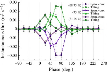
Figure 11. Comparison of the spanwise convective flux and vortex tilting terms calculated at the 68, 75 and 81 per cent span locations of the AR2 plunging case.
Overall, the behaviours of the shear-layer fluxes plotted in figure 10 are qualitatively similar for all three spanwise locations, as are the trends within the diffusive flux in the first half of the downstroke. However, during the second half of the downstroke, figures 10(a)–10(c) begin to show distinct variations in the diffusive fluxes. For comparison, the diffusive fluxes for the 68-ps, 75-ps, 81-ps and AR4 cases are plotted together in figure 12. Due to the small difference in control region locations between the AR4 and AR2 cases, the AR4 data have been recalculated using the boundaries of the AR2 control region to allow for a more relevant comparison, and therefore the AR4 data vary slightly from those shown in figure 5. While the AR2 data vary significantly from the two-dimensional case in the first half of the downstroke, the similarity is greater after
 $\unicode[STIX]{x1D719}=0^{\circ }$
. The major deviations of the AR2 data from the AR4 case are analysed next in the context of vorticity evolution.
$\unicode[STIX]{x1D719}=0^{\circ }$
. The major deviations of the AR2 data from the AR4 case are analysed next in the context of vorticity evolution.

Figure 12. Comparison of the diffusive flux of vorticity calculated at the 68.75, 75 and 81.25 per cent span locations of the AR2 plunging case. Also plotted is the diffusive flux calculated for the AR4 plunging case.

Figure 13. Vorticity isocontours obtained at the 68.75 per cent span of the AR2 case.
4.3 Re-stabilization of the LEV
Figure 13 shows the evolution of the spanwise vorticity field and surface pressure gradients at the 68-ps location. The presence of a distinct OSV and the detachment of the LEV from the downstream boundary layer in figure 13(a) indicates that the LEV has rolled up by
 $\unicode[STIX]{x1D719}=0^{\circ }$
. A comparison of figures 4(f–i) and 13(a–c) demonstrates that the subsequent growth of the LEV between
$\unicode[STIX]{x1D719}=0^{\circ }$
. A comparison of figures 4(f–i) and 13(a–c) demonstrates that the subsequent growth of the LEV between
 $\unicode[STIX]{x1D719}=0^{\circ }$
and
$\unicode[STIX]{x1D719}=0^{\circ }$
and
 $\unicode[STIX]{x1D719}=45^{\circ }$
is qualitatively similar to the AR4 case. However, while figure 4(j) shows that the eruption of secondary vorticity continues until the LEV is completely detached from the leading-edge shear layer in the AR4 case, figure 13(d,e) indicate that such an eruption does not continue to progress in the 68-ps plane. Instead, re-stabilization of the LEV begins around
$\unicode[STIX]{x1D719}=45^{\circ }$
is qualitatively similar to the AR4 case. However, while figure 4(j) shows that the eruption of secondary vorticity continues until the LEV is completely detached from the leading-edge shear layer in the AR4 case, figure 13(d,e) indicate that such an eruption does not continue to progress in the 68-ps plane. Instead, re-stabilization of the LEV begins around
 $\unicode[STIX]{x1D719}=67.5^{\circ }$
, as the LEV retracts back into the boundary layer while the OSV also weakens. Figure 12 reveals that once the LEV actually reattaches to the downstream boundary layer at
$\unicode[STIX]{x1D719}=67.5^{\circ }$
, as the LEV retracts back into the boundary layer while the OSV also weakens. Figure 12 reveals that once the LEV actually reattaches to the downstream boundary layer at
 $\unicode[STIX]{x1D719}=90^{\circ }$
, the diffusive flux of vorticity plotted for the 68-ps case exhibits a plateau, causing it to diverge from the baseline trend which continues to decrease. We anticipate that the delay in the reduction of the diffusive flux is due to the removal of the OSV, yielding the opposite effect associated with the formation of the OSV in the AR4 case.
$\unicode[STIX]{x1D719}=90^{\circ }$
, the diffusive flux of vorticity plotted for the 68-ps case exhibits a plateau, causing it to diverge from the baseline trend which continues to decrease. We anticipate that the delay in the reduction of the diffusive flux is due to the removal of the OSV, yielding the opposite effect associated with the formation of the OSV in the AR4 case.
The flow fields from the 75-ps case are shown in figure 14, which also shows the LEV to have rolled up by
 $\unicode[STIX]{x1D719}=0^{\circ }$
. Flow evolution at the 75-ps location is very similar to that observed at the 68-ps location except that the reattachment of the LEV to the downstream boundary layer occurs earlier at the 75-ps location. Figure 14(e) shows that this process eventually leads to the LEV merging with the downstream boundary layer and the OSV being completely eliminated. Consulting the 75-ps data from figure 12 shows that, again, the re-stabilization of the LEV produces a temporary plateau in the diffusive flux, which persists until the LEV merges with the boundary layer at approximately
$\unicode[STIX]{x1D719}=0^{\circ }$
. Flow evolution at the 75-ps location is very similar to that observed at the 68-ps location except that the reattachment of the LEV to the downstream boundary layer occurs earlier at the 75-ps location. Figure 14(e) shows that this process eventually leads to the LEV merging with the downstream boundary layer and the OSV being completely eliminated. Consulting the 75-ps data from figure 12 shows that, again, the re-stabilization of the LEV produces a temporary plateau in the diffusive flux, which persists until the LEV merges with the boundary layer at approximately
 $\unicode[STIX]{x1D719}\approx 90^{\circ }$
.
$\unicode[STIX]{x1D719}\approx 90^{\circ }$
.
At the 81-ps location, figure 15 shows that the LEV reattaches to the downstream boundary layer by
 $\unicode[STIX]{x1D719}=22.5^{\circ }$
. While figure 15(a–c) depicts the elimination of the OSV, the size and position of the LEV remains qualitatively similar; yet figure 12 indicates that simply maintaining this reattaching LEV structure near the leading edge of the airfoil – in contrast to the detachment and subsequent reattachment observed at the more inboard locations – produces a significant increase in the diffusive flux of vorticity. This augmentation lasts until
$\unicode[STIX]{x1D719}=22.5^{\circ }$
. While figure 15(a–c) depicts the elimination of the OSV, the size and position of the LEV remains qualitatively similar; yet figure 12 indicates that simply maintaining this reattaching LEV structure near the leading edge of the airfoil – in contrast to the detachment and subsequent reattachment observed at the more inboard locations – produces a significant increase in the diffusive flux of vorticity. This augmentation lasts until
 $\unicode[STIX]{x1D719}\approx 67.5^{\circ }$
, after which there is a rapid drop in the diffusive flux that once again accompanies the merging of the LEV into the boundary layer. Presumably, an even larger diffusive flux would be achieved at somewhat further outboard locations wherein the three-dimensionality of the flow is able to further mitigate the roll up of the LEV, rendering the flow more representative of an ideal inviscid flow with strong leading-edge suction. It should be noted that amplifying the diffusive flux of vorticity in this manner essentially correlates to the production of lower pressures on the leading edge of the wing, thereby enhancing lift or thrust due to the leading-edge suction.
$\unicode[STIX]{x1D719}\approx 67.5^{\circ }$
, after which there is a rapid drop in the diffusive flux that once again accompanies the merging of the LEV into the boundary layer. Presumably, an even larger diffusive flux would be achieved at somewhat further outboard locations wherein the three-dimensionality of the flow is able to further mitigate the roll up of the LEV, rendering the flow more representative of an ideal inviscid flow with strong leading-edge suction. It should be noted that amplifying the diffusive flux of vorticity in this manner essentially correlates to the production of lower pressures on the leading edge of the wing, thereby enhancing lift or thrust due to the leading-edge suction.

Figure 14. Vorticity isocontours obtained at the 75 per cent span of the AR2 case.

Figure 15. Vorticity isocontours obtained at the 81.25 per cent span of the AR2 case.
The correlations between the weakening or elimination of the OSV and the concurrent maintenance or significant increase in the diffusive flux further support the conclusion, in § 3.2, that the presence of an OSV (or, equivalently, ‘roll up of the LEV’) limits the growth of the diffusive flux. Based on these results, it appears that harnessing the underlying transport mechanism (through passive or active means) such as to prevent the roll up of the LEV – as opposed to reversing the roll up of the LEV after it has occurred – would be the most effective way of augmenting the diffusive flux and increasing aerodynamic performance by affecting the pressure distribution underlying these effects.
Taking into account the observation made in § 3.2 that the diffusive flux is responsible for the initial roll up of the LEV and subsequent emergence of the secondary vortex, it is perhaps somewhat counterintuitive that the re-stabilization of the LEV coincides with the augmentation of the diffusive flux. Since increasing the diffusive flux of vorticity would effectively increase the amount of cross-cancellation that is occurring within the reattachment region, the fact that the LEV is still able to re-stabilize indicates there must be an additional source of negative vorticity downstream of the LEV that allows the reattachment region to reform. In order to reconcile these observations and develop a more complete understanding of the underlying physics, it is necessary to consider the spatial distribution of the three-dimensional mechanisms of vorticity transport near the surface of the wing. This is discussed in the next section.
4.4 Three-dimensional fluxes of vorticity
When regarded from the perspective of the vorticity transport framework, the re-stabilization process is simply the consequence of a source of negative vorticity downstream of the LEV that is large enough to overcome the augmented diffusive flux of (positive) vorticity, and thereby bridge the gap between the LEV and the attached boundary layer. Figure 11 demonstrated significant individual contributions to the total circulation by the tilting and spanwise convective fluxes. The question is whether the integrands in either of these terms has sufficiently large magnitude in the vicinity of the re-stabilization.
In order to characterize the effect of this three-dimensionality on the flow field, figures 16–18 depict isocontours of the total three-dimensional flux of vorticity for the three spanwise planes during the phase interval over which the LEV was observed to reattach. As with the vorticity contours, regions outlined in dashed contours (shaded in red in the online version) indicate positive values (i.e. source of positive vorticity or sink of negative vorticity), and regions outlined in solid contours (shaded in blue in the online version) indicate negative values.
Although there is negligible net effect on the total circulation, the isocontours clearly show how the three-dimensionality within the flow creates a source of negative vorticity (blue) near the surface of the airfoil and a sink of negative vorticity (red) within the bulk flow. So as to provide an appropriate reference, an additional grey outline has been superimposed upon these contours at the vorticity threshold of
 $\unicode[STIX]{x1D714}c/U_{\infty }=-5$
in order to identify the position of the LEV. Based on the placement of these sources and sinks with respect to the LEV, it becomes apparent that the three-dimensional fluxes of vorticity induce the reattachment of the LEV by increasing the concentration of negative vorticity near the surface and decreasing the concentration within the separated region of the LEV.
$\unicode[STIX]{x1D714}c/U_{\infty }=-5$
in order to identify the position of the LEV. Based on the placement of these sources and sinks with respect to the LEV, it becomes apparent that the three-dimensional fluxes of vorticity induce the reattachment of the LEV by increasing the concentration of negative vorticity near the surface and decreasing the concentration within the separated region of the LEV.

Figure 16. Total three-dimensional flux of vorticity isocontours from the 68-ps case.

Figure 17. Total three-dimensional flux of vorticity isocontours from the 75-ps case.

Figure 18. Total three-dimensional flux of vorticity isocontours from the 81-ps case.
The specific source of the re-stabilization flux is further elucidated by figures 19 and 20, which decomposes the total three-dimensional flux of vorticity from the 81-ps case into the spanwise convection and tilting terms respectively. The isocontours presented within these figures demonstrate that both mechanisms act to increase the vorticity value – or deplete the negative vorticity – within the bulk flow and provide a source of negative vorticity near the surface of the airfoil. However, figure 19 indicates that the spanwise convective flux is primarily responsible for the flux of negative vorticity near the wing surface, while figure 20 indicates that the tilting term provides the strongest effect in the bulk flow.

Figure 19. Isocontours from the 81-ps case depicting the spanwise convection of vorticity.

Figure 20. Isocontours from the 81-ps case depicting the tilting of vorticity.
The source of the three-dimensional flux that governs the re-stabilization can be understood by observing the flow viewing in the streamwise direction. Figure 21 presents isocontours of
 $x$
-vorticity and in-plane velocity vectors in the
$x$
-vorticity and in-plane velocity vectors in the
 $yz$
-plane at
$yz$
-plane at
 $x/c=0.166$
. The three horizontal lines depict the three spanwise locations being considered. The region of negative vorticity near the bottom of the domain is associated with the tip vortex and the positive region is the projection of the LEV, which has been distorted into the streamwise direction. Both figures illustrate how the three-dimensional deformation of the LEV leads to the formation of spanwise flow directed towards the root of the airfoil.
$x/c=0.166$
. The three horizontal lines depict the three spanwise locations being considered. The region of negative vorticity near the bottom of the domain is associated with the tip vortex and the positive region is the projection of the LEV, which has been distorted into the streamwise direction. Both figures illustrate how the three-dimensional deformation of the LEV leads to the formation of spanwise flow directed towards the root of the airfoil.

Figure 21. Isocontours of streamwise vorticity and velocity vectors within the
 $yz$
-plane at the 16.6 per cent chordwise location.
$yz$
-plane at the 16.6 per cent chordwise location.
Figure 9(a–e) shows that the vorticity field near the tip of the wing primarily exists as an attached boundary layer. That the spanwise convective flux causes this boundary layer near the tip to convect inboard is well represented by the fact that the negative isocontours within figure 19 take on a distribution that is coincident with the attached boundary layer. Based on this characterization, it can be understood that the re-stabilization of the LEV is caused by the spanwise convection of an attached boundary layer into the plane. Therefore, while the surface diffusive flux downstream of the LEV acts to deteriorate the connection between the LEV and the downstream boundary layer – and thus initiate the process of LEV roll up – the spanwise flux retards and reverses this process by providing an additional source of primary (negative) vorticity within this region.
Despite the fact that spanwise flow does not appear to affect the net circulation of the LEV, it must be emphasized that spanwise flow is necessary for the stabilization of the LEV. While the total three-dimensional transport of vorticity does not alter the net circulation in the control region, it can modify the vorticity field so that the LEV remains attached to the downstream boundary layer, resulting in an augmentation of the diffusive flux of vorticity and enhanced suction near the leading edge. The enhanced diffusive flux, must then contribute to the regulation and even reversal of LEV formation. It should be noted here that the role of the spanwise flow in this case is distinct from that to which stability of an LEV has been attributed by other authors (e.g. Ellington et al. Reference Ellington, van den Berg, Willmott and Thomas1996) on a rotating wing. In those cases, centrifugal pumping in the LEV core is hypothesized to diminish LEV circulation and thus balance the shear-layer flux to achieve a steady state. In the present case, the spanwise convective flux contributes to the redistribution of vorticity and the delay or reversal of vortex evolution since it counteracts the effects of the diffusive flux which still play a critical role in the vorticity evolution, just as it has been shown to be important in governing the circulation budget on a rotating blade (Wojcik & Buchholz Reference Wojcik and Buchholz2014b ).
5 Conclusions
Examination of the phase-averaged surface pressure measurements and distributions of spanwise vorticity revealed that the surface pressure gradient established by the nascent LEV produced a surface diffusive flux of vorticity that consumed the boundary layer in the region of reattachment downstream of the forming vortex. The ultimate detachment of the vortex from the downstream boundary layer was considered the ‘roll up’ of the LEV, after which significant positive vorticity would begin to accumulate, forming the secondary vortex, or OSV. The presence of the OSV created a pressure plateau upstream of the primary suction peak which regulated the diffusive flux after roll up of the LEV. Therefore, it appears that the diffusive flux of vorticity can only be increased while it is manifested as a sink of negative vorticity.
This process was found to be robust when considering the development of the LEV on a finite plunging wing of aspect ratio 2, in which three-dimensional effects were significant. Vorticity flux analyses were performed at three different spanwise locations on the wing and the associated vorticity fields of these planes were considered in parallel with surface pressure measurements. Analysis of the 68.75, 75 and 81.25 per cent spanwise locations provided three examples wherein the LEV was seen to reattach to the downstream boundary layer after it had previously rolled up. Figure 12 further revealed that this re-stabilization of the LEV led to the augmentation of the diffusive flux of vorticity from the surface of the wing. By examining the spatial distribution of the three-dimensional vorticity transport mechanisms, it was determined that an additional source of negative vorticity – predominantly via a spanwise convective flux – within the reattachment region was the source of this re-stabilization process. This served to validate and extend the conclusions from the nominally two-dimensional case, as it demonstrated that the roll up of the LEV – and appearance of the OSV – was governed by the local vorticity balance within the reattachment region. It also suggests that a judicious introduction of three-dimensionality through wing design or flow control can be used to regulate the development of the LEV and alter aerodynamic loads.
Acknowledgements
This work was supported, in part, by the Air Force Office of Scientific Research under award no. FA9550-11-1-00190 and FA9550-16-1-0107 and by the National Science Foundation under EPSCoR grant EPS1101284. The particle image velocimetry measurements used in the analysis of the AR2 plate were obtained by Dr A. Eslam Panah (Eslam Panah Reference Eslam Panah2014).


