


1. Introduction
Swirling flows are found in a variety of geophysical and engineering applications, including hurricanes, tornadoes, jet engines, turbopumps and combustion chambers. For sufficiently large values of the swirl number  $S$, a measure of the ratio of circumferential to axial inlet velocity components, vortex breakdown, characterized by the formation of an internal stagnation point and a reversed axial flow (Leibovich Reference Leibovich1978), is known to occur. Despite numerous theoretical investigations, the mechanism for vortex breakdown is not yet fully agreed upon, as discussed in a variety of review papers (Hall Reference Hall1972; Leibovich Reference Leibovich1978, Reference Leibovich1984; Escudier Reference Escudier1988; Althaus, Brücker & Weimer Reference Althaus, Brücker and Weimer1995; Lucca-Negro & O'Doherty Reference Lucca-Negro and O'Doherty2001). One such theory, proposed independently by Squire (Reference Squire1960) and Benjamin (Reference Benjamin1962), suggests that vortex breakdown can be attributed to a jump in the criticality of the flow and its ability to support infinitesimal standing waves. An alternative theory by Brown & Lopez (Reference Brown and Lopez1990) states that vortex breakdown occurs as the result of the production of negative azimuthal vorticity that follows from an initial divergence of the vortex core.
A portion of the difficulty in obtaining a comprehensive understanding of the phenomenon arises from the variety of swirl-production methods and geometrical configurations studied. Controlled experiments have been performed in pipes and containers with a rotating end wall, while more recently, unconfined swirling flows have been studied and were found to exhibit entirely new forms of breakdown. The considerations in the present work will focus specifically on unconfined swirling jets, for which a round swirling jet core with a stagnant or slow swirl-free coflow discharges into an open atmosphere.
The first studies that were motivated by applications to combustion assumed constant density and focused on the turbulent regime. Chigier & Chervinsky (Reference Chigier and Chervinsky1967) calculated the spreading and entrainment of swirling jets, fitting empirical equations to the measured flow for varying degrees of inflow swirl. By considering two separate inflow swirl profiles, Farokhi, Taghavi & Rice (Reference Farokhi, Taghavi and Rice1989) found that the use of a single integrated swirl parameter was insufficient to determine the onset of vortex breakdown. Coherent structures and instabilities later became a focus of experimental investigations (Panda & McLaughlin Reference Panda and McLaughlin1994; Oberleithner et al. Reference Oberleithner, Sieber, Nayeri, Paschereit, Petz, Hege, Noack and Wygnanski2011, Reference Oberleithner, Paschereit, Seele and Wygnanski2012). Despite these studies, the fundamental physical aspects determining the onset of breakdown remain elusive, and progress can be made by analysing the laminar regime, which is the focus of this paper. Vortex breakdown in turbulent flows exhibits some phenomena not addressed here and requires a number of modelling hypotheses for its analysis.
The seminal experimental investigation by Billant, Chomaz & Huerre (Reference Billant, Chomaz and Huerre1998) unveiled the existence of two distinct types of vortex breakdown. Besides the well-documented bubble state, they found a new cone configuration in which the vortex takes the form of an open conical sheet. These two breakdown modes, axisymmetric for  $Re \leq 400$, experience transitions into corresponding asymmetrical states for sufficiently large Reynolds numbers, for which the stagnation point displays a precessing motion around the jet axis in a direction co-rotating with respect to the upstream vortex flow. Conical breakdown has also been observed in the same experimental apparatus by Gallaire, Rott & Chomaz (Reference Gallaire, Rott and Chomaz2004), and although not explicitly indicated, signs of conical breakdown were apparent in the experimental investigation by Liang & Maxworthy (Reference Liang and Maxworthy2005). Based on these observations, a critical swirl number
  $S^*$ can be defined as the lowest swirl number at which each breakdown first occurs as the swirl is gradually increased, and the subscripts
  $B$ and
  $C$ are used to denote the transition to the bubble and cone states. In the remainder of this paper, the term transition refers to a change in the state of the solution to the governing equations.
The axisymmetric numerical simulations conducted by Fitzgerald, Hourigan & Thompson (Reference Fitzgerald, Hourigan and Thompson2004) were able to reproduce the conical breakdown studied experimentally by Billant et al. (Reference Billant, Chomaz and Huerre1998). They also found that for sufficiently large values of the Reynolds number the flow became unstable directly, and bubble breakdown was bypassed. Moise & Mathew (Reference Moise and Mathew2019) studied numerically the range of existence and the structures of the bubble and cone through a series of three-dimensional time-dependent simulations at fixed Reynolds number and differing  $S$, beginning with a particular initial flow field defined by the inlet boundary condition profile in (2.8) prescribed at all axial locations. At the critical value
  $S^*_B$, the smooth pre-breakdown state was found to experience a transition to a bubble state upon breakdown. Further increase in
  $S$ revealed a second critical swirl number
  $S^*_C$, at which the bubble opened rapidly into a conical structure. For moderate swirl, the conical sheet exhibited a near-90
 $^{\circ}$ opening angle, enclosing a single recirculation zone. For larger values of the inflow swirl, a wide-open cone appeared with increasing values of
  $S$, as the sheet turned perpendicular to the jet axis at an off-axis location, bending upstream at large radial distances for larger
  $S$; it was not determined how abrupt the transition from the cone to the wide-open cone was because the computational expense of wide-open-cone simulations prevented computations from being performed in sufficiently small increments of
  $S$.
$S$.
Hysteresis, in which transitions occur at different values of  $S$, depending on whether
  $S$ is being increased or decreased, with the initial flow field taken to be the steady-state flow field at the previous value of
  $S$, was identified experimentally by Billant et al. (Reference Billant, Chomaz and Huerre1998) and also studied numerically by Moise (Reference Moise2020) through time-dependent inflow-swirl computations in the configuration of Moise & Mathew (Reference Moise and Mathew2019). These three-dimensional time-dependent computational results confirmed the bi-stability of the bubble and the cone, and emphasized that the value of
  $S^*$ at which transition occurs may depend, in general, on the initial conditions. Douglas, Emerson & Lieuwen (Reference Douglas, Emerson and Lieuwen2021) used bifurcation analysis to study the stability and dynamics of fully-developed swirling jets in a slightly different configuration; their steady, axisymmetric base-flow calculations identified all three forms of breakdown: bubble, cone and wide-open cone (referred to as a wall-jet in that study).
Unlike the previous constant-density studies, the density in a combustion chamber exhibits large spatial variations, exceeding a factor of five, associated with the temperature changes induced by the chemical heat release. Vortex breakdown is used to stabilize the flame by providing a low-velocity region preheated by the combustion products recirculating from downstream (Huang & Yang Reference Huang and Yang2009; Candel et al. Reference Candel, Durox, Schuller, Bourgouin and Moeck2014). There is interest, therefore, in characterizing effects of varying density on vortex breakdown of laminar jets, extending the previous constant-density analyses to gas-jet configurations with jet-to-ambient density ratios that differ from unity. Such effects were investigated experimentally by Adzlan & Gotoda (Reference Adzlan and Gotoda2012) for a coaxial configuration involving either an air jet or a carbon dioxide jet, both discharging into an air coflow. The experiments revealed that the heavier carbon dioxide jet exhibits a greater degree of flow divergence and lower critical swirl numbers than the air jet, and that augmenting the coflow velocity decreases the flow divergence and tends to suppress vortex breakdown.
The stability of low-Mach-number variable-density swirling jets has also been considered because of its influence on the precessing vortex core (PVC) in combustion. The convective/absolute stability of a typical bubble breakdown encountered in lean premixed combustion was studied by Manoharan et al. (Reference Manoharan, Hansford, O'Connor and Hemchandra2015). The authors showed that the baroclinic torque acted to stabilize the absolute first ( $m=1$) precessing mode, in agreement with the suppression of the PVC encountered in flames. Their later work (Manoharan et al. Reference Manoharan, Frederick, Clees, O'Connor and Hemchandra2020) further clarifies aspects of PVC in turbulent flows. Rukes et al. (Reference Rukes, Sieber, Paschereit and Oberleithner2016) identified experimentally a similar suppression of the global mode by implementing a heating source near the breakdown.
The present work employs theoretical and numerical techniques to study vortex breakdown in variable-density laminar swirling jets. Unlike the experimental analysis by Adzlan & Gotoda (Reference Adzlan and Gotoda2012), our work addresses a wide range of jet-to-ambient density differences and provides a systematic approach to identifying the onset of both forms of breakdown, which has not previously been done. To test the methods and investigate possible quantitative differences from the results published previously for constant-density swirling jets, the flow conditions considered include, in particular, those of the previous numerical investigations (Ruith, Chen & Meiburg Reference Ruith, Chen and Meiburg2004; Moise & Mathew Reference Moise and Mathew2019; Moise Reference Moise2020). For low-Mach-number gaseous jets considered here, differences in density emerge in connection with differences in composition or temperature between the jet and the ambient gas. We focus on the latter by considering the particular case of a jet discharging into an atmosphere of the same gas at a different ambient temperature, the transport-property variations of the gas taken to be those of air. Since the composition is uniform, the density becomes inversely proportional to the temperature, as follows from the equation of state, so that the boundary temperatures are related to the jet-to-ambient density ratio  $\varLambda$.
The approach in the analysis and the organization of the paper are as follows. The problem is formulated in § 2 with the governing equations and inflow boundary conditions. Critical vortex breakdown conditions for axisymmetric variable-density jets are derived in § 3 by application of different theoretical considerations. This section includes comparisons of predictions of  $S^*_B$ based on the so-called quasi-cylindrical approximation (Hall Reference Hall1967) with those obtained by numerical integration of the steady axisymmetric Navier–Stokes (NS) equations for large values of the Reynolds number. It is found that the steady NS computations are incapable of detecting conical breakdown, so the results of unsteady NS simulations are presented in § 4 to test the theoretical and steady predictions of
  $S^*_B$ as well as the theoretical predictions of
  $S^*_C$. Consistent with the intended focus on axisymmetric flow configurations, axisymmetric equations are employed in the unsteady simulations, which is beneficial in view of the high computational cost associated with running fully three-dimensional simulations across the entire range of
  $\varLambda$ and
  $S$ to be investigated. For large Reynolds numbers in the unsteady calculations, the flow becomes unstable and the pre-breakdown state transitions directly to the cone, bypassing the bubble state. To allow comparisons with the theoretical predictions that assume steady flow, the jet Reynolds number is modified with
  $\varLambda$ so that the flow remains stable. Finally, concluding remarks are given in § 5.
2. Formulation
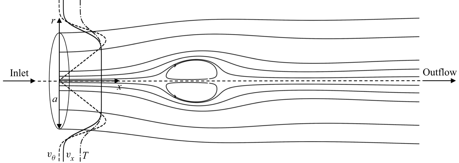
A schematic of the unconfined axisymmetric swirling jet and coordinate system considered is shown in figure 1.

Figure 1. The swirling jet investigated here. The plot shows the velocity and temperature profiles at the inlet, evaluated from (2.8) and (2.10) with  $\delta =0.2$ and
  $\epsilon =0.1$, and the streamlines (projected onto the meridional plane) corresponding to the flow with
  $S=1.5$,
  $\varLambda =1/2$ and
  $Re=111$, a configuration for which vortex breakdown leads to a bubble state.
2.1. Governing equations
The standard dimensional variables, denoted by  $'$, are made dimensionless in the following way. The jet radius
  $a$ and axial velocity
  $U_j$ are used to scale the time
  $t=t'/(a/U_j)$, cylindrical coordinates
  $(x,\theta,r)=(x'/a,\theta,r'/a)$, and velocity components
  $\boldsymbol {v}=(v_x,v_\theta,v_r)=(v'_x/U_j,v'_\theta /U_j,v'_r/U_j)$. The temperature, density, viscosity and thermal conductivity are scaled with their jet values to give the dimensionless variables
  $T=T'/T_j$,
  $\rho =\rho '/\rho _j$,
  $\mu =\mu '/\mu _j$ and
  $k=k'/k_j$. The axisymmetric NS equations are written for constant specific heat
  $c_p$ in the standard low-Mach-number non-dimensional form
 $$\begin{gather} \frac{\partial \rho}{\partial t}+ \boldsymbol{\nabla} \boldsymbol{\cdot} (\rho \boldsymbol{v})=0 , \end{gather}$$
 $$\begin{gather}\rho \left(\frac{\partial \boldsymbol{v}}{\partial t}+ \boldsymbol{v} \boldsymbol{\cdot} \boldsymbol{\nabla} \boldsymbol{v}\right)={-}\boldsymbol{\nabla} p + \frac{1}{{{Re}}} \boldsymbol{\nabla} \boldsymbol{\cdot} \tau , \end{gather}$$
 $$\begin{gather}\rho \left(\frac{\partial T}{\partial t}+ \boldsymbol{v} \boldsymbol{\cdot} \boldsymbol{\nabla} T\right)=\frac{1}{{{Re}} \, {{Pr}}} \boldsymbol{\nabla} \boldsymbol{\cdot} (k \boldsymbol{\nabla} T), \end{gather}$$
where  $Pr=\mu _j c_p/k_j=0.72$ is the Prandtl number evaluated in the jet stream,
  $\tau =\mu (\boldsymbol {\nabla } \boldsymbol {v} + \boldsymbol {\nabla } \boldsymbol {v}^T)$ is the dimensionless non-isotropic component of the viscous stress tensor, and
  $p$ represents the sum of the pressure difference with respect to the ambient value and the isotropic component of the viscous stress tensor (scaled with the characteristic dynamic pressure
  $\rho _j U_j^2$). The jet Reynolds number
 \begin{equation} {{Re}}=\frac{\rho_j U_j a}{\mu_j} \end{equation}
is defined based on the jet radius and velocity, and the properties of the jet. For the low Mach numbers considered here, the small pressure differences can be neglected when writing the equation of state
 \begin{equation} \rho T=1. \end{equation}
The viscosity and thermal conductivity are assumed to vary with temperature according to the power-law expressions
 \begin{equation} \mu=k=T^{\sigma}, \end{equation}
with a value  $\sigma =0.7$ selected for the exponent, as is appropriate for air.
2.2. Inlet boundary conditions
Similar to the previous numerical studies (Ruith et al. Reference Ruith, Chen and Meiburg2004; Moise & Mathew Reference Moise and Mathew2019; Moise Reference Moise2020), we focus on an inner swirling jet under solid-body rotation with angular speed  $\varOmega$ surrounded by a small swirl-free coaxial stream with velocity
  $\epsilon U_j$; the coflow parameter
  $\epsilon$ here was
  $\alpha ^{-1}$ in the previous studies. The swirl number is chosen as the ratio of the circumferential to axial velocity at the edge of a uniform-axial-velocity jet in solid-body rotation and can be defined by
 \begin{equation} S=\frac{\varOmega a}{U_j}. \end{equation}
To facilitate computations, smooth radial distributions of axial and azimuthal velocity components  $v_x$ and
  $v_\theta$, given by the so-called Maxworthy profiles (Ruith et al. Reference Ruith, Chen and Meiburg2004)
 \begin{equation} \frac{v_x-\epsilon}{1-\epsilon}=\frac{v_\theta}{S r}=\frac{1}{2} {\rm erfc}\left( \frac{r-1}{\delta}\right), \quad v_r=0, \end{equation}
were prescribed at the inflow boundary  $x=0$, and the radial velocity
  $v_r$ was set equal to zero. Here
  $r$ is the radial distance to the axis,
  ${\rm erfc}$ is the complementary error function, and
  $\delta$ represents the relative thickness of the mixing layer separating the jet from the ambient coflow. Note that the canonical case of a jet with uniform velocity and solid-body rotation discharging into a stagnant atmosphere is recovered from the above expressions by taking the limit
  $\epsilon \ll 1$ and
  $\delta \ll 1$.
As discussed by Moise & Mathew (Reference Moise and Mathew2019), the use of a prescribed velocity field at the inlet plane is questionable for cases when the breakdown occurs near the inlet, since the downstream evolution then may be expected to modify the flow field upstream from this boundary, but accounting for such effects would complicate computations considerably. All of the computations in Moise & Mathew (Reference Moise and Mathew2019) and Moise (Reference Moise2020) were for  $\delta =0.2$ and
  $\epsilon =0.01$, but other values are to be addressed as well in the present work.
For the case considered, a jet at temperature  $T_j$ is surrounded by an ambient coflow at temperature
  $T_a$, so that the boundary temperatures are related to the jet-to-ambient density ratio
  $\rho _j/\rho _a$ by
 \begin{equation} \varLambda=\frac{\rho_j}{\rho_a}=\frac{T_a}{T_j}. \end{equation}
For consistency, the same mixing-layer thickness  $\delta$ is introduced in defining the associated inflow boundary temperature profile
 \begin{equation} \frac{T-\varLambda}{1-\varLambda}=\frac{1}{2} {\rm erfc}\left( \frac{r-1}{\delta}\right). \end{equation}
The inlet boundary conditions (2.8) and (2.10) are shown in figure 1, along with a representative computational result of a bubble breakdown.
3. Theoretical predictions of vortex breakdown
Before presenting results of numerical computations, it is of interest to determine the critical swirl numbers  $S^*_B$ and
  $S^*_C$ by applying different vortex breakdown theories. Besides classical theories, a new criterion will be derived on the basis of considerations of flow alignment. Most predictions pertain to jets with uniform velocity and solid-body rotation discharging into a stagnant atmosphere, corresponding to values of
  $\epsilon =0$ and
  $\delta =0$ in (2.8) and (2.10). We begin below by reviewing results based on inviscid flow, and address influences of molecular transport later.
3.1. Outermost bounds of critical swirl numbers
We begin by addressing predictions based on purely inviscid flow for a steady cylindrical jet having uniform axial velocity  $v_x=1$ and solid-body rotation
  $v_\theta =S r$ surrounded by stagnant fluid with uniform pressure
  $p=0$. The transverse pressure distribution across the jet at the inlet plane,
 \begin{equation} p(r)={-} \frac{S^2}{2} (1-r^2), \end{equation}
follows from integrating the simplified momentum equation  $\partial p/\partial r=v_\theta ^2/r$ subject to the condition
  $p=0$ at
  $r=1$.
As shown by Billant et al. (Reference Billant, Chomaz and Huerre1998), a criterion for vortex breakdown can be derived by investigating the conditions needed for emergence of a stagnation point. Conservation of head along the axis yields  $p_0=(1-S^2)/2$ for the pressure at the stagnation point. In the conical type of breakdown, the velocities inside the recirculating conical region lying downstream from the stagnation point are small. If they are neglected, then the pressure inside the cone must be uniform, equal to
  $p_0$, and if the conical region extends to infinity, then
  $p_0=0$, thereby yielding the breakdown prediction
  $S^*_C=1$ for conical breakdown. For bubble breakdown, it is reasoned (Billant et al. Reference Billant, Chomaz and Huerre1998) that the stagnation pressure cannot exceed the surrounding pressure, leading to the weaker condition
  $p_0 \le 0$ and associated lower bound
 \begin{equation} S^*_B \ge 1, \end{equation}
for the critical swirl number.
Alternative breakdown predictions can be derived by analysing the criticality of the jet flow, that is, its ability to support infinitesimal stationary disturbances in the form of sinusoidal waves (Squire Reference Squire1960; Benjamin Reference Benjamin1962). As explained by Hall (Reference Hall1972), the analysis considers stationary axisymmetric disturbances described by the perturbation stream function  $F(r) e^{\gamma x}$, where the function
  $F$ must satisfy the Sturm–Liouville problem
 \begin{equation} \frac{{\rm d}^2 F}{{\rm d} r^2}-\frac{1}{r}\,\frac{{\rm d} F}{{\rm d} r}+\left(\gamma^2 - \frac{1}{v_x}\,\frac{{\rm d}^2 v_x}{{\rm d} r^2}+ \frac{1}{r v_x}\,\frac{{\rm d} v_x}{{\rm d} r} + \frac{1}{r^3 v_x^2}\, \frac{{\rm d} (r v_\theta)^2}{{\rm d} r} \right)F=0, \quad F(0)=F(1)=0.\end{equation}
For the case  $v_x=1$ and
  $v_\theta =S r$ considered here, the problem can be solved to give the eigensolutions
  $F_n=r J_1[(\gamma _n^2+ 4 S^2)^{1/2} r]$ and corresponding eigenvalues
  $\gamma _n^2=\xi _n^2-4S^2$, where
  $\xi _n$ are the zeros of the Bessel function of order unity,
  $J_1$. If all eigenvalues
  $\gamma _n^2$ are positive, then the flow is supercritical, whereas existence of at least one negative eigenvalue implies that the flow is subcritical, in that it can support stationary disturbances. Since the smallest eigenvalue
  $\gamma ^2_1=\xi _1^2-4S^2$ is determined by the first zero
  $\xi _1 \simeq 3.8317$, the transition from supercritical to subcritical is associated with the boundary value
  $S=\xi _1/2\simeq 1.916$ at which
  $\gamma ^2_1=0$.
Different interpretations of the significance of the critical state for jet vortex breakdown have been proposed, as discussed by Hall (Reference Hall1972). According to Squire (Reference Squire1960), vortex breakdown must occur when the flow is exactly critical, so that in that case,  $S^* \simeq 1.916$ provides a precise prediction for the breakdown swirl number. In contrast, Benjamin (Reference Benjamin1962) characterizes breakdown as a sudden transition from supercritical to subcritical flow. No precise prediction for
  $S^*$ follows from this alternative interpretation, the value
  $S^* \simeq 1.916$ being instead an upper bound. Based on these ideas, therefore, it can be inferred that the swirl number for the discharging jet must satisfy the constraint
 \begin{equation} S^* \le 1.916, \end{equation}
as needed for the flow upstream from the breakdown location to be either critical ( $S=1.916$) or supercritical (
 $S<1.916$).
3.2. Transition to the bubble: theoretical
Hall (Reference Hall1967) proposed an entirely different approach to the computation of vortex breakdown based on the failure of the quasi-cylindrical (QC) approximation of viscous axisymmetric flow. This approach applies specifically to bubble breakdown, when the flow upstream from the stagnation point is steady and varies only gradually in the axial direction. Hall's approach (Hall Reference Hall1967) builds on ideas developed in connection with two-dimensional boundary layers, where the separation is predicted based on the failure of the downstream-marching numerical integration of the boundary layer equations. For swirling flows, it is reasoned that if in the course of the calculation of a QC vortex core for a given value of  $S$ the results develop a singularity at a given location, characterized by rapid increase of axial gradients and radial velocities, then there must also be appreciable axial gradients at that location in the associated real vortex core, corresponding to vortex breakdown. In this approximation, the predicted critical swirl number
  $S^*_B$ (the smallest value of
  $S$ for which a singularity develops), is independent of
  $Re$. Results will be computed below for different values of the jet-to-ambient density ratio
  $\varLambda$, thereby complementing previous results pertaining to constant-density jets (Revuelta, Sánchez & Liñán Reference Revuelta, Sánchez and Liñán2004) and light compressible jets (Gallardo-Ruiz, Pino & Fernandez Reference Gallardo-Ruiz, del Pino and Fernandez-Feria2010).
3.2.1. Slender jet equations
For the moderately large values of  ${{Re}}$ considered, the jet remains slender for values of
  $S$ smaller than
  $S^*_B$, which is of order unity. The slender flow includes a development region
  $x' \sim {{Re}} a$ where the axial velocity
  $v'_x$ is of order
  $U_j$ and the radial velocity
  $v'_r$ is of order
  $U_j/{{Re}} \ll U_j$. If the Reynolds number is also sufficiently low for the flow to remain stable, then the velocity in the far field approaches the well-known Schlichting solution (von Schlichting Reference von Schlichting1933), with accompanying weak swirling motion given by the Görtler–Loitsianskii solution (Loitsianskii Reference Loitsianskii1953; Görtler Reference Görtler1954).
To facilitate the presentation, it is useful to describe the azimuthal motion in terms of the dimensionless circulation per unit azimuthal angle  $\varGamma = (r' v'_\theta )/(\varOmega a^2)=r v_\theta /S$ and use the characteristic scales of the slender jet development region to define a rescaled axial distance
  $\hat {x}=x'/({{Re}}\,a)=x/{{Re}}$ and a rescaled radial velocity
  $\hat {v}_r=v'_r/[(\mu _j/\rho _j)/a]={{Re}} v_r$. In terms of these new variables, the conservation equations (2.1)–(2.3) can be written in the steady form
 \begin{align} \frac{\partial}{\partial \hat{x}} (\rho v_x)+\frac{1}{r}\,\frac{\partial}{\partial r}(\rho r \hat{v}_r) &=0, \end{align}
 \begin{align} \rho \left( v_x \frac{\partial v_x}{\partial \hat{x}} +\hat{v}_r \frac{\partial v_x}{\partial r}\right) &={-}\frac{\partial p}{\partial \hat{x}} + \frac{1}{r}\,\frac{\partial}{\partial r}\left(\mu r \frac{\partial v_x}{\partial r} \right) \nonumber\\ & \quad +\frac{1}{{{Re}}^2} \left[\frac{\partial}{\partial \hat{x}}\left(2 \mu \frac{\partial v_x}{\partial \hat{x}}\right) +\frac{1}{r}\,\frac{\partial}{\partial r}\left(\mu r \frac{\partial \hat{v}_r}{\partial r} \right) \right], \end{align}
 \begin{align} \rho \left(v_x \frac{\partial \hat{v}_r}{\partial \hat{x}} +\hat{v}_r \frac{\partial \hat{v}_r}{\partial r} \right)&= {{Re}}^2\left(S^2 \rho \frac{\varGamma^2}{r^3}- \frac{\partial p}{\partial r} \right)+\frac{1}{r}\,\frac{\partial}{\partial r}\left(2 \mu r \frac{\partial \hat{v}_r}{\partial r}\right) \nonumber\\ &\quad -2\mu \frac{\hat{v}_r}{r^2} +\frac{\partial}{\partial \hat{x}} \left(\mu \frac{\partial v_x}{\partial r} \right) +\frac{1}{{{Re}}^2}\,\frac{\partial}{\partial \hat{x}}\left(\mu \frac{\partial \hat{v}_r}{\partial \hat{x}} \right), \end{align}
 \begin{align} \rho \left(v_x \frac{\partial \varGamma}{\partial \hat{x}} +\hat{v}_r \frac{\partial \varGamma}{\partial r} \right)&= \frac{1}{r}\,\frac{\partial}{\partial r}\left(\mu r \frac{\partial \varGamma}{\partial r}-2\mu \varGamma \right) +\frac{1}{{{Re}}^2}\,\frac{\partial}{\partial \hat{x}}\left(\mu \frac{\partial \varGamma}{\partial \hat{x}} \right), \end{align}
 \begin{align} \rho \left(v_x \frac{\partial T}{\partial \hat{x}} +\hat{v}_r \frac{\partial T}{\partial r} \right)&= \frac{1}{r}\,\frac{\partial}{\partial r}\left(\frac{k}{{{Pr}}}\,r\,\frac{\partial T}{\partial r}\right) +\frac{1}{{{Re}}^2}\,\frac{\partial}{\partial \hat{x}}\left(\frac{k}{{{Pr}}}\, \frac{\partial T}{\partial \hat{x}} \right), \end{align}
which will be useful in analysing molecular-transport effects.
3.2.2. Quasi-cylindrical equations and boundary conditions
In the absence of breakdown, the flow is slender, so that with the scalings selected in (3.5)–(3.9), all dimensionless variables and their derivatives remain of order unity. Steady solutions can be described by integrating for  $\hat {x}>0$ the QC equations
 $$\begin{gather} \frac{\partial}{\partial \hat{x}} (\rho v_x)+\frac{1}{r}\,\frac{\partial}{\partial r}(\rho r \hat{v}_r)= 0, \end{gather}$$
 $$\begin{gather}\rho \left(v_x \frac{\partial v_x}{\partial \hat{x}} +\hat{v}_r \frac{\partial v_x}{\partial r} \right)={-}\frac{\partial p}{\partial \hat{x}} + \frac{1}{r}\,\frac{\partial}{\partial r}\left(\mu r \frac{\partial v_x}{\partial r} \right), \end{gather}$$
 $$\begin{gather}0= S^2 \rho \frac{\varGamma^2}{r^3}- \frac{\partial p}{\partial r}, \end{gather}$$
 $$\begin{gather}\rho \left(v_x \frac{\partial \varGamma}{\partial \hat{x}} +\hat{v}_r \frac{\partial \varGamma}{\partial r} \right)= \frac{1}{r}\,\frac{\partial}{\partial r}\left(\mu r \frac{\partial \varGamma}{\partial r}-2\mu \varGamma \right), \end{gather}$$
 $$\begin{gather}\rho \left(v_x \frac{\partial T}{\partial \hat{x}} +\hat{v}_r \frac{\partial T}{\partial r} \right)= \frac{1}{r}\,\frac{\partial}{\partial r}\left(\frac{k}{{{Pr}}}\,r\,\frac{\partial T}{\partial r}\right), \end{gather}$$
obtained by taking the limit  ${{Re}} \gg 1$ in (3.5)–(3.9), with boundary conditions
 \begin{equation} \frac{v_x-\epsilon}{1-\epsilon}=\frac{\varGamma}{r^2}= \frac{T-\varLambda}{1-\varLambda}=\frac{1}{2} {\rm erfc} \left( \frac{r-1}{\delta}\right) \quad {\rm at} \ \hat{x}=0,\end{equation}
and
 \begin{equation} v_x-\epsilon=\varGamma=T-\varLambda=0 \quad {\rm as} \ r \to \infty, \end{equation}
both consistent with (2.8) and (2.10), supplemented with
 \begin{equation} \frac{\partial v_x}{\partial r}=\hat{v}_r=\varGamma=\frac{\partial T}{\partial r}=0 \quad {\rm at} \ r=0, \end{equation}
corresponding to the regularity condition at the axis.
3.2.3. Preliminary considerations
Radial integration of a combination of (3.11) and (3.14) provides the integral momentum balance
 \begin{equation} \int_0^\infty 2 r [\rho v_x(v_x-\epsilon) +p] \,{\rm d}r=M, \end{equation}
to be satisfied by the QC solution at any downstream location. The constant  $M$ is the so-called flow force, which can be evaluated at
  $\hat {x}=0$ using the velocity and temperature profiles (3.15) along with the corresponding boundary pressure distribution
  $p=-S^2 \int _r^\infty \rho \varGamma ^2/r^3 \, {\rm d}r$, obtained from (3.12). Since the pressure is negative, the value of
  $M$ decreases for increasing values of
  $S$. The condition
  $M>0$ imposes a natural upper limit on the value of
  $S$ for which the flow can develop downstream as a slender jet. For example, for the canonical case
  $\epsilon =\delta =0$, the flow force reduces to
 \begin{equation} M=1-S^2/4, \end{equation}
so values of  $S>2$ necessarily result in vortex breakdown, an upper bound in quantitative agreement with Benjamin's criterion (3.4).
3.2.4. Quasi-cylindrical predictions
The problem defined in (3.10)–(3.17) was integrated numerically for given values of  $S$ and
  $\varLambda$ by marching downstream from
  $\hat {x}=0$. The integration of the parabolic QC equations employed an implicit method using first-order/second-order approximation schemes for axial/radial derivatives, respectively. At each axial location, a Newton method is first utilized to compute
  $v_x$ and
  $\hat {v}_r$ from (3.10) and (3.11). Next, (3.13) and (3.14) are integrated to determine
  $\varGamma$ and
  $T$, and the result is used to compute the radial distribution of pressure from (3.12). A fixed-point iteration scheme is applied until convergence is achieved. Typical values of the grid spacing are
  $\delta r = 10^{-2}$ and
  $\delta \hat {x} = 10^{-4}$, with finer grids being needed for increasing
  $S$.
$S$.
The typical evolution of the axial velocity along the axis is shown in the solid curves of figure 2 for the constant-density jet ( $\varLambda =1$) with
  $\epsilon =0.01$ and
  $\delta =0.2$ (the dashed curves correspond to results of integrations of the steady NS equations, to be discussed below). The adverse pressure gradient induced by the jet swirl leads to a significant deceleration of the flow that becomes more pronounced for larger values of
  $S$. The non-monotonic velocity variation observed at
  $S=1.31$, associated with the emergence of a small region of swelling centred around
  $\hat {x} \simeq 0.03$, has been reasoned to characterize pre-breakdown conditions in the numerical simulations of Moise & Mathew (Reference Moise and Mathew2019). The numerical integration could no longer converge for
  $S=1.312$, with the axial gradients developing a singularity at
  $\hat {x} \simeq 0.026$. According to Hall (Reference Hall1967), this breakdown of the QC approximation at a given downstream location identifies the critical swirl number
  $S^*_B$ as the pre-breakdown slender jet transitions to the bubble, an aspect of the problem to be explored further in § 3.2.5.


The critical swirl number  $S^*_B$ associated with the development of a singularity in the numerical integration was calculated for values of the density ratio in the range
  $0.1 \le \varLambda \le 10$, with results represented by curves in figure 3. Besides the canonical case
  $\epsilon =\delta =0$, integrations were performed for small coflow
  $\epsilon =0.01$ with two different values of the shear-layer thickness,
  $\delta =0.1$ and
  $\delta =0.2$. As can be seen, although the critical swirl number varies with
  $\varLambda$, the variation is not very pronounced, especially for
  $\delta = 0.2$ (the most gradual transition from the inner swirling jet to the outer non-swirling flow at the inlet), when small relative changes of order
  $4\,\%$ are observed as
  $\varLambda$ increases from
  $\varLambda =0.1$ to
  $\varLambda =10$. The decrease of
  $S^*_B$ with increasing
  $\varLambda$ for sharp entry conditions may be attributed to an increase of the centrifugal force with an increasing ratio of swirling-jet-fluid-to-ambient density.

Figure 3. The variation with  $\varLambda$ of the critical swirl number
  $S^*_B$ determined by the development of a singularity in the numerical integration of the QC problem (3.10)–(3.17) for
  $(\delta,\epsilon )=(0,0)$ (bottom curve),
  $(\delta,\epsilon )=(0.1,0.01)$ (intermediate curve) and
  $(\delta,\epsilon )=(0.2,0.01)$ (top curve). The crosses represent values of
  $S^*_B$ determined for
  $\varLambda =(1/5,1,5)$ from numerical integrations of the steady form of (2.1)–(2.3) with
  $(\delta,\epsilon )=(0.2,0.01)$ and different values of
  ${{Re}}$.
3.2.5. Comparisons with steady NS computations
The QC approximation assumes that the flow is steady and slender upstream from the breakdown point, which requires that the Reynolds number be moderately large, so that the laminar jet remains stable. Under such conditions, the bubble mode prevails when vortex breakdown first occurs on increasing the swirl number, so that the value  $S^*$ of
  $S$ at which the numerical integration of the QC equations fails, shown in figure 3, can be reasoned to correspond to the critical swirl number
  $S^*_B$.
To explore this aspect of the problem further and ascertain the predictive capabilities of the QC description, the results of the QC approximation were compared with numerical integrations of the steady NS equations (2.1)–(2.3) for a range of large values of  ${{Re}}$, shown in figure 4. The numerical integration employs a root-finding scheme involving a Newton–Raphson algorithm, thereby enabling the description of steady solutions even for large values of the Reynolds number for which the flow is unstable. This type of description is needed, for example, in base-flow computations for global linear stability analyses (see, for example, Moreno-Boza et al. (Reference Moreno-Boza, Coenen, Sevilla, Carpio, Sánchez and Liñán2016, Reference Moreno-Boza, Coenen, Carpio, Sánchez and Williams2018) for recent sample computations involving low-Mach-number variable-density flows). As in Moise & Mathew (Reference Moise and Mathew2019), this set of simulations employed the parametric values
  $\delta =0.2$ and
  $\epsilon =0.01$ for the inlet boundary profiles. The cylindrical computational domain used in the integrations and the boundary conditions applied on the lateral and outlet boundaries are those described in § 4.1 in connection with the accompanying unsteady computations.

Figure 4. The variation with streamwise distance  $\hat {x}=x/{{Re}}$ of the axial velocity determined numerically for
  $(\delta,\epsilon )=(0.2,0.01)$ and
  $\varLambda =(1/5,1,5)$ from integration of the QC problem (3.10)–(3.17) (solid curves) and from integration of the steady form of the axisymmetric NS equations (2.1)–(2.3) for selected values of
  ${{Re}}$. (a)
  $S=1.3$,
  $\varLambda = 1/5$, (b)
  $S=1.3$,
  $\varLambda = 1$, and (c)
  $S=1.3$,
  $\varLambda = 5$.
The asymptotic theory underlying the QC approximation envisions the QC velocity field as the limiting solution for  ${{Re}} \gg 1$ of the steady NS equations, provided that the flow remains slender. This fundamental assumption is tested in figure 4 by comparing the QC predictions of velocity distributions along the axis with solutions to the steady NS equations with
  $\varLambda =(1/5,1,5)$ and increasing values of
  ${{Re}}$. The value
  $S=1.3$ is selected for the swirl number, thereby placing the system near the breakdown conditions predicted by the QC approximation, represented by the top curve in figure 3. The comparisons exhibit the expected convergence when
  ${{Re}}$ increases. Close quantitative agreement of NS and QC results requires values of
  ${{Re}}$ that are higher for the cold jet
  $\varLambda =5$ than for the hot jet
  $\varLambda =1/5$, as is to be expected given the temperature dependence of the kinematic viscosity and the accompanying associated reduction in effective Reynolds number with increasing
  $\varLambda$ (see also the discussion in § 4.3).
To investigate the failure of the QC approximation, additional NS results corresponding to the constant-density jet with  ${{Re}}=800$ are presented in figure 2. For this large Reynolds number, the QC and NS profiles are virtually indistinguishable for
  $S=(0,0.8,1.2)$. The agreement deteriorates as the axial gradient increases for larger
  $S$. The QC velocity profile undergoes a rapid evolution as the swirl number increases from
  $S=1.3$, the case shown in the central panel of figure 4, with the profile for
  $S=1.31$ in figure 2 showing a local region of non-monotonic variation that serves as a precursor for the singularity developing when
  $S=1.312$. By way of contrast, the development of non-monotonicity in the NS velocity distribution occurs for slightly larger values of
  $S \simeq 1.33$ and results in the development of multiple streamwise oscillations, eventually leading to the emergence of a stagnation point along the axis, as the bubble first develops, with corresponding streamlines represented in figure 5. The observed streamline pattern, involving a standing wave downstream of the stagnation point, is indicative of transition from supercritical to subcritical flow, an aspect of the problem investigated in earlier studies (Oberleithner et al. Reference Oberleithner, Paschereit, Seele and Wygnanski2012; Moise & Mathew Reference Moise and Mathew2019).


The value  $S^*_B$ of
  $S$ at which the integrations of the steady NS solutions first exhibit a stagnation point along the axis was computed for
  $\delta =0.2$,
  $\epsilon =0.01$,
  $\varLambda =(1/5,1,5)$ and selected values of the Reynolds number. Results are compared in figure 3 with the QC predictions for
  $\delta =0.2$ and
  $\epsilon =0.01$ (i.e. the top curve of this figure). The results indicate that the
  $S^*_B$ predicted by the NS computations decreases for increasing
  ${{Re}}$, approaching from above the QC prediction, as may be expected from the stabilizing influence of viscosity.
To describe the growth of the steady bubble, the numerical integration was extended to values of  $S>S^*_B$. Contrary to Douglas et al. (Reference Douglas, Emerson and Lieuwen2021), who identified a steady cone, considering an inlet region having a Poiseuille axial velocity inflow and a wall preventing the external coflow, in our steady NS computations the bubble was seen to persist as the value of
  $S$ was increased beyond the critical transition value
  $S^*_C$ predicted by the unsteady simulations (to be discussed in § 4.5). The persistence of the bubble, consistent with the results of previous numerical studies addressing hysteresis (Moise Reference Moise2020; Moise & Mathew Reference Moise and Mathew2021), is illustrated in figure 6, which shows projected streamlines corresponding to
  $\varLambda =2$ and
  ${{Re}}=361$, for which
  $S^*_C=1.51$. Instead of transitioning to a cone, the bubble recirculation region in the steady computations increases in size until the Newton–Raphson algorithm fails to converge. For example, for
  $\varLambda =1$ and
  ${{Re}}=(100,200,400)$, convergence fails at
  $S=(1.895,1.958,1.968)$, values far larger than
  $S^*_C$ found in the theoretical predictions (§ 3.3) and the unsteady numerical simulations (§ 4.5). For
  $\varLambda =1/5$ and
  ${{Re}}=51$, similar convergence issues were encountered, and no steady solution was found for
  $S>1.75$. These observations indicate that for the specific boundary conditions considered in our analysis, the description of conical breakdown necessitates consideration of unsteady computations, to be addressed in § 4.

Figure 6. Projected streamlines superimposed on colour contours of temperature for  $\varLambda =2$ and
  ${{Re}}=361$ obtained from the steady NS simulations (b,d) and corresponding results obtained by time-averaging the solution of the unsteady NS computations (a,c). As
  $S$ is increased beyond the value
  $S^*_C=1.51$ predicted by the unsteady NS simulations (§ 4.5), the steady NS solutions (b,d) are unable to detect conical breakdown. (a)
  $S=1.47$, (b)
  $S=1.47$, (c)
  $S=1.55$, and (d)
  $S=1.55$.
3.3. Transition to the cone: theoretical
As shown in experiments (Billant et al. Reference Billant, Chomaz and Huerre1998) and numerical computations (Moise & Mathew Reference Moise and Mathew2019), flows undergoing conical breakdown exhibit near the inlet plane radial velocities  $v'_r$ that are comparable to
  $U_j$, with the stream surface bounding the jet opening up very rapidly. Correspondingly, the scaling
  $v'_r \sim U_j/{{Re}} \ll U_j$ used in (3.5)–(3.9), appropriate for slender jets, can be expected to fail when conical breakdown occurs, leading to diverging values of
  $\hat {v}_r=v'_r/(U_j/{{Re}})$ at the jet inlet. These considerations suggest that a theoretical prediction for the critical value
  $S^*_C$ associated with conical breakdown can be derived by investigating the structure of the flow near the inlet plane. To simplify the analysis and reduce the number of parameters in the results, attention is focused on the case
  $\delta = \epsilon = 0$. The near-field solution at distances
  $\hat {x} \ll 1$ will be shown to include an inviscid core extending over radial distances in the range
  $1 \ge 1-r \gg \hat {x}^{1/2}$ surrounded by a mixing layer of small thickness
  $\hat {x}^{1/2}$ centred at
  $r=1$. Matched asymptotic expansions will be used to describe the flow and determine the conditions at which conical divergence is first encountered.
3.3.1. The inviscid core
In the inviscid core, where  $T=1$ (and therefore
  $\rho =1)$, the perturbations to the initial inlet distributions are of the form
 \begin{gather} \left. \begin{gathered}
v_x-1=\hat{x}\,u_1(r)+\hat{x}^{3/2}\,u_2(r)+\cdots,\\
\hat{v}_r=v_1(r)+\hat{x}^{1/2}\,v_2(r)+\cdots, \\
p+S^2(1-r^2)/2=\hat{x}\,p_1(r)+\hat{x}^{3/2}\,p_2(r)+\cdots,
\\
\varGamma-r^2=\hat{x}\,g_1(r)+\hat{x}^{3/2}\,g_2(r)+\cdots.
\end{gathered} \right\} \end{gather}
\begin{gather} \left. \begin{gathered}
v_x-1=\hat{x}\,u_1(r)+\hat{x}^{3/2}\,u_2(r)+\cdots,\\
\hat{v}_r=v_1(r)+\hat{x}^{1/2}\,v_2(r)+\cdots, \\
p+S^2(1-r^2)/2=\hat{x}\,p_1(r)+\hat{x}^{3/2}\,p_2(r)+\cdots,
\\
\varGamma-r^2=\hat{x}\,g_1(r)+\hat{x}^{3/2}\,g_2(r)+\cdots.
\end{gathered} \right\} \end{gather}
The first-order corrections satisfy the linear equations
 \begin{equation} u_1+\frac{1}{r}\,\frac{{\rm d}}{{\rm d} r}(r v_1)=u_1+p_1=\frac{2 S^2}{r} g_1-\frac{{\rm d} p_1}{{\rm d} r}=g_1+2 r v_1=0, \end{equation}
which can be combined to give the second-order linear equation
 \begin{equation} r^2 \frac{{\rm d}^2 v_1}{{\rm d} r^2}+r \frac{{\rm d} v_1}{{\rm d} r}+(4 S^2 r^2-1) v_1=0. \end{equation}
Integration of (3.22) with boundary condition  $v_1(0)=0$ provides the normalized distribution
  $v_1(r)/v_1(1)=J_1(2 S r)/J_1(2 S)$ in terms of the unknown value of the transverse velocity at the jet surface
  $v_1(1)$, thereby yielding
 \begin{equation} u_1={-}p_1={-}2 S\,\frac{J_0(2 S r)}{J_1(2 S)}\,v_1(1) \quad {\rm and} \quad v_1={-}\frac{g_1}{2r}=\frac{J_1(2 S r)}{J_1(2 S)}\,v_1(1), \end{equation}
where  $J_0$ and
  $J_1$ represent Bessel functions of the first kind.
3.3.2. Chapman–Lessen mixing layer
The mixing layer that develops from the orifice rim, of characteristic thickness  $r-1 \sim \hat {x}^{1/2}$, admits a self-similar solution. The description is facilitated by introduction of the stream function
  $\psi$ for the axial and radial motion. The analysis employs a rescaled similarity coordinate
  $\eta =(r^2-1)/(2 \hat {x}^{1/2})$ along with expansions
  $\psi =\hat {x}^{1/2}\,F_0(\eta )+\hat {x}\,F_1(\eta )+\cdots$,
  $P=\hat {x}^{1/2}\,P_0(\eta )+\hat {x}\,P_1(\eta )+\cdots$,
  $\varGamma =G_0(\eta )+$
  $\hat {x}^{1/2}\,G_1(\eta )+\cdots$ and
  $T=T_0(\eta )+\hat {x}^{1/2}\,T_1(\eta )+\cdots$, with corresponding velocity components given by
  $\rho v_x= F'_0+\hat {x}^{1/2} F_1'+\cdots$ and
  $\rho \hat {v}_r r=\hat {x}^{-1/2} [\tfrac {1}{2}(\eta F_0'-F_0)+\hat {x}^{1/2} (\tfrac {1}{2}\eta F_1'-F_1)+\cdots ]$, where the prime is used to denote differentiation with respect to
  $\eta$. Introducing these expansions into (3.11)–(3.14) and collecting terms in decreasing powers of
  $\hat {x}$ provides a series of problems that can be solved sequentially. Boundary conditions for the mixing layer are obtained by matching at each order with the solution in the surrounding stagnant flow, where
  $u=\varGamma =T-\varLambda =0$, and in the inviscid jet, where
  $T=1$, with accompanying velocity and pressure given in (3.20).
At leading order, the problem reduces to that of integrating
 $$\begin{gather} [T_0^\sigma (T_0 F_0')']'+\tfrac{1}{2} F_0 (T_0 F_0')'= 0, \quad F'_0(-\infty)-1=F_0(-\infty)-\eta=F'_0(\infty)=0, \end{gather}$$
 $$\begin{gather}(T_0^\sigma G_0')'+\tfrac{1}{2} F_0 G_0'= 0, \quad G_0(-\infty)-1=G_0(\infty)=0, \end{gather}$$
 $$\begin{gather}T_0 P_0'-S^2 G_0^2 = 0, \quad P_0(\infty)=0, \end{gather}$$
 $$\begin{gather}(T_0^\sigma T_0')'+\frac{{{Pr}}}{2} F_0 T_0'= 0, \quad T_0(-\infty)-1=T_0(\infty)-\varLambda=0. \end{gather}$$
The boundary condition  $F_0(-\infty )-\eta =0$ implies that at this order, the mixing layer entrains fluid only from the stagnant side. Equations (3.24) and (3.27) can be integrated to obtain the temperature and the axial and radial velocity components, which are independent of the swirling motion at this order, so that the solution reduces effectively to that described by Chapman (Reference Chapman1949) and Lessen (Reference Lessen1950). Once
  $T_0(\eta )$ and
  $F_0(\eta )$ are known, integration of (3.25) provides
  $G_0=T_0 F'_0$ for the circulation, which can be used in (3.26) to yield the pressure distribution
  $P_0= S^2[T_0 F_0 F'_0+2 T_0^\sigma (T_0 F_0')']$.
3.3.3. The eigenvalue problem
The perturbations to the radial velocity and pressure in the inviscid jet enter in the boundary conditions for the mixing-layer equations at the following order, providing an eigenvalue problem that determines  $v_1(1)$ as an eigenvalue. The associated equations are
 \begin{gather} \hspace{-10pc}\tfrac{1}{2} F_0'(F_0' T_1+T_0 F_1')-\tfrac{1}{2} F_0(F_0' T_1+T_0 F_1')'-(T_0 F_0')'F_1 \nonumber\\ ={-}\tfrac{1}{2}(P_0-\eta P_0')+\left\{T_0^\sigma [(\sigma T_1/T_0+2 \eta)(T_0 F_0')'+(F_0' T_1+T_0 F_1')'] \right\}', \end{gather}
 $$\begin{gather} T_0 P_1'+S^2 G_0 [(T_1/T_0+4 \eta)G_0-2G_1]=0, \end{gather}$$
 $$\begin{gather}\tfrac{1}{2} (F_0' G_1-F_0 G_1')-G_0' F_1 =\left\{T_0^\sigma [G_1'-2 G_0+(\sigma T_1/T_0+2 \eta) G_0']\right\}', \end{gather}$$
 $$\begin{gather}\tfrac{1}{2} (F_0' T_1-F_0 T_1')-T_0' F_1 =\frac{1}{{{Pr}}} \left\{T_0^\sigma [T_1'+(\sigma T_1/T_0+2 \eta) T_0'] \right\}', \end{gather}$$
with corresponding boundary conditions
 $$\begin{gather} F_1'=F_1+v_1(1)=P_1-2 S\,\frac{J_0(2 S)}{J_1(2 S)}\,v_1(1)=G_1-2 \eta=T_1=0 \quad {\rm as} \ \eta \rightarrow -\infty, \end{gather}$$
 $$\begin{gather}F_1'=P_1=G_1=T_1=0 \quad {\rm as} \ \eta \rightarrow +\infty. \end{gather}$$
The solution depends on  $S$ and
  $\varLambda$, the latter entering in the determination of the leading-order profiles through the boundary condition given in (3.27). For each pair of values of
  $S$ and
  $\varLambda$, a solution can be found for a single value of
  $v_1(1)$, with results given in figure 7 for selected values of
  $\varLambda$.

As expected, the boundary velocity  $v_1(1)$, which measures the jet divergence rate, increases with increasing values of the swirl number
  $S$ and also with increasing values of the jet-to-ambient density ratio
  $\varLambda$. The integrations unveil an unexpected singular behaviour, in that the value of
  $v_1(1)$ blows up as the swirl number approaches the critical value
  $S^*_C=1.494$, suggesting a breakdown of the presumed scaling
  $v'_r \sim U_j/{{Re}}$, consistent with the sudden transition to a conical state. This value of
  $S^*_C$ is larger than that predicted earlier for
  $S^*_B$ using the QC approximation for the jet with
  $\delta =\epsilon =0$ (i.e. the bottom curve of figure 3), indicating that for steady jets, conical breakdown necessitates higher swirl levels, in agreement with previous numerical findings (Moise & Mathew Reference Moise and Mathew2019).
3.4. Conclusions from theoretical investigations
These simplified theoretical considerations, applicable at large Reynolds numbers that are unstable in the unsteady numerical calculations, mainly addressing the flow fields for  $\delta =\epsilon =0$, thus show that
  $S^*_C$ is slightly less than 1.5, independent of
  $\varLambda$, while
  $S^*_B$ decreases with increasing
  $\varLambda$, from a value less than 1.4 at small
  $\varLambda$ to a value greater than 1.0 at large
  $\varLambda$, although that variation diminishes as
  $\delta$ is increased at
  $\epsilon =0.01$, approaching a nearly constant value less than 1.4 at
  $\delta =0.2$. These transition values all respect the outermost limits
  $1< S^*<1.916$ inferred from inviscid-flow considerations. They apply when the flow upstream from the breakdown position is steady and laminar, thereby excluding Reynolds numbers so large that instabilities likely would lead to time-dependent flow there.
4. Unsteady NS simulations of vortex breakdown
4.1. Simulation description
While the steady NS solutions appear to describe bubble breakdown, they are unable to provide information about conical breakdown. Unsteady NS solutions for axisymmetric flow, which will also be used to calculate the transition to the bubble, are obtained by integration of (2.1)–(2.3) with the high-order spectral element code Nek5000 (Fischer, Lottes & Kerkemeier Reference Fischer, Lottes and Kerkemeier2008). The spatial discretization is based on a weighted-residual technique, with the solution represented in terms of  $N$th-order tensor-product polynomials for each hexahedral element, and the temporal integration is performed with a high-order splitting technique (Tomboulides, Lee & Orszag Reference Tomboulides, Lee and Orszag1997). All simulations use a fixed time step
  ${\rm \Delta} t=0.01$, determined to satisfy the Courant–Friedrichs–Lewy (CFL) condition.
A computational grid with  $0 \le x \le x_{max}$ and
  $0 \le r \le r_{max}$ was used with
  $x_{max}=50$ and
  $r_{max}=30$ to ensure that the radial and axial boundaries were placed sufficiently far away, thereby avoiding contamination of predictions by the boundary conditions applied there. The
  $n_x \times n_r = 69 \times 21$ spectral elements of order
  $N=7$, corresponding to a total of
  $71 \, 001$ grid points, were stretched to allow finer regions where the velocity and temperature gradients were large, which primarily occur near the jet inlet.
At the inflow plane  $x=0$, the inlet conditions (2.8) and (2.10) are prescribed. Stress-free adiabatic conditions
  $-p \boldsymbol {e}_r + \boldsymbol {e}_r \boldsymbol {\cdot } [\mu (\boldsymbol {\nabla } \boldsymbol {v}+\boldsymbol {\nabla } \boldsymbol {v}^T)/{{Re}} ] =0$ and
  $\boldsymbol {e}_r \boldsymbol {\cdot } \boldsymbol {\nabla } T=\partial T/\partial r=0$ are applied on the lateral boundary
  $r=r_{max}$, with
  $\boldsymbol {e}_r$ representing the unit vector in the radial direction. At the outflow plane
  $x=x_{max}$, the convective condition was applied to the velocity and temperature (Ruith et al. Reference Ruith, Chen and Meiburg2004).
Following Moise & Mathew (Reference Moise and Mathew2019), the numerical integrations were initialized with velocity and temperature radial distributions at all  $x$ given by the inlet boundary profiles (2.8) and (2.10). For the isothermal jet, in addition to these columnar initial conditions, numerical simulations were conducted with a stagnant-flow initial condition, the jet discharging into a quiescent domain (
 $\boldsymbol {v}=0$ at
  $t=0$), for the reference case
  $\delta =0.2$ and
  $\epsilon =0.01$; the results reproduced the same values of the critical swirl numbers, thereby indicating that the initial conditions play a negligible role in determining the critical swirl numbers reported in this study.
To identify each critical swirl number, a series of numerical simulations were performed in increments of  $S=0.01$ for each value of
  $\varLambda$. The flow near the first transition
  $S^*_B$ was considered to have reached a steady state when changes in velocity components were less than
  $10^{-4}$ over a duration of
  ${\rm \Delta} t = 50$, and the first bubble was distinguished from the pre-breakdown state at
  $S^*_B$ by the development of a recirculation zone near the jet axis. For unsteady solutions, including all of the conical breakdown cases, a temporal average of 20 instantaneous fields spaced
  ${\rm \Delta} t=50$ apart was sufficient for determining the average behaviour. The transition to the cone at
  $S^*_C$ was identified by jumps in the peak radial velocity along the line
  $r=1$ as
  $S$ was increased by 0.01, as is shown in a later figure (figure 13a). All transitions exceed a
  $43\,\%$ increase in the peak radial velocity, except for
  $\varLambda =5$, which will be discussed later.
Critical swirl numbers  $S^*_B$ and
  $S^*_C$ for
  $\varLambda =1$ and
  $Re=200$ were computed and compared with the three-dimensional results of Moise & Mathew (Reference Moise and Mathew2019). Although the structure of vortex breakdown is asymmetrical for
  $S>1.48$ (Moise & Mathew Reference Moise and Mathew2019), the current axisymmetric simulations for their conditions (
 $\delta =0.2$,
  $\epsilon =0.01$) result in
  $S^*_B=1.40$ and
  $S^*_C=1.58$ – values that are identical to those obtained in the three-dimensional simulations.
4.2. Effects of inflow parameters  $\delta$ and $\epsilon$


To explore the effects of the mixing-layer thickness  $\delta$ and the coflow strength
  $\epsilon$ on critical swirl numbers, calculations were performed for the isothermal jet at
  $Re=200$ with different values of these parameters, shown in table 1. The results indicate that
  $S^*_B$ and
  $S^*_C$ decrease with decreasing values of
  $\delta$ for fixed
  $\epsilon$, as may be expected from consideration of an integrated swirl number. It is possible to define a constant-density integral swirl number (Billant et al. Reference Billant, Chomaz and Huerre1998) as
 \begin{equation} Si =\left(\int_0^{\infty} \frac{v_{\theta}^2(r,x_0)}{r}\, \text{d} r \right)^{1/2}, \end{equation}
the values of which, for  $\delta = 0.1, 0.2$ at fixed
  $S=1.40$, are
  $Si = 0.91, 0.84$, respectively, demonstrating that the effective swirl number increases with decreasing
  $\delta$ in these computations, leading to the decrease in
  $S^*$. On the other hand, variation of
  $\epsilon$ from 0 to 0.05 had no effect on
  $S^*_B$, as indicated in table 1, but the transition from the bubble to the cone, characterized by
  $S^*_C$, is significantly delayed when the coflow velocity is increased by increasing
  $\epsilon$.
Table 1. Summary of results for unsteady NS simulations showing the dependency of  $S^*$ on inflow parameters, for varying
  $\delta$ (left) and varying
  $\epsilon$ (right) for
  $\varLambda =1$ and
  $Re=200$.

4.3. Effects of the Reynolds number
For sufficiently large Reynolds numbers, the flow becomes unstable and transitions from a pre-breakdown state directly to the cone, bypassing the bubble. This cannot be ascertained from the preceding theoretical considerations (§§ 3.2 and 3.3) where the flow was assumed to be steady. When direct transition to the cone occurs,  $S^*_C$ is the first critical swirl number to appear, and
  $S^*_B$ is not present. The kinematic viscosity
  ${\nu }'={\mu }'/{\rho }'$, normalized as in the formulation, varies with temperature according to
  $\nu =T^{1+\sigma }$, so that
  $\nu$, unity in the jet by definition, is less than unity in the ambient gas (to be identified by the subscript
  $a$) for
  $\varLambda <1$, and greater than unity there for
  $\varLambda >1$. For
  $\varLambda <1$, the low kinematic viscosity in the ambient region can render the flow unstable, so that the cone is the first to appear, while for
  $\varLambda >1$, the ambient viscosity increases and can significantly delay the transition to conical breakdown. To maintain stable flow capable of exhibiting both types of breakdown, an effective viscosity is defined as the geometric mean of the viscosities of the jet and ambient streams,
  $\nu _{eff} = \sqrt {\nu _{a}}$, whence, since
  $\nu _{a}=\varLambda ^{1+\sigma }$, it follows that
  $\nu _{eff}=\varLambda ^{(1+\sigma )/2}$. The effective Reynolds number associated with these variable properties is defined by scaling the jet Reynolds number with the effective viscosity,
 \begin{equation} Re_{eff} =\frac{Re}{\nu_{eff}}. \end{equation}
The effective Reynolds number was fixed at the value  $Re_{eff}=200$ for all
  $\varLambda$, and the resulting jet Reynolds number as a function of
  $\varLambda$ is
  ${{Re}} = {{Re}}_{eff} \varLambda ^{(\sigma +1)/2}$. The value of the effective Reynolds number was chosen for consistency with previous numerical studies on isothermal swirling jets (Ruith et al. Reference Ruith, Chen and Meiburg2004; Moise & Mathew Reference Moise and Mathew2019; Moise Reference Moise2020). In the axisymmetric constant-density study by Fitzgerald et al. (Reference Fitzgerald, Hourigan and Thompson2004), the pre-breakdown state transitioned directly to the cone for
  $Re_{eff}=Re>300$. Since the inlet profiles used in that study were close to those of Billant et al. (Reference Billant, Chomaz and Huerre1998), values much larger than 200 would not be appropriate for the present work. In the current study, at values larger than
  $Re_{eff}=230$ for
  $\varLambda =1/5$, the flow becomes unstable and the cone is the first to appear, so 230 was selected as an upper bound for a useful effective Reynolds number, and results are reported for both 200 and 230.
Table 2 and figure 8 show the unsteady simulation results for both of these effective Reynolds numbers, and figure 9 compares these results with those of the previous theoretical considerations. For the nominal inlet parameter values  $\delta =0.2$ and
  $\epsilon =0.01$, applicable to all of the remaining computational results to be discussed, the unsteady simulation values of
  $S^*_B$ are larger than the QC theoretical values of
  $S^*_B$, as may be expected from the decrease of
  $S^*_B$ with increasing Reynolds number, but compare quite well with the steady NS values at similar Reynolds numbers (figure 3). For example, for
  $Re=(50,200,750)$ and
  $\varLambda =(1/5,1,5)$, the steady NS simulations result in
  $S^*_B=(1.54,1.39,1.355)$, while for
  $Re=(51,200,786)$ and
  $\varLambda =(1/5,1,5)$, the unsteady NS simulations result in
  $S^*_B=(1.54,1.40,1.34)$. For the low Reynolds numbers considered here, the first solutions of bubble breakdown at
  $S^*_B$ were steady, justifying the use of the steady NS and QC predictions. For turbulent jets, Manoharan et al. (Reference Manoharan, Frederick, Clees, O'Connor and Hemchandra2020) reason that the unsteady behaviour in the flow for
  $S>S^*_B$ is a result of intrinsic changes in the time-averaged state at
  $S^*_B$, and further analysis would be needed to determine the applicability of steady predictions for
  $S^*_B$.

Figure 8. Effect of Reynolds number on (a)  $S^*_B$ and (b)
  $S^*_C$ for the unsteady NS simulations with
  $\delta =0.2$ and
  $\epsilon =0.01$.

Figure 9. Comparison of theoretical predictions and unsteady numerical simulations. The numerical curves ( $Re_{eff}=200$) and the theoretical result for
  $S^*_B$ use
  $\delta =0.2$ and
  $\epsilon =0.01$, while the theoretical prediction of
  $S^*_C$ uses
  $\delta =\epsilon =0$.
Table 2. Summary of results for unsteady NS simulations with  $Re_{eff}=200$,
  $\delta =0.2$ and
  $\epsilon =0.01$.

The unsteady simulations exhibit very little dependence on the Reynolds number over the range  $200 \le Re_{eff} \le 230$, as shown in figure 8(a). For
  $S^*_C$ shown in figure 8(b), on the other hand, the effect of the Reynolds number is greater, and agreement with the theoretical predictions of an essentially constant
  $S^*_C$ is achieved only at the higher Reynolds number and only over the central range of
  $\varLambda$, the aforementioned viscosity effects influencing the extreme values, actually producing a non-monotonic dependence on
  $\varLambda$. These effects are addressed further in the following subsections.
4.4. Transition to the bubble: numerical
Similar to the QC prediction for  $\delta =0.1$ in figure 3, the nominal (
 $\delta =0.2$) numerical calculations of
  $S^*_B$ in figure 9 display a weak dependence on
  $\varLambda$, monotonically decreasing with increasing
  $\varLambda$. The effects of
  $\varLambda$ on
  $S^*_B$ can be understood better by comparing the intermediate cases of
  $\varLambda =(1/2,1,2)$ at fixed
  $S=1.5$, for which the steady-state bubble streamlines are shown in figure 10. As the value of
  $\varLambda$ is increased, the imbalance of the centrifugal force and radial pressure gradient increases, with the centrifugal force becoming more dominant, as shown in figure 11(a), and this gives rise to an expansion of the flow. The resulting axial pressure gradient along the jet axis, shown in figure 11(b), increases as
  $\varLambda$ increases, lowering
  $S^*_B$. The increased axial pressure gradient drives the stagnation point upstream until it travels off the axis for
  $\varLambda =2$, resulting in a two-celled bubble, with a secondary breakdown at
  $x=6$. Although the two-celled bubble has been observed experimentally (Leibovich Reference Leibovich1978; Billant et al. Reference Billant, Chomaz and Huerre1998), vortex breakdown has been found to travel upstream into the nozzle exit for large values of
  $S$ (Billant et al. Reference Billant, Chomaz and Huerre1998; Manoharan et al. Reference Manoharan, Frederick, Clees, O'Connor and Hemchandra2020), allowing the possibility for effects from the prescribed steady inflow profile (Moise & Mathew Reference Moise and Mathew2019).

Figure 10. Unsteady NS solutions: steady-state bubble projected streamlines superimposed on colour contours of temperature for  $S=1.5$ and
  $Re_{eff}=200$. (a)
  $\varLambda =1/2$, (b)
  $\varLambda =1$, and (c)
  $\varLambda =2$.

Figure 11. Dependence, for  $S=1.5$ and
  $Re_{eff}=200$, of (a)
  $\rho v_{\theta }^2 / r - \partial p / \partial r$ on
  $r$ at
  $x = 0.5$, and of (b)
  $\partial p / \partial x$ on
  $x$ at
  $r = 0$.
4.5. Transition to the cone: numerical
As the inlet swirl number increases beyond  $S^*_B$, a critical swirl number
  $S^*_C$ is encountered, and the bubble transitions to a conical structure with a near-90-degree opening. Results are discussed first for the intermediate values
  $\varLambda =(1/2,1,2)$, where
  $S^*_C$ varies in a way similar to that of the numerical values of
  $S^*_B$, decreasing with increasing
  $\varLambda$. The time-averaged streamlines, plotted in figure 12, show the abrupt transition from the bubble to the cone, with the associated jump in radial velocity shown in figure 13(a). As the recirculation zone increases, velocity magnitudes decrease and the pressure reaches a value near the ambient, which corresponds to
  $p=0$ with the normalization, and is shown in figure 13(b). The assumption of axisymmetric flow leads to a two-celled recirculation zone when the bubble first transitions to the cone, unlike the three-dimensional results for which the unsteady vortex shedding leads to a time-averaged single-celled recirculation zone with the pressure reaching zero by
  $x=1$ (Moise & Mathew Reference Moise and Mathew2019).

Figure 12. Time-averaged projected streamlines superimposed on colour contours of temperature before and after the transition to the cone for  $Re_{eff}=200$ and three values of
  $\varLambda$. (a)
  $\varLambda =1/2$,
  $S=1.59$, (b)
  $\varLambda =1/2$,
  $S=1.60$, (c)
  $\varLambda =1$,
  $S=1.57$, (d)
  $\varLambda =1$,
  $S=1.58$, (e)
  $\varLambda =2$,
  $S=1.50$, and ( f)
  $\varLambda =2$,
  $S=1.51$.

Figure 13. Plots of (a) radial velocity at  $r=1$ and (b) pressure along the jet axis at
  $S^*_C$ with
  $Re_{eff}=200$.
For  $\varLambda = 5$, the jet Reynolds number is
  $Re = 786$, and the non-dimensional viscosity in the ambient gas increases to
  $\nu _{a} = 15.4$. At low
  $S$, the transition from
  $S=1.44$ to
  $S=1.45$ displays a jump in the pressure along the axis towards
  $p=0$ (not shown), a typical sign of a transition to the cone. The increased viscosity in the ambient region, however, prevents the opening of the bubble into the cone. As
  $S$ is increased continuously, the bubble grows to sizes comparable to the size of the cone, but it shows no signs of a sudden jump in radial velocity near the inlet. At
  $S=1.75$, the conical shear layer becomes unstable, and the bubble transitions to a one-celled cone much larger than the first cone encountered for the intermediate values
  $\varLambda =(1/2,1,2)$, as seen in figure 14. To accommodate the increased size, a new domain was adopted with
  $n_x \times n_r = 69 \times 27$ spectral elements spanning
  $x_{max}=100$ and
  $r_{max}=100$, and elements were again stretched to allow finer regions of high gradients. For sufficiently large time, the cone spreads and contamination of the boundaries is observed. The increased viscosity of the ambient region thus delays the transition to the cone, destroying the otherwise monotonic trend of decreasing
  $S^*_C$ with increasing
  $\varLambda$.

Figure 14. Time-averaged projected streamlines superimposed on colour contours of temperature for extreme values of  $\varLambda$ at
  $S^*_C$ with
  $Re_{eff}=200$. (a)
  $\varLambda =1/5$,
  $S=1.87$, (b)
  $\varLambda =1/5$,
  $S=1.88$, (c)
  $\varLambda =5$,
  $S=1.74$, and (d)
  $\varLambda =5$,
  $S=1.75$.
For  $\varLambda = 1/5$, a similar delay in the transition to the cone is observed, but this time it is due to the small jet Reynolds number
  $Re = 51$. The first conical breakdown occurs at a large value of the swirl number,
  $S^*_C = 1.88$, and the transition exhibits the open one-celled recirculation zone found for
  $\varLambda = 5$, shown in figure 14. The larger domain used for determination of
  $S^*_C$ for
  $\varLambda =5$ is again adopted because of the increased size of the cone.
The decrease of  $S^*_C$ with increasing
  $\varLambda$ may be caused by the increase in jet Reynolds number with increasing
  $\varLambda$, associated with the fixed value
  $Re_{eff}=200$ for all
  $\varLambda$. In § 4.3, when the effective Reynolds number, and thus the jet Reynolds number, was increased by
  $15\,\%$,
  $S^*_C$ began to flatten to a constant value of
  $S^*_C=1.48$ for the intermediate values
  $\varLambda =(1/2,1,2)$, seen in figure 8(b). This value aligns well with the theoretical prediction based on the radial spreading of the jet (
 $S^*_C=1.494$).
For  $\varLambda =5$, the increase in effective Reynolds number from 200 to 230 causes the bubble to transition to the compact two-celled cone that is observed in the intermediate range, rather than to the enlarged one-celled cone observed for
  $Re_{eff}=200$. This confirms that the delayed transition from the bubble directly to the enlarged one-celled cone for
  $\varLambda =5$ and
  $Re_{eff}=200$ is influenced strongly by viscosity. As the Reynolds number is increased for
  $\varLambda =1/5$,
  $S^*_C$ decreases from 1.88 to 1.59, but is still found to exhibit a transition from the bubble to the enlarged cone, indicating the existence of an instability within the shear layer. It is thus understandable that for sufficiently large Reynolds numbers,
  $S^*_C$ exhibits a weaker dependence on
  $\varLambda$, corresponding to the theoretical predictions in § 3.3.
5. Concluding remarks
Although steady-state axisymmetric conservation equations may describe bubble formation in vortex breakdown, any breakdown to flows that are conical necessitates three-dimensional time-dependent conservation equations for their proper full description. Average behaviours of the latter may, however, be described reasonably, with notable computational savings, by time-dependent axisymmetric conservation equations as well as simplified axisymmetric steady-state formulations. It is noted that despite the wide number of different possible descriptions, values of swirl numbers for vortex breakdowns of any type, in variable-density air flows, nevertheless always lie between 1 and 2.
Steady-state quasi-cylindrical slender jet conservation equations provide good descriptions of pre-bubble-breakdown flows, including predictions of values of critical swirl numbers for that breakdown and the dependence of such values on the jet-to-ambient density ratio  $\varLambda$, showing a significant decrease with increasing
  $\varLambda$ for thin initial shear-layer thicknesses but near independence of
  $\varLambda$ for thicker initial shear layers. These successful results have been verified here as being consistent with the large-Reynolds-number limit of predictions of steady-state axisymmetric Navier–Stokes equations, even though the flow, of course, necessarily becomes unstable at sufficiently large Reynolds numbers.
Despite the underlying fundamentally time-dependent behaviour, critical conditions for vortex breakdown to form a cone can be addressed on the basis of steady-state axisymmetric conservation equations for a jet in solid-body rotation, issuing into a quiescent atmosphere, by analysing the conditions for existence of slender flow in the jet-entrance region in an asymptotic analysis for large Reynolds numbers. The solution develops a singularity when the swirl number is increased to 1.494, independent of the value of  $\varLambda$. This value lies below the critical value obtained from representative solutions to time-dependent axisymmetric Navier–Stokes equations at reasonable Reynolds numbers, as a consequence of viscous stabilizing effects in the latter computations, but nevertheless, it may serve as a useful limiting estimate. The Newton–Raphson method used in the steady NS computations was unable to detect the transition to the cone due to previously studied hysteresis effects, suggesting that the steady cone is an unstable state.
While it was confirmed that critical swirl numbers were identical for the axisymmetric and fully three-dimensional numerical simulations of isothermal jets, future work should determine whether critical swirl numbers agree for jet configurations with variable density. Our results are restricted to laminar flow; both quantitative and qualitative changes can be expected when turbulence is present, that being the case in combustion applications, for which the conical mode appears to be the dominant vortex-breakdown mode (Candel et al. Reference Candel, Durox, Schuller, Bourgouin and Moeck2014). Besides effects of turbulence, additional effects of variable density and variable viscosity on vortex breakdown are also worthy of future investigation. For example, only monotonic radial variations of the fluid density and viscosity have been considered here, but, for example, in combustion chambers those variations may not be monotonic with gaseous fuels; density minimums may occur in the vicinity of diffusion flames. Beyond that, liquid-fuel jets may introduce new effects associated with phase changes. Influences of additional phenomena such as these deserve attention. Much additional research on vortex breakdown in variable-density swirling jets thus is warranted.
Funding
This work was supported by the National Science Foundation through grant no. 1916979. The work of J.C. was supported through project PGC-2018-097565-BI00 from the Ministerio de Ciencia, Innovación y Universidades of Spain and the European Regional Development Fund.
Declaration of interests
The authors report no conflict of interest.