


1. Introduction
Intermittency in turbulence is defined as a phenomenon generating fixed-point time series (e.g. of velocity or scalars) that are mostly quiescent, but occasionally there are occurrences of high peaks (large intensities) that last for a small duration (Batchelor & Townsend Reference Batchelor and Townsend1949; Batchelor Reference Batchelor1953). In general, two main types of intermittency appear in fully developed turbulent flows: small-scale and large-scale intermittency (Tsinober Reference Tsinober2014). The small-scale intermittency is defined as the phenomenon where the statistics of the increments of turbulent quantities (e.g. velocity or other scalars) reflect a tendency, at scales comparable to the inertial and dissipation range, to burst to large values with a much greater occurrence than what would arise from a Gaussian process (Sreenivasan & Antonia Reference Sreenivasan and Antonia1997; Lohse & Xia Reference Lohse and Xia2010; Shnapp Reference Shnapp2021). To assess small-scale intermittency, the scale dependence of the probability density function (p.d.f.) or the moments of the velocity increments (structure functions of different orders) are typically evaluated. Moreover, other techniques such as multifractal analysis (Sreenivasan Reference Sreenivasan1991; Dupont et al. Reference Dupont, Argoul, Gerasimova-Chechkina, Irvine and Arneodo2020), conditional wavelet analysis (Katul, Parlange & Chu Reference Katul, Parlange and Chu1994; Matsushima, Nagata & Watanabe Reference Matsushima, Nagata and Watanabe2021) or Hilbert–Huang transform (Huang et al. Reference Huang, Schmitt, Lu and Liu2008) have been employed to study small-scale intermittency.
On the other hand, large-scale intermittency is defined as the phenomenon where the high-intensity fluctuations in the single-point p.d.f.s of a turbulent flow occur with a significantly non-Gaussian probability (Majda & Kramer Reference Majda and Kramer1999). In single-point p.d.f.s, the high-intensity fluctuations are typically associated with the large-scale motions (comparable to the integral or energy-containing scales). Hence, the broad non-Gaussian tails in such p.d.f.s indicate highly energetic activities occurring due to the occasional passage of the coherent structures over the measurement probe (Majda & Kramer Reference Majda and Kramer1999; Feraco et al. Reference Feraco, Marino, Pumir, Primavera, Mininni, Pouquet and Rosenberg2018).
The phenomenon of large-scale intermittency in convective flows attracted attention when the temperature measurements in Rayleigh–Bénard convection experiments exhibited non-Gaussian fluctuations, showing an exponential p.d.f. at sufficiently high Rayleigh numbers (Castaing et al. Reference Castaing, Gunaratne, Heslot, Kadanoff, Libchaber, Thomae, Wu, Zaleski and Zanetti1989; Siggia Reference Siggia1994; Camussi & Verzicco Reference Camussi and Verzicco2004). This finding was intriguing, since it was long expected that the single-point p.d.f. of turbulent fluctuations would exhibit Gaussian distribution due to the central-limit theorem of statistics (Townsend Reference Townsend1947; Batchelor Reference Batchelor1953; Majda & Kramer Reference Majda and Kramer1999). On this note, Jimenez (Reference Jimenez1998) showed through a spectral model that the p.d.f.s of velocity fluctuations in homogeneous turbulence do not necessarily have to be Gaussian, but can be slightly sub-Gaussian depending on the organization in the flow. Nevertheless, large-scale intermittency of temperature fluctuations has remained an enigmatic yet ubiquitous feature of Rayleigh–Bénard convection, where the continuing appearance of high-intensity fluctuations in the temperature field do not follow the Gaussian statistics (Roche Reference Roche2020). Recently, He, Wang & Tong (Reference He, Wang and Tong2018) and Wang, He & Tong (Reference Wang, He and Tong2019) theoretically showed that the non-Gaussianity in temperature for Rayleigh–Bénard convection is associated with thermal plumes, which are intermittently emitted from thermal boundary layers and carry temperature fluctuations towards different regions of the flow. Moreover, non-Gaussian temperature p.d.f.s are also a remarkable feature of convective (i.e. buoyancy-dominated) atmospheric surface layer (ASL) flows (Chu et al. Reference Chu, Parlange, Katul and Albertson1996; Liu, Hu & Cheng Reference Liu, Hu and Cheng2011; Lyu et al. Reference Lyu, Hu, Liu, Xu and Cheng2018). The single-point p.d.f.s of temperature fluctuations in convective ASL flows are more complex and display neither Gaussian nor exponential characteristics (Liu et al. Reference Liu, Hu and Cheng2011). Besides, the non-Gaussianity in temperature fluctuations disappears as the ASL flow becomes shear dominated where the temperature behaves like a passive scalar (Chu et al. Reference Chu, Parlange, Katul and Albertson1996; Lyu et al. Reference Lyu, Hu, Liu, Xu and Cheng2018).
Although the above statistical features of the temperature signals in a convective ASL flow have been widely observed, the origin of large-scale intermittency in such flows represents an issue that has received far less attention than small-scale intermittency, which instead has been the subject of several studies. Since large-scale intermittency has been mainly characterised by single-point p.d.f.s so far (Majda & Kramer Reference Majda and Kramer1999), the role of the signal's temporal structure (i.e. the specific arrangement of data in time that results due to the passage of the coherent structures) on large-scale intermittency has remained uninvestigated. Accordingly, the connection between the organised coherent structures in ASL flow dynamics and large-scale intermittency has not been fully clarified yet. It is also not clear why the velocity signals in both buoyancy- and shear-dominated ASL flows appear to be near-Gaussian and do not display temperature-like intermittent behaviour. Particularly, the following research questions are largely unexplored, which have serious implications towards the turbulent flux modelling in convective ASL flows. (i) How does the temporal structure of the temperature and velocity signals evolve as the relative roles of shear and buoyancy changes in a convective ASL flow? (ii) What role does the flow organisation play in such evolution, especially to the large-scale intermittency as observed in the temperature signals?
In order to evaluate the impact of the temporal structure on large-scale intermittency, linear and nonlinear effects represent two important features that need to be considered. In atmospheric turbulence, when a time series of velocity or any scalars is measured at a particular location, the temporal structure of the time series can be related to the effect of the organised flow patterns which pass over that location. When such patterns traverse the measurement location, they induce relationships between the points of the measured time series. To quantify these relationships, the simplest measure is the auto-correlation function (or alternatively the Fourier spectrum), which only describes the linear nature of the relationship. However, if linear functions cannot fully account for the dependencies present between the signal points, it can be concluded that the nonlinear effects are present in the time series.
In our study, since a large Reynolds number ASL flow is considered whose governing equations are nonlinear, it is apparent that the passage of the organised flow patterns will induce both linear and nonlinear dependencies, affecting the temporal structure of the velocity and temperature fluctuations. Such nonlinearities cannot be explained by only investigating the auto-correlation or Fourier amplitude spectrum, and, therefore, requires advanced techniques. Moreover, an important question arises, i.e. whether the effect of such nonlinear dependencies will be similar for both the velocity and temperature signals. One may trivially assume the effect will be no different since the velocity and temperature signals are part of the same system governed by the nonlinear equations. Nevertheless, this assumption needs to be checked, and the quantification of the effect of nonlinearity requires a metric sensitive to the nonlinear structure of the time series.
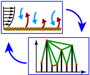
To address this issue, a network-based approach relying on a natural visibility graph (NVG) is employed on a field-experimental dataset in a convective ASL flow (see figure 1(a) for a schematic). The NVG is used since it maps a time series into a network whose features (e.g. network metrics) are sensitive to the temporal structure of the mapped signal (Lacasa et al. Reference Lacasa, Luque, Ballesteros, Luque and Nuno2008) and, therefore, to a specific flow organisation. The NVG has been used for studying different vortical and turbulent flows (Iacobello, Ridolfi & Scarsoglio Reference Iacobello, Ridolfi and Scarsoglio2020), including wall-turbulence (Liu, Zhou & Yuan Reference Liu, Zhou and Yuan2010; Iacobello, Scarsoglio & Ridolfi Reference Iacobello, Scarsoglio and Ridolfi2018; Iacobello, Ridolfi & Scarsoglio Reference Iacobello, Ridolfi and Scarsoglio2021), jets and plumes (Charakopoulos et al. Reference Charakopoulos, Karakasidis, Papanicolaou and Liakopoulos2014; Iacobello et al. Reference Iacobello, Marro, Ridolfi, Salizzoni and Scarsoglio2019), and turbulent combustors (Murugesan & Sujith Reference Murugesan and Sujith2015; Gotoda et al. Reference Gotoda, Kinugawa, Tsujimoto, Domen and Okuno2017). The details of this method and the dataset are described in § 2. The results of the analysis are presented in § 3, where we show through various network metrics that the velocity and temperature signals are characterised by different temporal structures. Finally, in § 4 conclusions are drawn and future research directions are provided.

Figure 1. (a) Schematic of a convective ASL flow set-up (left), and the natural visibility graph (NVG) construction (right) from original and mirrored signals,  $s_i$ and
  $-s_i$, respectively. Panels (b,c) show two examples of signals,
  $s_i$, depicted as vertical blue bars, and the corresponding NVGs: (b) non-intermittent signal, (c) highly intermittent signal. Nodes and links of the networks are depicted as red filled circles and green straight lines, respectively. The degree values,
  $\kappa _i$, for each node
  $i=1,\ldots ,20$ are listed at the bottom. In both panels node
  $i=17$ is highlighted in black and its links in orange. The index,
  $j$, of neighbours of
  $i=17$ and the corresponding degree,
  $\kappa _j$, are also listed in two tables.
2. Methodology and dataset
2.1. Visibility graph and network metrics
In order to capture the changes in the temporal structure of the signals, the NVG approach is employed, where network nodes correspond to temporal instants,  $i=1,\ldots ,N$, of a time series,
  $s(t_i)$, while links are active if a convexity criterion is satisfied (Lacasa et al. Reference Lacasa, Luque, Ballesteros, Luque and Nuno2008). Specifically, two nodes
  $\{ i,j\}$, corresponding to signal values
  $\{ t_i, s(t_i)\}$ and
  $\{ t_j, s(t_j)\}$, are linked with each other if the condition (2.1) is fulfilled for any
  $t_i< t_n< t_j$,
 \begin{equation} s(t_n)< s(t_j)+\left(s(t_i)-s(t_j)\right)\frac{t_j-t_n}{t_j-t_i}. \end{equation}
 For instance, figure 1(b,c) shows two synthetic signals,  $s(t_i)$, and their corresponding visibility networks (depicted as red nodes and green links). The information on the link activation among nodes is then stored in the (binary) adjacency matrix, whose entries
  $A_{i,j}$ are equal to
  $1$ if there is a link between nodes
  $\{ i,j\}$ with
  $i\neq j$, and
  $0$ otherwise (Newman Reference Newman2018). Although the NVG algorithm is typically used as a convexity criterion, it can also be employed as a concavity criterion applying (2.1) to the mirrored signal
  $-s(t)$ (figure 1a).
Visibility graphs represent a class of network-based tools that, owing to its parameter-free nature and simplicity of implementation, has been largely adopted so far for signal analysis (Zou et al. Reference Zou, Donner, Marwan, Donges and Kurths2019). In particular, visibility graphs have shown to be able to inherit the structure of the signal, also accounting for nonlinear effects (Lacasa et al. Reference Lacasa, Luque, Ballesteros, Luque and Nuno2008; Manshour Reference Manshour2015; Manshour, Tabar & Peinke Reference Manshour, Tabar and Peinke2015; Iacobello et al. Reference Iacobello, Ridolfi and Scarsoglio2021). However, as per any other tool for time series analysis, some limiting aspects should be considered when visibility graphs are employed, such as the choice of the sampling frequency or the series length (Donner & Donges Reference Donner and Donges2012). Specifically, sampling frequency should be sufficiently high to capture the smallest scales of interest, while the signal length should be sufficiently long to capture the largest (temporal) scales. Recently, Iacobello et al. (Reference Iacobello, Ridolfi and Scarsoglio2021) also evaluated the effect of high-frequency noise on experimental data on the visibility graph analysis of large-to-small scale frequency modulation in wall-bounded turbulence, showing a good robustness of the method. Finally, we note that the NVGs are insensitive to affine transformations of the signal, namely to shifting and rescaling operation on the series axes (Lacasa et al. Reference Lacasa, Luque, Ballesteros, Luque and Nuno2008), as a consequence of the linearity of the right-hand side of inequality (2.1).
In order to characterise a network structure, and in turn the mapped signal, a set of network metrics have to be selected. One of the simplest metrics is the degree centrality,  $\kappa _i$, defined as the number of neighbours of
  $i$, i.e. the nodes linked to
  $i$ (Newman Reference Newman2018). As shown in figure 1(b,c), the presence of locally convex intervals leads to the appearance of high-degree (i.e. highly connected) nodes, which are typically associated with peaks in the signal. A point of a time series is here said to be a peak if it is a local (or global) maximum of the signal (Iacobello et al. Reference Iacobello, Scarsoglio and Ridolfi2018), namely its magnitude is comparable with the maximum excursion of the series (i.e. the difference between the maximum and the minimum values). A pit is the counterpart of a peak, namely a local (or global) minimum of the signal. Therefore, as network metrics (e.g. the degree centrality) are employed to characterise the signals’ temporal structure, the ratio of the metrics for both NVG variants (i.e. built on the original and mirrored signals) can be used to study peaks-pits asymmetry in the signals (Hasson et al. Reference Hasson, Iacovacci, Davis, Flanagan, Tagliazucchi, Laufs and Lacasa2018). In particular, the presence of peak-pit asymmetry in quantities (e.g. velocity and temperature) characterising a flow field, physically represents the tendency of the flow to display strong positive or negative fluctuations (Iacobello et al. Reference Iacobello, Marro, Ridolfi, Salizzoni and Scarsoglio2019).
With the aim to quantify large-scale intermittency, the assortativity coefficient,  $r$, is employed. Here
  $r$ is defined as the Pearson correlation coefficient between the degree of the nodes at the ends of each link, namely
  $r= \text {cov}[\kappa _i,\kappa _j]/ (\sigma [\kappa _i] \sigma [\kappa _j])$,
  $\forall i,j$ so that
  ${A_{i,j}=1}$ (Newman Reference Newman2018). Here,
  $\text {cov}[\bullet ,\bullet ]$ and
  $\sigma [\bullet ]$ are the covariance and standard deviation, respectively. For example, in figure 1(b,c) the indices,
  $j$, of the neighbours of representative node
  $i=17$ are listed together with the corresponding degree values,
  $\kappa _j$. In figure 1(b),
  $\kappa _j$ values are similar to
  $\kappa _i=6$, while in figure 1(c),
  $\kappa _j$ values are dissimilar to
  $\kappa _i=9$. In the former case, nodes tend to link with other similar nodes so the
  $r$ value tends to increase (toward positive values); in the latter case, instead, nodes tend to link with other dissimilar nodes so the
  $r$ value tends to decrease (towards negative values).
Iacobello et al. (Reference Iacobello, Marro, Ridolfi, Salizzoni and Scarsoglio2019) showed that  $r$ is an effective metric in quantifying intermittency in experimental signals of a meandering passive-scalar plume. Figure 1(c) shows an example of the temporal structure of an intermittent signal (conceptual diagram). This structure can be compared with a not-so intermittent signal (figure 1b), where the subsequent values of the signal are closer to each other. In figure 1(c) peaks correspond to network hubs (high
  $\kappa$), which are mostly linked to nodes with lower degree values. Therefore, for intermittent signals, the corresponding NVGs tend to show smaller
  $r$ values tending towards negative values. In general, lower
  $r$ values correspond to the strongest intermittent behaviours in the signal (Iacobello et al. Reference Iacobello, Marro, Ridolfi, Salizzoni and Scarsoglio2019). Contrarily, low degrees of intermittency can be linked to higher and often positive values of
  $r$, as in figure 1(b). Accordingly, the asymmetry between the intermittent behaviour of peaks and pits can be captured by evaluating the assortativity values of visibility graphs built from the original signals,
  $r$, and mirrored signals,
  $r_M$.
2.2. Dataset description
We applied NVG on the dataset from the surface layer turbulence and environmental science test (SLTEST) experiment, which was conducted over a homogeneous and flat terrain at the Great Salt Lake desert in Utah, USA (40.14 $^\circ$ N, 113.5
 $^\circ$ W). The experiment ran continuously for nine days from 26 May 2005 to 03 June 2005. In this experiment nine time-synchronised sonic anemometers (CSAT3, Campbell Scientific, Logan, USA) were mounted on a 30 m mast at heights
  $z=\{$1.4, 2.1, 3, 4.3, 6.1, 8.7, 12.5, 17.9, 25.7
 $\}$ m, levelled to within
  $\pm$0.5
 $^\circ$ from the true vertical. Note that the lowest measurement height (
 $z=$ 1.4 m) at the SLTEST site was more than three orders of magnitude larger than the aerodynamic roughness length, which was
  $z_{0}\approx$5 mm (Metzger, McKeon & Holmes Reference Metzger, McKeon and Holmes2007). Each of these nine anemometers measured the three wind components and sonic temperature at a sampling frequency of 20 Hz. Other details of the set-up and the instruments can be found in previous works (e.g. Hutchins & Marusic Reference Hutchins and Marusic2007; Chowdhuri, Kumar & Banerjee Reference Chowdhuri, Kumar and Banerjee2020).
In a convective ASL flow the standard practice is to compute the turbulent statistics over a 30 min period (Panosfsky & Dutton Reference Panosfsky and Dutton1984; Kaimal & Finnigan Reference Kaimal and Finnigan1994). Accordingly, the data from all the nine sonic anemometers were divided into 30 min segments, with each segment containing the 20 Hz measurements of the three wind components and the sonic temperature. Thereafter, we rotated the coordinate systems of all the nine sonic anemometers in the streamwise direction by applying the double-rotation method of Kaimal & Finnigan (Reference Kaimal and Finnigan1994) for each 30 min period. The turbulent fluctuations in the wind components ( $u^{\prime }$,
  $v^{\prime }$ and
  $w^{\prime }$ in the streamwise, cross-stream and vertical directions, respectively) and in the sonic temperature (
 $T^{\prime }$) were calculated after removing the 30 min linear trend from the associated variables. To select the 30 min periods for the NVG analysis, we focused only on rain-free daytime convective periods and followed the detailed data selection methods as outlined in Chowdhuri et al. (Reference Chowdhuri, Kumar and Banerjee2020).
In ASL flows, when turbulence is primarily dominated by buoyancy or shear, the time-averaged momentum or heat flux values become small (i.e. tend to zero). Although the vertical profiles of the heat and momentum fluxes in such flows should be constant with height (Panosfsky & Dutton Reference Panosfsky and Dutton1984), due to the smallness of the flux values, vertical variations in the flux profiles are often noticed (Stiperski & Calaf Reference Stiperski and Calaf2018; Chowdhuri, McNaughton & Prabha Reference Chowdhuri, McNaughton and Prabha2019). Therefore, to include enough data that span from buoyancy-dominated to shear-dominated turbulence, we selected 30 min periods with at most a 40 % vertical variation in the heat and momentum fluxes with respect to the corresponding flux values at the lowest  $z$. As a result, for all the selected 30 min periods from the convective conditions, a total of 1224 time series were collected in the range
  $10^{-3}<-\zeta <10^2$, where
  $-\zeta =z/L$ is the stability parameter,
  $z$ is the measurement height and
  $L$ is the Obukhov length. Since
  $L$ is the height where the turbulence production due to buoyancy equals the production due to shear,
  $-\zeta >1$ denotes ASL flows that are largely dominated by buoyancy (highly convective conditions). On the other hand,
  $-\zeta <0.1$ values conventionally indicate that the ASL flows are mostly dominated by shear (near-neutral conditions).
3. Results
This section reports the results of visibility networks related to the streamwise and vertical velocity fluctuations ( $u^{\prime }$ and
  $w^{\prime }$) and temperature fluctuations (
 $T^{\prime }$) in a convective ASL flow. Note that here
  $\bullet ^\prime$ notation indicates temporal fluctuations, i.e. the variables after the 30 min linear trend is removed. These three variables are chosen since they constitute the turbulent momentum and heat fluxes (
 $u^{\prime }w^{\prime }$ and
  $w^{\prime }T^{\prime }$) and, hence, are important quantities in the ASL turbulence dynamics.
3.1. Intermittency via network assortativity
In order to characterise the statistical features of large-scale intermittency, we begin by investigating the p.d.f.-based higher-order moments of the analysed signals. Figure 2(a,b) shows the skewness ( $\mathcal {S}$) and kurtosis (
 $\mathcal {K}$) of the
  $u^{\prime }$,
  $w^{\prime }$ and
  $T^{\prime }$ signals against the stability ratio
  $-\zeta$. For the
  $T^{\prime }$ signals,
  $\mathcal {S}$ and
  $\mathcal {K}$ significantly exceed their Gaussian values (0 and 3, respectively) for the highly convective conditions (
 $-\zeta >1$). Whereas, in the near-neutral regime (
 $-\zeta <0.1$) the
  $T^{\prime }$ signals remain almost Gaussian. On the other hand, for the
  $u^{\prime }$ signals, the
  $\mathcal {S}$ and
  $\mathcal {K}$ values are very close to their Gaussian counterparts irrespective of stability. However, for the
  $w^{\prime }$ signals, a slight deviation from Gaussianity is observed as compared with the
  $u^{\prime }$ signals.

Figure 2. (a) Skewness,  $\mathcal {S}$, and (b) kurtosis,
  $\mathcal {K}$, of
  $u^{\prime }$,
  $w^{\prime }$ and
  $T^{\prime }$ against the stability parameter,
  $-\zeta$. In (c) the p.d.f.,
  $p(\hat {T})$, of the normalised temperature fluctuations,
  $\hat {T}=T^{\prime }/\sigma _{T}$ (where
  $\sigma _{T}$ is the standard deviation of
  $T^{\prime }$), are shown for the three stability classes (SC): SC1,
  $0<-\zeta <0.1$; SC3,
  $0.3<-\zeta <0.5$; SC6,
  $-\zeta >2$. The solid black line corresponds to the standard Gaussian distribution. (d) Assortativity coefficient,
  $r$, from the
  $u^{\prime }$,
  $w^{\prime }$ and
  $T^{\prime }$ signals against
  $-\zeta$. The green line indicates the
  $r$ values for a Gaussian white noise (GWN). In (e,f) the ratios between
  $r$ from the original
  $u^{\prime }$,
  $w^{\prime }$ and
  $T^{\prime }$ signals and their mirrored (
 $r_{M}$) and shuffled (
 $r_{S}$) counterparts, respectively, are shown.
The near-Gaussian behaviour of the  $u^{\prime }$ and
  $w^{\prime }$ signals suggest that the velocity fluctuations are characterised by a low degree of large-scale intermittency, which agrees with previous studies (e.g. Chu et al. Reference Chu, Parlange, Katul and Albertson1996). But, in the buoyancy-dominated regime (
 $-\zeta >1$), the large skewness and kurtosis of the temperature signals inform that there are intermittent bursts of large positive values amidst the frequent occurrences of small negative fluctuations. To confirm this further, in figure 2(c) we show the temperature p.d.f.s for the three representative stability classes. We notice that at
  $-\zeta >2$, the
  $T^{\prime }$ p.d.f. significantly differs from a Gaussian distribution with anomalous occurrences of large positive
  $T^{\prime }$ values.
Despite the fact that p.d.f.-based analyses of large-scale intermittency have been widely used, they cannot fully explain the role of flow organisation on the signal's intermittent characteristics (Tsinober Reference Tsinober2014). Contrarily, the assortativity coefficient,  $r$, quantifies large-scale intermittency by retaining information on the temporal structure of the signals. In figure 2(d) the behaviour of
  $r$ is shown for the
  $u^{\prime }$,
  $w^{\prime }$ and
  $T^{\prime }$ signals against
  $-\zeta$. For
  $T^{\prime }$, the
  $r$ values undergo a gradual transition between two distinct plateaus of constant values for the near-neutral (
 $-\zeta <0.1$) and highly convective (
 $-\zeta >1$) conditions. Particularly, in the near-neutral regime the
  $r$ values of
  $T^{\prime }$ remain close to a Gaussian white noise. Since a decrease in
  $r$ is sensitive to an increasing large-scale intermittency of the signal, the temperature fluctuations in a buoyancy-dominated ASL flow (
 $-\zeta >1$) appear more intermittent as compared with a shear-dominated ASL flow (
 $-\zeta <0.1$). We also observe that
  $r$ remains almost invariant with
  $-\zeta$ for
  $w^{\prime }$, while a slight increase in
  $r$ is observed for
  $u^{\prime }$.
The similarity between  $r$ and p.d.f.-based statistics as a function of
  $-\zeta$ validates our metric, which is able to capture the main features of the underlying dynamics. On this note, the NVGs can be further used to assess whether the large-scale intermittency in the signal is related to the positive or negative fluctuations via studying the assortativity coefficients of the original (
 $r$) and mirrored (
 $r_{M}$) signals. Figure 2(e) shows the ratio
  $r/r_{M}$ that characterises the asymmetry in large-scale intermittency between positive and negative fluctuations from a network perspective. For
  $T^{\prime }$ signals,
  $r/r_{M}$ decreases from the shear-dominated regime towards the buoyancy-dominated regime. Physically this indicates that, for highly convective regimes (
 $-\zeta >1$), the mirrored signal is less intermittent, given that
  $r_{M}>r$ (see figure S1 in the supplementary material available at https://doi.org/10.1017/jfm.2021.720). Moreover, since the changes in
  $r_{M}$ with
  $-\zeta$ remain significantly less as compared with
  $r$ (see figure S1), the behaviour of
  $r/r_{M}$ tends to mimic the behaviour of
  $r$. Therefore, in highly convective conditions the large-scale intermittency in
  $T^{\prime }$ is dictated by positive fluctuations (i.e. peaks,
  $T^{\prime }>0$) rather than the negative ones (i.e. pits,
  $T^{\prime }<0$). This finding is consistent with the fact that the p.d.f.s of
  $T^{\prime }$ in the highly convective conditions show a heavy tail towards the positive fluctuations, as evident from figure 2(c). Moreover, the ratio
  $r/r_{M}$ for the two velocity components remains almost constant and approximately equal to 1, suggesting a peak-pit symmetry of the signals for any
  $-\zeta$ in agreement with results shown in figure 2(a,b). It is worth remarking that, despite the aforementioned overall agreement, the NVGs are able to isolate the intermittent behaviour of positive and negative fluctuations, while higher-order moments do not distinguish extreme events as peaks and pits. For instance, the kurtosis (or any other even-order moment) does not distinguish between the positive and negative extreme events, while the skewness does not account for only extreme events but both small and large values in the signal.
To further explore the role of the temporal structure of the signals on large-scale intermittency, we computed the ratios of  $r$ values between the original and randomly shuffled signals,
  $r/r_{S}$. To compute
  $r_{S}$, one shuffled surrogate series was generated for each time series of
  $u^{\prime }$,
  $w^{\prime }$ and
  $T^{\prime }$; however, a larger number of surrogates do not lead to significant changes in
  $r_{S}$. Since random shuffling destroys the temporal dependencies while preserving the signal p.d.f. (and, therefore, all the p.d.f. moments), the deviation from 1 in
  $r/r_{S}$ is an indication of how strong is the impact of the temporal structure on large-scale intermittency. Figure 2(f) illustrates that
  $r/r_{S}$ significantly decreases for
  $T^{\prime }$ and increases for
  $u^{\prime }$ towards
  $-\zeta >1$, while no discernible change is observed for
  $w^{\prime }$. It is thus apparent that, in the buoyancy-dominated regime, the flow organisation plays an important role to determine the temporal arrangement of
  $u^{\prime }$ and
  $T^{\prime }$ values in the signals. However, since shuffling destroys any dependencies in a time series, a more detailed analysis is required to shed light on the relative contribution of linear and nonlinear effects undergoing in the flow, which impact the signal's intermittent features.
3.2. Role of nonlinearity on convective dynamics
To investigate the role of nonlinearity, first we investigate the behaviour of the degree distribution (i.e. the probability to find a node with a given degree value,  $\kappa$), since it is strongly related to the temporal structure of the mapped signals (Lacasa et al. Reference Lacasa, Luque, Ballesteros, Luque and Nuno2008; Liu et al. Reference Liu, Zhou and Yuan2010). In fact, the degree distribution from the NVG is sensitive to the signal's p.d.f. and on the linear and nonlinear dependencies in the signals (Manshour Reference Manshour2015; Iacobello et al. Reference Iacobello, Scarsoglio and Ridolfi2018). To account for the linear and nonlinear effects, we evaluated the degree distributions of
  $u^{\prime }$,
  $w^{\prime }$ and
  $T^{\prime }$ from two different types of surrogate signals: (i) random shuffling, and (ii) iteratively adjusted amplitude Fourier transform (IAAFT). In the IAAFT method, surrogate data are generated that do not contain nonlinear effects but preserve the linear effects described by the auto-correlation in the time series (Lancaster et al. Reference Lancaster, Iatsenko, Pidde, Ticcinelli and Stefanovska2018). To achieve such an objective, the Fourier amplitudes of the time series are kept intact (thereby preserving the auto-correlation), but the associated Fourier phases are replaced by a random uniform distribution between 0 to 2
 ${\rm \pi}$. The randomness in the Fourier phases destroys any nonlinear structure of the time series. However, due to the randomisation of the Fourier phases the p.d.f. of the time series is altered to be Gaussian. Hence, to preserve both the p.d.f. and amplitude spectrum, the Fourier amplitudes and the signal's p.d.f.s are adjusted iteratively at each stage of phase randomisation until the resultant signal has the same power spectrum and p.d.f. as the original one. Lancaster et al. (Reference Lancaster, Iatsenko, Pidde, Ticcinelli and Stefanovska2018) provides a step-by-step implementation of the IAAFT algorithm, which has also been applied to turbulence studies (Poggi et al. Reference Poggi, Porporato, Ridolfi, Albertson and Katul2004; Basu et al. Reference Basu, Foufoula-Georgiou, Lashermes and Arnéodo2007; Cabrit, Mathis & Marusic Reference Cabrit, Mathis and Marusic2013; Keylock Reference Keylock2017).
In figure 3(a–c) we show the complementary cumulative distribution functions (CCDFs) of the degree,  $1-P(\kappa )$ (where
  $P(\kappa )$ is the degree CDF), from the original, shuffled and IAAFT surrogates of
  $u^{\prime }$,
  $w^{\prime }$ and
  $T^{\prime }$, for three representative stability classes (see Appendix for CCDFs of
  $\kappa$ from all the six stability classes). Complementary cumulative distribution functions are typically used to overcome the intrinsically fat-tailed behaviour of degree distributions and to highlight the contribution from high
  $\kappa$ values (Newman Reference Newman2018). Irrespective of the stability class, the CCDFs of original signals (orange lines) and their randomly shuffled surrogates (blue lines) remain far apart from each other, revealing the strong effect of the signal's temporal structure on the network topology (Iacobello et al. Reference Iacobello, Scarsoglio and Ridolfi2018). On the other hand, the difference between the CCDFs from original and IAAFT signals (green lines in figure 3a–c) are less evident. Only for temperature,
  $T^{\prime }$, a remarkable difference in CCDFs is observed in the highly convective regime (figure 3c), which systematically disappears as the near-neutral regime is approached (figure 3a).

Figure 3. The CCDFs,  $1-P(\kappa )$, of the degree,
  $\kappa$, from the original, shuffled and IAAFT signals corresponding to three representative stability classes (SC): (a)
  $0<-\zeta <0.1$, (b)
  $0.3<-\zeta <0.5$ and (c)
  $-\zeta >2$. For clarity purposes, the distributions are shifted vertically by five and ten decades for
  $w^{\prime }$ and
  $u^{\prime }$, respectively. (d) The L1-norm,
  $\mathcal {L}_{log}$, between the difference of original and IAAFT signals for the six SC. (e) Ratio,
  $r/r_{I}$, against
  $-\zeta$ between
  $r$ from the original signals and
  $r_{I}$ from the IAAFT signals. For comparison, the ratio
  $r/r_{S}$ of the
  $T^{\prime }$ signal (figure 2f) is included in (e) as a green line.
The comparison between the original degree distributions and their IAAFT surrogates is useful to assess the net role of nonlinearity on the signal's temporal structure, since these surrogates retain only the signal's p.d.f. and its linear correlations. Therefore, the results of figure 3(a–c) suggests that the effects of nonlinearity remain quite different on the temporal structure of velocity and temperature fluctuations, despite being part of the same nonlinear system (i.e. atmospheric turbulence at a large Reynolds number). In order to quantify the net effect of nonlinearity in  $P(\kappa )$, we calculated the L1-norm of the difference between the logarithms of
  $P(\kappa )$, i.e.
  $\mathcal {L}_{\log }=\|\log [P(\kappa )_{{I}}]-\log [P(\kappa )_{{O}}] \|_1$, where
  $I$ and
  $O$ subscripts refer to IAAFT and original signals, respectively. The L1-norm is a simple yet useful metric to compare the difference between two probability distributions (Hasson et al. Reference Hasson, Iacovacci, Davis, Flanagan, Tagliazucchi, Laufs and Lacasa2018). The logarithm is taken since
  $P(\kappa )$ have an exponential tail so that in computing the L1-norm we balance the contribution to
  $P(\kappa )$ coming from low and high
  $\kappa$ values.
In figure 3(d) we present the  $\mathcal {L}_{\log }$ values between the original and IAAFT signals as a bar plot for the same six stability classes. In the near-neutral regime (
 $0<-\zeta <0.1$) the impact of nonlinearity is rather low and similar for all the signals. For the
  $T^{\prime }$ signals, the
  $\mathcal {L}_{\log }$ values gradually increase as the highly convective regime (
 $-\zeta >2$) is approached. This implies that the temporal structure of the temperature fluctuations becomes highly sensitive to the nonlinear dependencies in such conditions. On the other hand, for the velocity signals, we observe that the L1-norm for the
  $w^{\prime }$ signals is slightly larger than the
  $u^{\prime }$ signals. This outcome suggests that the
  $w^{\prime }$ signals appear more affected than the
  $u^{\prime }$ signals by nonlinear dependencies for large
  $-\zeta$ values.
So far, we have reported through the degree distribution that the NVGs not only are sensitive to the full temporal structure (figure 3a–c), but are also able to highlight the impact of nonlinear dependencies in the signals (figure 3d). Therefore, since the NVG changes with nonlinearity, the network assortativity coefficient,  $r$, – which accounts for signal intermittency – is also expected to change. To evaluate such a variation in
  $r$, figure 3(e) illustrates the ratio,
  $r/r_{I}$, computed between
  $r$ for the original signals, and
  $r_I$ for its IAAFT surrogates. Note that, in accordance with Poggi et al. (Reference Poggi, Porporato, Ridolfi, Albertson and Katul2004), we used 10 IAAFT surrogates for each signal to compute the
  $r_I$ values. Values of
  $r/r_{I}$ close to 1 indicate that there is a negligible impact of nonlinearity on the signal intermittency, since
  $r$ accounts for both linear and nonlinear effects, while
  $r_{I}$ only for linear effects. For the
  $T^{\prime }$ signals,
  $r/r_{I}$ decreases from 1 in the shear-dominated regime to around 0.6 in the buoyancy-dominated regime. Interestingly,
  $r/r_I$ for the
  $T^{\prime }$ signals is almost coincident with the corresponding
  $r/r_S$ (green line in figure 3e), which accounts for both linear and nonlinear effects on the signal's temporal structure. Hence, it indicates that the temperature intermittency – especially in the highly convective regime – is mainly characterised by the nonlinear dependencies in the signal, while the linear effects are negligible.
Contrarily, for the velocity signals, the effect of nonlinearity on  $r$ is different. For
  $u^{\prime }$ signals, the ratio
  $r/r_{I}$ remains almost constant with
  $-\zeta$ (figure 3e), although its
  $r/r_{S}$ values increase with
  $-\zeta$ (figure 2f). This suggests that the changes in the temporal structure of
  $u^{\prime }$ are primarily governed by linear dependencies – described by the amplitude spectrum – as the highly convective regime is approached. For the ASL flows, it is known that there is an increase in large-scale spectral energy with respect to the small scales, as the turbulence production due to buoyancy is increased (Wyngaard Reference Wyngaard2010). This relative increase in large-scale spectral energy results in smoother
  $u^{\prime }$ signals, given the small scales are less energetic. In general, smoother signals correspond to more regular NVGs and higher assortativity values (Iacobello et al. Reference Iacobello, Scarsoglio and Ridolfi2018, Reference Iacobello, Marro, Ridolfi, Salizzoni and Scarsoglio2019, Reference Iacobello, Ridolfi and Scarsoglio2021). Thus, the increasing trend shown in figure 2(f) for
  $u^{\prime }$ is mainly related to linear effects and is a result of a change in the spectral energy at small and large scales. For
  $w^{\prime }$, on the other hand, we see that the ratio
  $r/r_I$ decreases in the highly convective regime. Similar to
  $u^{\prime }$, as the convective regime is approached, the large-scale spectral energy increases with respect to the small scales (Wyngaard Reference Wyngaard2010), thus making the
  $w^{\prime }$ signal smoother. Linear effects, therefore, would make the assortativity increase while (as shown in figure 3e) nonlinear effects make it decrease. The net effect is an apparent independence of the assortativity on the full temporal structure with
  $-\zeta$, as clearly observed in figure 2(f). In other words, there is a balance between the linear and nonlinear effects which govern the temporal structure of the
  $w^{\prime }$ signals in the buoyancy-dominated regime.
4. Discussion and conclusions
The impact of the temporal structure – including both linear and nonlinear dependencies – on large-scale intermittency in convective ASL flows is addressed for the first time through a visibility graph approach. The stability conditions have the strongest impact on the temporal structure of the  $T^{\prime }$ signals, while their impact is weaker on the temporal structure of the
  $u^{\prime }$ and
  $w^{\prime }$ signals. Combining visibility graphs and surrogate data, we demonstrate that the intermittent structure of
  $T^{\prime }$ in convective conditions is associated with strong nonlinear dependencies in the signal. In fact, in highly convective ASL flows, the small negative fluctuations observed in
  $T^{\prime }$ are a signature of the cold downdrafts, which bring well-mixed air from aloft (the upper regions of the ASL flow or the mixed layer, see figure 1a) to the heights closer to the ground. On the other hand, the large positive temperature fluctuations can be related to warm updrafts associated with the hot plumes rising from the surface. Therefore, the observed intermittency in temperature could be due to a complex nonlinear interaction between the cold downdrafts and warm updrafts, which results in a specific temporal pattern that appears to be intermittent. Put differently, in highly convective ASL flows, a nonlinear interplay between the temperature field and the underlying turbulent flow dynamics seems to be responsible for the large-scale intermittency in the temperature fluctuations.
As discussed in his seminal work, Batchelor (Reference Batchelor1953) observed that the nonlinear terms in the governing equations of turbulence would influence the non-Gaussian behaviour of the velocity increments, i.e. the small-scale intermittency. Recently, Zorzetto, Bragg & Katul (Reference Zorzetto, Bragg and Katul2018) confirmed the nonlinear character of the system is responsible for the small-scale intermittency in the statistics of temperature increments. However, our results illustrate that the nonlinearity even affects the non-Gaussian characteristics of the single-point measurements of temperature fluctuations in highly convective conditions (i.e. large-scale intermittency). This finding is not trivial because it implies that, for temperature fluctuations, the nonlinear effects even persist at scales comparable to the energy-containing scales of motions that cause the highly energetic activities in  $T^{\prime }$, thus leading it to be non-Gaussian (Majda & Kramer Reference Majda and Kramer1999). Hence, it can be inferred that, since the nonlinearity influences both the small- and large-scale intermittency in temperature fluctuations, these two phenomena seem to be coupled in the case of temperature signals.
Although it currently represents a conjecture, some experimental evidence exists that supports this picture. For instance, in Rayleigh–Bénard convection experiments it has been found that the non-Gaussian statistics of temperature increments (statistics of temperature derivatives and dissipation rate) and temperature fluctuations are closely linked together (Belmonte & Libchaber Reference Belmonte and Libchaber1996; Emran & Schumacher Reference Emran and Schumacher2008). Similarly, in a highly convective ASL flow the ramp-cliff structures (slow rises followed by a sudden drop) in the  $T^{\prime }$ time series have been found to affect the small-scale and large-scale intermittency in such signals. In fact, while ramp-cliff structures are a signature of the presence of convective plumes inducing non-Gaussian temperature p.d.f.s (Chu et al. Reference Chu, Parlange, Katul and Albertson1996), thus contributing to large-scale intermittency, they have also been shown to impact the small-scale intermittency of temperature during highly convective conditions (Zorzetto et al. Reference Zorzetto, Bragg and Katul2018).
Concerning velocity fluctuations, with the change in the stability ratio ( $-\zeta$), the linear effects (related to the Fourier spectra) play a stronger role in determining the temporal structure of the
  $u^{\prime }$ and
  $w^{\prime }$ signals than
  $T^{\prime }$. Specifically, the change in the temporal structure of
  $u^\prime$ with stability is driven by a relative increase and decrease in the spectral energy at large and small scales, respectively. This leads
  $u^{\prime }$ signals to be less intermittent than temperature signals, as revealed by higher assortativity values. On the other hand, a competition between the linear and nonlinear effects inhibits temperature-like intermittency in the
  $w^{\prime }$ signals.
The results provided in this study represent a first attempt towards advancing the level of information of p.d.f.-based analyses, thus fostering the possibility to improve the understanding of large-scale intermittency in convective ASL flows, a seldom-explored topic in the literature. More importantly, complex networks can be a powerful tool to assess the role of nonlinearity on the organisation of coherent structures, and its impact on the turbulent fluxes. On this note, to further shed light on how the organised structures in a convective ASL flow affect the intermittent features of the heat and momentum flux signals, an explicit assessment of the inter-relations between the velocity and temperature signals would be required. This should also involve more advanced analyses, e.g. via multi-layer networks (Kivelä et al. Reference Kivelä, Arenas, Barthelemy, Gleeson, Moreno and Porter2014), whose application is out of the scope of the present manuscript and will be the subject of a future research. In conclusion, based on current findings and methodology, we do believe the present work could open up new research avenues in studying large-scale intermittency in convective flows.
Supplementary material
Supplementary material is available at https://doi.org/10.1017/jfm.2021.720.
Acknowledgements
S.C. is indebted to Dr K.G. McNaughton for providing the SLTEST dataset. S.C. also acknowledges the Director of IITM and Dr T. Prabhakaran for their constant encouragement.
Funding
The Indian Institute of Tropical Meteorology (IITM) is an autonomous institute fully funded by the Ministry of Earth Sciences, Government of India. T.B. acknowledges the funding support from the University of California Laboratory Fees Research Program funded by the UC Office of the President (UCOP), grant ID LFR-20-653572. Additional support was provided to T.B. by the new faculty start up grant provided by the Department of Civil and Environmental Engineering, and the Henry Samueli School of Engineering, University of California, Irvine.
Declaration of interests
The authors report no conflict of interest.
Author contributions
S.C. and G.I. designed the study and carried out the analyses. G.I. prepared the figures and S.C. wrote the initial draft of the manuscript. G.I. and T.B. provided their corrections, comments and suggestions. All the authors read the final draft and agreed to all the changes.
Appendix. Degree distributions for all stability classes
In this appendix the behaviour of the CCDFs of the degree,  $\kappa$, for six different stability classes is reported. This is to highlight the change in the overall temporal structure of the
  $u^{\prime }$,
  $w^{\prime }$ and
  $T^{\prime }$ signals as the ASL transitions from the buoyancy- to shear-dominated regime. The CCDFs are illustrated in figure 4 in a log-linear plot for the three variables, showing exponential tails. For the
  $u^{\prime }$ and
  $T^{\prime }$ signals (figure 4a,c), the slopes of the distributions get gradually steeper as
  $-\zeta \rightarrow 0$, i.e. as the ASL approaches the near-neutral conditions. On the contrary, a small change is observed in the slopes of the
  $w^{\prime }$ signals (figure 4b). The results shown in figure 4 are qualitatively in general accordance with the behaviour of
  $r$ as shown in figure 2(d) (which focuses on the intermittent structure of the signals). In fact, in both figures we observe stronger changes with
  $-\zeta$ for the
  $u^{\prime }$ and
  $T^{\prime }$ signals, and weaker variations in
  $w^{\prime }$.

Figure 4. The CCDFs ( $1-P(\kappa )$) of the degrees (
 $\kappa$) are shown for the (a)
  $u^{\prime }$, (b)
  $w^{\prime }$ and (c)
  $T^{\prime }$ signals corresponding to the six stability classes. The classifications of the stability classes according to the ranges in
  $-\zeta$ are in agreement with Liu et al. (Reference Liu, Hu and Cheng2011). Each stability class contains over one hundred 30 min runs, thus ensuring the statistical robustness of the degree distributions presented here.


