


1. Introduction
Understanding the flow properties of concentrated suspensions is a real challenge in the development of many industrial products (e.g. solid propellant rocket motors and fresh concrete) and in the description of various environmental flows (e.g. torrential lava, mud flows and submarine slides). Among other transport properties, shear-induced particle migration has received increasing attention in recent decades. Particle migration can be due to inertial effects (Segre & Silberberg Reference Segre and Silberberg1962) but also occurs at low Reynolds numbers, for instance, in a Poiseuille flow in which the particles tend to migrate towards the centre of the channel (Koh, Hookham & Leal Reference Koh, Hookham and Leal1994; Hampton et al. Reference Hampton, Mammoli, Graham, Tetlow and Altobelli1997; Butler & Bonnecaze Reference Butler and Bonnecaze1999; Snook, Butler & Guazzelli Reference Snook, Butler and Guazzelli2016), in wide-gap Couette flow towards the outer cylinder (Abbott et al. Reference Abbott, Tetlow, Graham, Altobelli, Fukushima, Mondy and Stephens1991; Graham et al. Reference Graham, Altobelli, Fukushima, Mondy and Stephens1991; Chow et al. Reference Chow, Sinton, Iwamiya and Stephens1994; Sarabian et al. Reference Sarabian, Firouznia, Metzger and Hormozi2019) and outward in the cone-and-plate geometry (Chow et al. Reference Chow, Iwayima, Sinton and Leighton1995).
Another typical example of shear-induced migration is viscous resuspension, whereby an initially settled layer of negatively buoyant particles expands vertically when a shear flow is applied. Viscous resuspension was observed for the first time by Gadala-Maria (Reference Gadala-Maria1979) and later explained by Leighton & Acrivos (Reference Leighton and Acrivos1986) and Acrivos, Mauri & Fan (Reference Acrivos, Mauri and Fan1993), who demonstrated that the height of the resuspended particle layer results from the balance between a downward gravitational flux and an upward shear-induced diffusion flux. The authors studied the resuspension of various particles (different sizes and densities) in two different liquids (different viscosities and densities) sheared in a cylindrical Couette device. They measured the height of the resuspended layer of particles,  $h_s$, as a function of the shear rate and showed that the difference between
  $h_s$ and
  $h_0$ (i.e. the initial sediment height) normalized by
  $h_0$ was a function of only the Shields number defined as the ratio between viscous and buoyancy forces
 \begin{equation} \dfrac{h_s-h_0}{h_0}=f(A)\quad \mbox{with}\ A=\dfrac{9}{2}\dfrac{\eta_0 \dot{\gamma}}{\Delta \rho g h_0}, \end{equation}
where  $\dot {\gamma }$ is the shear rate,
  $\Delta \rho$, the density mismatch and
  $\eta _0$, the viscosity of the suspending fluid. Their experimental results were found to be in very good agreement with the diffusive flux model developed by Leighton & Acrivos (Reference Leighton and Acrivos1986). Later, Zarraga, Hill & Leighton (Reference Zarraga, Hill and Leighton2000) revisited the results of Acrivos et al. (Reference Acrivos, Mauri and Fan1993) to determine the particle normal stress in the vorticity direction,
  $\varSigma _{33}^p$, from the height of the resuspended layer of particles by writing the Cauchy momentum balance in the vertical direction
 \begin{equation} \dfrac{\partial \varSigma_{33}^p}{\partial z}=\Delta \rho g \phi. \end{equation}
where g is the acceleration of gravity.
Then, a relation between  $\varSigma _{33}^p$ and the particle volume fraction at the bottom,
  $\phi _0$, is obtained by the integration of (1.2) from the interface between the suspended layer and the clear liquid at the bottom together with the equation of particle number conservation. The relationship between particle normal stress and shear-induced migration (or resuspension) has been the subject of several studies and is still an active area of investigation (Nott & Brady Reference Nott and Brady1994; Mills & Snabre Reference Mills and Snabre1995; Morris & Brady Reference Morris and Brady1998; Morris & Boulay Reference Morris and Boulay1999; Deboeuf et al. Reference Deboeuf, Gauthier, Martin, Yurkovetsky and Morris2009; Lhuillier Reference Lhuillier2009; Nott, Guazzelli & Pouliquen Reference Nott, Guazzelli and Pouliquen2011; Ovarlez & Guazzelli Reference Ovarlez and Guazzelli2013). The suspension balance model proposed by Morris & Boulay (Reference Morris and Boulay1999) and refined by Lhuillier (Reference Lhuillier2009) and Nott et al. (Reference Nott, Guazzelli and Pouliquen2011) offers a promising framework for modelling shear-induced particle migration, but it suffers from a relative lack of experimental data on particle normal stresses.
In addition to the above-cited work of Zarraga et al. (Reference Zarraga, Hill and Leighton2000), who used the viscous resuspension experiment of Acrivos et al. (Reference Acrivos, Mauri and Fan1993) to deduce  $\varSigma _{33}^p$ for particle volume fractions ranging from
  $0.3$ to
  $0.5$, Deboeuf et al. (Reference Deboeuf, Gauthier, Martin, Yurkovetsky and Morris2009) determined
  $\varSigma _{33}^p$ for particle volume fractions ranging from
  $0.3$ to
  $0.5$ through the measurement of the pore pressure in a cylindrical Couette flow. Boyer, Guazzelli & Pouliquen (Reference Boyer, Guazzelli and Pouliquen2011) used a pressure-imposed shear cell to measure
  $\varSigma _{22}^p$ in the range
  $\phi \in [0.4,0.585]$, and Dbouk, Lobry & Lemaire (Reference Dbouk, Lobry and Lemaire2013) determined
  $\varSigma _{22}^p$ in the range
  $\phi \in [0.3,0.47]$ through the measurement of both the total stress
  $\varSigma _{22}$ and the pore pressure. See Guazzelli & Pouliquen (Reference Guazzelli and Pouliquen2018) for a review. All of these studies show a quasi-linear relationship between the particle normal stress components and the shear rate, but recently, Saint-Michel et al. (Reference Saint-Michel, Manneville, Meeker, Ovarlez and Bodiguel2019) performed X-ray radiography experiments on viscous resuspension that revealed a nonlinear relationship with the shear rate.
In this paper, we present the experimental results of viscous resuspension in a Couette device in which the local particle volume fraction and the local shear rate are measured by optical imaging. The value of  $\varSigma _{33}^p$ is obtained by integrating (1.2) from the interface between the clear fluid and the resuspended layer to any height
  $z$ below the interface. These experiments present the dual advantage that
  $\varSigma _{33}^p$ can be determined for a wide range of particle fractions and that the local shear rate can be measured to accurately test the scaling of particle normal stresses with shear rate. In § 2, we present the experimental device and the methods used to compute both the velocity field and the particle concentration field, for Shields numbers ranging from
  $10^{-3}$ to
  $1$. Section 3 is devoted to the results. We first discuss the radial profiles of velocity and of particle concentration. Then we present the vertical concentration profiles from which
  $\varSigma _{33}^p$ is deduced. We finish with some concluding remarks (§ 4).
2. Materials and methods
2.1. Suspension and device
Polymethacrylate (PMMA) spheres (Arkema BS572),  $2a=268\pm 25\ \mathrm {\mu } \textrm {m}$ in diameter and
  $1.19\times 10^{3}\pm 10\ \textrm {kg}\ \textrm {m}^{-3}$ in density, are used. The particles are dispersed in Triton X 100 to which a small amount of a fluorescent dye (Nile Blue A, Sigma-Aldrich) is added. This mixture is Newtonian with a viscosity of
  $\eta _0=0.34 \pm 0.02\ \textrm {Pa}\ \textrm {s}$ and a density
  $1.06\times 10^3\pm 10\ \textrm {kg}\ \textrm {m}^{-3}$ at
  $T=23\,^\circ \textrm {C}$. The characteristic settling velocity of the particles is then
  $V_S= 2/9 \Delta \rho g/ a^2\eta \approx 20\ \mathrm {\mu } \textrm {m}\ \textrm {s}^{-1}$. The liquid and the particles are chosen to have roughly the same refractive index,
  $1.49$, and accurate index matching is achieved by tuning the temperature of the chamber that contains the rheometer.
The resuspension experiments are conducted in a Couette cell made of PMMA mounted on a controlled-stress rheometer (Mars II, Thermofisher) (see figure 1a). The rotor has a radius  $R_1 = 19\ \textrm {mm}$, and the stator has a radius
  $R_2 = 24\ \textrm {mm}$. Thus, the gap is much larger than the particle diameter (
 $(R_2-R_1)/a \approx 37$) and the variation of the shear stress over the gap is expected to be of the order of 1.6 (
 $\varSigma _{12}(R_1)/\varSigma _{12}(R_2)=R_2^2/R_1^2\approx 1.6$). The impact of the stress variation on particle migration will be discussed in § 3.1.

Figure 1. (a) Sketch of the experimental device. (b) View from above. The vertical laser sheet is shifted by an offset of length  $y_0<R_1$ from the radial position (dashed line);
  $x$ is the horizontal position in the laser sheet, and
  $z$ is the vertical position;
  $z=0$ is set by the mercury/suspension interface.
The bottom of the Couette cell is filled with mercury to prevent the particles from migrating out of the gap (under the cup) and to maximize slip at the suspension/bottom interface in order to have a shear rate as homogeneous as possible inside the gap. The suspension is poured into the rheometer cell and illuminated by a thin vertical laser sheet (thickness  ${\approx }50\ \mathrm {\mu } \textrm {m}$) offset by
  $y_0=16.2\ \textrm {mm}$ from the radial plane (see figure 1b). A camera (IDS, nominal frequency 33 Hz, full resolution
  $4104 \times 2174 \ \textrm {px}^2$) is placed at
  $90^\circ$ to the enlightened plane. The accurate matching of the refractive index, the thinness of the laser sheet and the resolution of the camera allow the recording of high-quality images with a resolution of 30 px per particle.
2.2. Experimental procedure and measurement method
2.2.1. Experimental procedure
In this paper, we will focus on the steady state of resuspension obtained for various angular velocities of the rotor,  $\varOmega$:
  $0.3$, 0.5, 1, 2, 5, 10, 20, 30, 40 and 60 rotations per minute (r.p.m.). For all these angular velocity values, the Reynolds number and the Taylor number are less than
  $1$ (for the highest angular velocity,
  $\mathcal {R}e= \rho \varOmega R_1(R_2-R_1)/\eta \approx 1$ and
  $Ta=4 \rho ^2 \varOmega ^2(R_2-R_1)^4/\eta ^2 \approx 1$) and the Péclet number is very large (
 $\mathcal {P}e=6{\rm \pi} \eta a^3\dot {\gamma }/k_B T >10^{8}$, with
  $k_B$ the Boltzmann constant). Note that the inertial effects have also to be compared with the gravity forces. The ratio of inertial to gravitational forces can be written as
  $R_i\varOmega ^2/g$. In our experiment this number is comprised between
  $10^{-6}$ and
  $10^{-1}$, meaning that inertial effects can indeed be neglected. Furthermore, beyond this simple evaluation, Saint-Michel et al. (Reference Saint-Michel, Manneville, Meeker, Ovarlez and Bodiguel2019) performed two-dimensional calculations to evaluate the role of the centrifugal forces that arise due to geometry curvature and showed that inertia effects do not alter the concentration profiles for
  $R_i\varOmega ^2/g<1$.
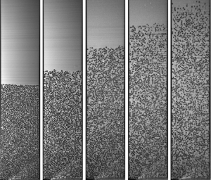
To reach the steady state, the suspension is first sheared with an angular velocity of the rotor equal to 5 r.p.m. for one hour. Then, the speed is set to the desired value for a period until the steady state is reached; the steady state is considered attained when the torque applied by the rheometer becomes constant. The time duration necessary to achieve the steady state is approximately a few hours. Figure 2 shows the viscous resuspension observed for a few rotor angular velocity values. As  $\varOmega$ increases, the resuspended height increases and the bulk particle concentration decreases.

Figure 2. (a) Typical images recorded for different rotor rotation speeds. A photo of the settled layer ( $\varOmega =0$) is also presented (height 21.3 mm). (b) Mapping of the particle volume fraction averaged over 10 000 images (with the exception of the sediment for which only
  $20$ images have been used). (c) Azimuthal velocity normalized by the rotor velocity
  $\varOmega R_1$ and averaged over 100 velocity fields. (d) Vertical velocity normalized by
  $\varOmega R_1$ and averaged over 100 velocity fields. The rotor is on the left of each frame, the stator is on the right and the mercury/suspension interface corresponds to the bottom of each frame.
2.2.2. Settled layer
The first (left upper) image of figure 2 shows an image of the suspension in the settled state. The sediment height is  $h_0=21.3\ \textrm {mm}\approx 4(R_2-R_1)$. It is really important to determine as precisely as possible the value of the packing fraction in the sediment,
  $\phi _0$, since it will subsequently be used to deduce the particle volume fraction during the resuspension experiments (see § 2.2.3). Here,
  $\phi _0$ is the ratio of volume of the particles that belong to the sediment to the total volume of the sediment. Thus, to evaluate
  $\phi _0$, it is necessary to know the exact quantity of particles in the sediment and to measure the total volume of the sediment. Unfortunately, it is difficult to accurately control the mass of particles that are poured into the Couette cell. Thus, we decided to measure
  $\phi _0$ in a separate vessel. With this aim, a known mass of particles,
  $m_p$, is introduced in a graduated cylinder of known cross-section (approximately
  $1\ \textrm {cm}^2$),
  $S$, that contains the suspending liquid (Triton X100). After the particles have settled (approximately after 24 h), the sediment height,
  $h_{sed}$ is carefully measured and
  $\phi _0$ is deduced (
 $\phi _0= m_p/(\rho _ph_{sed}S)$). We took three measurements and obtained
  $\phi _0=0.574\pm 0.003$.
2.2.3. Concentration field determination
The concentration field is determined through the measurement of the particle number density,  $n_{ij}$ in the
  $(x,z)$ vertical laser plane. With this aim, each image is binarized with a local threshold whose value
  $T(x,z)$ is calculated individually for each pixel
  $(x,z)$ of the image
  $I(x,z)$ where
  $T(x,z)$ is a weighted sum (cross-correlation with a Gaussian window) of
  $171 \times 171 \ \textrm {px}^2$ neighbourhood of the pixel
  $(x,z)$ (see OpenCV adaptiveThreshold https://docs.opencv.org/2.4/index.html). The particles are detected through a watershed segmentation process (Vincent & Soille Reference Vincent and Soille1991). The position of the barycentre of each segmented zone gives the position of each particle centre in the
  $(x,z)$ plane sampled with rectangular cells
  $(i,j)$ of size
  $\delta x=(R_2-R_1)/8$ and
  $\delta z=2a$. In each cell, the number of particle centres,
  $N_{ij}$, is measured. The particle density
  $n_{ij}=N_{ij}/(\delta x \delta z)$ is reconstructed in the
  $(r,z)$ plane, making the change of variable
  $r=\sqrt {y_0^2+x^2}$. Due to the non-zero thickness of the laser sheet and of the slight polydispersity of the particles,
  $n_{ij}$ is not the absolute particle density, and to compute the true particle volume fraction, we use the particle volume conservation from the sediment to the resuspended state
 \begin{equation} \phi(r,z)=\chi n(r,z)\quad \mbox{with}\ \chi= \dfrac{\phi_0 {\rm \pi}( R_2^2-R_1^2 )h_0}{\displaystyle\int_0^{h_s} \int_{R_1}^{R_2} n_{ij} 2{\rm \pi} r\, \mathrm{d}r \,\mathrm{d}z }. \end{equation}
Note that the determination of  $\phi (r,z)$ from the measurement of
  $n(r,z)$ is not the method that is most widely used. The more standard approach consists of measuring the area of particles intersected by the laser sheet (see for instance Sarabian et al. (Reference Sarabian, Firouznia, Metzger and Hormozi2019) or Snook et al. (Reference Snook, Butler and Guazzelli2016)). In appendix A, we justify the choice of the method that has been used. With this aim, the vertical concentration profile in a neutrally buoyant suspension is determined from the two methods. We show that considering the particle area crossed by the laser sheet introduces a bias that is less pronounced when the particle concentration is determined from the particle number density.
The mean particle volume fraction is computed by repeating the image analysis over 10 000 decorrelated images (with the exception of the sediment for which only 20 images were used). The acquisition time can be as long as 100 h for the lowest rotation speed of the rotor. Examples of the concentration field are given in figure 2, which raises some comments that will be discussed in more detail in § 3:
(i) Near the walls, the particle fraction is lower than in the bulk of the suspension, which should stem from the layering of the particles near the walls (Suzuki et al. Reference Suzuki, Shinmura, Iimura and Hirota2008; Yeo & Maxey Reference Yeo and Maxey2010; Blanc et al. Reference Blanc, Lemaire, Meunier and Peters2013; Gallier et al. Reference Gallier, Lemaire, Lobry and Peters2016; Deboeuf et al. Reference Deboeuf, Lenoir, Hautemayou, Bornert, Blanc and Ovarlez2018).
(ii) Outside of the structured zones, no or very weak radial particle migration is observed: the maximum difference in the particle volume fraction is evaluated to be less than
 $2\,\%$.
(iii) Along the vertical direction, a negative concentration gradient is observed as expected in the case of resuspension flows with a sharp interface separating the suspension and the pure fluid (Acrivos, Fan & Mauri Reference Acrivos, Fan and Mauri1994).
(iv) Near the bottom on the rotor side, the particle volume fraction decreases by approximately
$2\,\%$. This will be discussed in more detail in § 3.2 and in appendix A but from this observation we can evaluate the resulting uncertainty on $\chi$ and thus on the absolute value of $\phi (r,z)$. The area affected by the concentration change is approximately one tenth of the sediment leading an uncertainty of $0.3\,\%$ on the particle volume fraction.


2.2.4. Velocity fields
The aim of the present study is to investigate resuspension and to link it to particle normal stresses. Because  $\varSigma _{33}^p$ is a function of the shear rate, it is essential that the shear rate is known as precisely as possible. For this purpose, we measured the velocity field in the gap. The shift in the laser sheet out of the radial plane allows particle image velocimetry (PIV) measurements (Manneville, Bécu & Colin Reference Manneville, Bécu and Colin2004) in the
  $(x,z)$ plane. Under the assumption that the radial component of the velocity is zero or much smaller than the azimuthal component,
  $v_{\theta }$ can be deduced from a simple projection of
  $v_{x}$ along the orthoradial direction (see figure 1b)
 \begin{equation} v_{\theta}(x,z)=v_x(x,z) \dfrac{\sqrt{x^2+y_0^2}}{y_0}. \end{equation}
 The velocity field  $\boldsymbol {v}(v_x(x,z),v_z(x,z))$ is computed using the open source software DPIVSOFT (available on the web (https://www.irphe.fr/meunier/)) (Meunier & Leweke Reference Meunier and Leweke2003). Each image is divided into correlation windows of size
  $128 \times 128\ \textrm {px}^2$. Each correlation window contains approximately
  $10$ particles that are the PIV tracers. The cross-correlation of the corresponding windows from two successive images yields the mean velocity of the particles in the window. The in-plane loss of pairs error is decreased by translating the correlation windows in a second run (Westerweel Reference Westerweel1997), thus reducing the correlation windows size to
  $64 \times 64\ \textrm {px}^2$. The same procedure performed on all the windows gives the velocity field, which is averaged over
  $100$ images.
The mapping of the  $\theta$-component of the velocity field in the plane
  $(x,z)$ is then obtained and used to reconstruct the velocity field in the
  $(r,z)$ plane. Velocity maps are shown in figure 2, in which the velocity normalized by the velocity of the rotor is represented for several values of
  $\varOmega$.
Note that the PIV measurements also enable estimation of the  $z$-component of the velocity, particularly to check that there is no significant secondary flow. The second normal stress difference is known to be responsible for secondary flows arising in non-axisymmetric conduits, resulting in non-trivial concentration distributions (Ramachandran & Leighton Reference Ramachandran and Leighton2008). Some evidence of secondary flows in cylindrical Couette flow has been given by Blaj et al. (Reference Blaj, Merzeau, Snabre and Pouligny2011) who show examples of three-dimensional trajectories of a tracer introduced in a concentrated non-Brownian suspension. It is difficult to deduce any general features of secondary flow from these trajectories, which furthermore are likely to depend on the disturbances created at the bottom. Then, in order to attempt to characterize any potential secondary flow, the axial velocity,
  $v_z$ is registered and mapped, as showed in figure 2(d). As expected, the axial component of velocity is very small compared with the azimuthal component and, more interestingly, no peculiar spatial correlation is detected, perhaps with the exception of a slight tendency of an upward motion of the particles near the rotor and a downward motion near the stator.
3. Results
3.1. Radial profiles
3.1.1. Concentration profiles
First, we estimate the radial distribution of particles inside the sediment. The concentration measurement is based on only 20 images. We have not been able to take more images since it takes approximately one day for the concentration to become steady in the sediment. Thus the statistical error is expected to be as large as  $5\,\%$ and only an estimate of
  $\phi (r)$ can be obtained in the sediment. Figure 3(a) shows this estimation for three heights:
  $z=h_0/4$,
  $h_0/2$,
  $3h_0/4$, where
  $\phi$ has been averaged over a height of
  ${\pm }0.15h_0$. Apart from near the rotor and stator where indistinct particle layering is observed, the particle volume fraction is constant along the gap. This expected result indicates in particular that the image processing used to detect particles is reliable. The measurement of the radial concentration profiles is rather important since, in cylindrical Couette flow, outward radial migration is expected in concentrated non-Brownian suspensions (Abbott et al. Reference Abbott, Tetlow, Graham, Altobelli, Fukushima, Mondy and Stephens1991; Graham et al. Reference Graham, Altobelli, Fukushima, Mondy and Stephens1991; Phillips et al. Reference Phillips, Armstrong, Brown, Graham and Abbott1992; Chow et al. Reference Chow, Iwayima, Sinton and Leighton1995; Sarabian et al. Reference Sarabian, Firouznia, Metzger and Hormozi2019). Figures 3(b) and 3(c) show concentration profiles measured at 3 heights:
  $z=h_s/4$,
  $h_s/2$,
  $3h_s/4$, and
  $z$-averaged over one tenth of the resuspended layer and over 10 000 frames for two selected angular velocities:
  $\varOmega =0.3$ (b) and
  $20\ \textrm {r.p.m.}$ (c). For both angular velocities, a particle layering is observed and is all the more pronounced when the angular velocity is low (or the particle volume fraction is high). Particle layering in concentrated non-Brownian suspensions is well documented and has been specifically addressed by numerical simulations (Yeo & Maxey Reference Yeo and Maxey2010; Gallier et al. Reference Gallier, Lemaire, Lobry and Peters2016) and observed in many experiments (Blanc et al. Reference Blanc, Lemaire, Meunier and Peters2013; Metzger, Rahli & Yin Reference Metzger, Rahli and Yin2013; Deboeuf et al. Reference Deboeuf, Lenoir, Hautemayou, Bornert, Blanc and Ovarlez2018; Sarabian et al. Reference Sarabian, Firouznia, Metzger and Hormozi2019). Note that, in the structured zones, the absolute value of
  $\phi$ is not relevant since the spatial resolution
  $\delta x= (R_2-R_1)/200\approx 2a/10$ is much smaller than the characteristic distance between particle centres (
 ${O} (2a))$. Thus, since the radial position of the particles is fixed in the layered zone, the determination of the particle number density depends on the sample size. A high spatial resolution has been chosen in order to evidence the layering but the counterpart is that the values of
  $\phi$ in the structured zones are not proper, only their variation is significant. Outside the layered zones, where particles are randomly distributed, we have checked that the values of
  $\phi$ do not vary with sampling size (this is also observable in figure 13).

Figure 3. Radial concentration profiles in the sediment (a) and in the resuspended layer for two values of the rotation speed (b,c) and three heights. The radial profile in the sediment is computed from 20 images with a radial sampling  $\delta x=(R_2-R_1)/30$ and a
  $z$-averaging of
  ${\pm }0.15h_0$. The radial profiles of (b,c) are computed from 10 000 images with a radial sampling
  $\delta x=(R_2-R_1)/200$ and a
  $z$-averaging of
  ${\pm } 0.05h_s$. Particle layering near the rotor and the stator is observed. Outside these zones (see insets) the measured profiles (solid lines) are almost flat in contrast to the predictions of the suspension balance model (Morris & Boulay Reference Morris and Boulay1999) computed for
 ![]() that is the
that is the  $r$-averaged volume fraction at a given
  $z$ (dashed lines).
Outside the structured zones near the rotor and the stator, the concentration profiles are observed to be  $z$-dependent but, at a given height, they are almost flat (see insets of figure 3b,c). This trend is verified for all angular velocities, including those that are not shown in the present paper (see supplementary material available at https://doi.org/10.1017/jfm.2020.1074 for more information).
This finding contrasts with the predictions of the suspension balance model (SBM) (Morris & Boulay Reference Morris and Boulay1999) that are also shown in figures 3(b) and 3(c) (dashed lines). In the framework of a one-dimensional flow (this assumption will be discussed in the next section and in more detail in the supplementary material), according to the SBM, concentration profiles obey the following equation:
 \begin{equation} q(\phi)=\frac{\eta_N}{\eta_S}=Ar^{{(1+\lambda_2)}/{\lambda_2}}, \end{equation}
where  $\eta _N=\varSigma _{11}^p/\eta _0\dot {\gamma }$ is the normal viscosity,
  $\eta _S$ the relative viscosity and
  $\lambda _2$ a constant close to 1 (here, we took
  $\lambda _2=1/1.15)$. The value of
  $A$ is a constant determined by requiring particle volume conservation. The theoretical profiles of figures 3(b) and 3(c) are obtained with the expressions of
  $\eta _N$ and
  $\eta _S$ proposed by Zarraga et al. (Reference Zarraga, Hill and Leighton2000)
 \begin{equation} \left.\begin{gathered} \eta_S=\frac{\exp(-2.34\phi)}{\left( 1-\dfrac{\phi}{\phi_m}\right)^3},\\ \eta_N=2.17\phi^3\eta_S\exp(2.34\phi). \end{gathered}\right\} \end{equation}
 Such discrepancies between SBM predictions and experiments conducted in cylindrical Couette flow have already been reported by several authors (see for instance Ovarlez, Bertrand & Rodts (Reference Ovarlez, Bertrand and Rodts2006); Colbourne et al. (Reference Colbourne, Blythe, Barua, Lovett, Mitchell, Sederman and Gladden2018) and Gholami et al. (Reference Gholami, Rashedi, Lenoir, Hautemayou, Ovarlez and Hormozi2018) and to a lesser extent Sarabian et al. (Reference Sarabian, Firouznia, Metzger and Hormozi2019)). The layering of the particles near the walls probably plays a role, but is not likely to account for the entire discrepancy. As suggested in Gholami et al. (Reference Gholami, Rashedi, Lenoir, Hautemayou, Ovarlez and Hormozi2018), top and bottom boundary effects may also invalidate the use of the SBM in its one-dimensional formulation. Another hypothesis would be that radial size segregation is involved since the particles are not perfectly monodisperse (with a standard deviation of approximately  $8\,\%$, see supplementary material for more detail). The larger particles are expected to migrate faster than the smaller ones and then to be focused on the outside. This size segregation effect has been noted by Abbott et al. (Reference Abbott, Tetlow, Graham, Altobelli, Fukushima, Mondy and Stephens1991) in a bimodal suspension containing
  $3175$ and
  $780$
$780$  $\mathrm {\mu }\textrm {m}$ particles with respective volume fractions of
  $0.39$ and
  $0.21$ sheared in a wide-gap Couette rheometer (
 $R_1=6.4\ \textrm {mm}$ and
  $R_2=23.8\ \textrm {mm}$). After a few thousand revolutions of the inner cylinder, the larger particles are observed to form hexagonally close-packed sheets near the stator. In our study, even though the particle size distribution (see supplementary materials) has nothing in common with the bimodal distribution used by Abbott et al. (Reference Abbott, Tetlow, Graham, Altobelli, Fukushima, Mondy and Stephens1991), a size gradient across the gap might affect the concentration profiles since, as depicted in § 2.2.3, the particle volume fraction is deduced from the particle number density. More precisely, if the larger particles are preferentially located near the stator, while the region near the rotor is mainly occupied by the smaller ones, the particle volume fraction can increase from the rotor to the stator, even though the particle number density is measured constant across the gap, which would explain why the concentration profiles do not obey SBM predictions. In the supplementary material, we show that there is no evidence in support of the hypothesis. Another explanation would be that migration is modified if there exists an interplay between the resuspension flux associated with density mismatch and the radial migration. Blaj (Reference Blaj2012) measured the radial concentration profiles in suspensions of either density-matched or buoyant non-Brownian suspensions sheared in a Couette rheometer and noticed significant differences between the two cases.
In order to discriminate between these two hypotheses (radial size segregation or buoyancy effects), we measured the radial concentration profile in a neutrally buoyant suspension made of the same particles dispersed in a mixture of water, Triton X100 and zinc chloride (density  $1.19\ \textrm {g}\ \textrm {cm}^{-3}$, viscosity
  $4.43\ \textrm {Pa}\ \textrm {s}$). The results, described in appendix B, show that, contrary to the case of a buoyant suspension, particle migration clearly takes place. Furthermore, the agreement with the SBM predictions is fairly satisfactory (see figure 13). Note that, to allow a more quantitative comparison between our experimental results and the SBM predictions, we also present the variation of the viscosity of the neutrally buoyant suspension with particle volume fraction and shear stress in appendix C. Thus, since SBM appears to very accurately predict the concentration in the neutrally buoyant suspension, the very weak migration observed in figure 3 for non-neutrally buoyant suspensions is likely to come from the density mismatch between the particles and the fluid that probably leads to an interplay between the vertical and the radial particle fluxes.
3.1.2. Velocity profiles
Figure 4 shows the radial velocity profiles that correspond to the concentration profiles of figure 3 ( $v(r)$-profiles
  $z$-averaged over one tenth of the resuspended layer height for
  $\varOmega =0.3$ and
  $20\ \textrm {r.p.m.}$). The velocity profiles clearly demonstrate a non-Newtonian behaviour of the suspension as well as wall slip, especially in the case of the lower angular velocity, i.e. for the larger particle volume fractions. The wall slip phenomenon in concentrated non-Brownian suspensions is well known (Jana, Kapoor & Acrivos Reference Jana, Kapoor and Acrivos1995; Ahuja & Singh Reference Ahuja and Singh2009; Blanc, Peters & Lemaire Reference Blanc, Peters and Lemaire2011; Korhonen et al. Reference Korhonen, Mohtaschemi, Puisto, Illa and Alava2015) and is probably related to particle layering near the walls.

Figure 4. Azimuthal velocity profiles measured for angular velocities:  $\varOmega =0.3\ \textrm {r.p.m.}$ and
  $20\ \textrm {r.p.m.}$ at three different heights:
  $h_s/4$,
  $h_s/2$ and
  $3h_s/4$. Also shown are the theoretical profiles corresponding to the mean particle volume fraction measured at the corresponding heights. Solid lines: Newtonian profiles without wall slip, dashed lines: Newtonian profiles with wall slip evaluated from Jana et al. (Reference Jana, Kapoor and Acrivos1995) (3.3), dotted lines: profiles calculated according to (3.1) and (3.2) without wall slip, dash-dotted lines: profiles calculated according to (3.1) and (3.2) with wall slip (3.3).
In figure 4 we also plot some theoretical velocity profiles. The solid lines correspond to Newtonian profiles, the dashed line to Newtonian profiles with wall slip, the dotted lines to profiles computed from the predictions of the SBM (3.1) and the constitutive law of Zarraga (3.2) with  $\phi _m=0.58$ and the dash-dotted lines are the profiles obtained from (3.1), (3.2) and slip boundary conditions. We used the slip boundary conditions proposed by Jana et al. (Reference Jana, Kapoor and Acrivos1995) where the apparent slip velocities at the inner and outer cylinders are given by
 \begin{equation} u_s(R_{1,2})= \beta_{1,2}a \dot{\gamma}_{1,2} \quad \mathrm{with} \ \beta_{1,2}=\beta(\phi_{1,2}) \approx \frac{\eta_S(\phi_{1,2})}{8}, \end{equation}
where  $\phi _{1,2}$ and
  $\dot {\gamma }_{1,2}$ are respectively the particle volume fraction and the shear rate at the rotor and at the stator.
For  $\varOmega =20\ \textrm {r.p.m.}$, the combination of wall slip and SBM allows for a rough description of the experimental profiles. But we have to keep in mind that the particle volume fraction profiles predicted by the SBM appreciably differ from the experimental profiles. Recent work of Colbourne et al. (Reference Colbourne, Blythe, Barua, Lovett, Mitchell, Sederman and Gladden2018) shows the same trend with velocity profiles compatible with the SBM predictions while the particle volume fraction profiles are much flatter than expected from the SBM. For
  $\varOmega =0.3\ \textrm {r.p.m.}$, none of the tested models (Newtonian, Newtonian
  $+$ wall slip, SBM or SBM
  $+$ wall slip) fits the experimental profiles and the shear seems to localize near the rotor, even for particle fractions lower than the expected jamming fraction (approximately 0.58). Such localization has already been observed by many authors (Huang et al. Reference Huang, Ovarlez, Bertrand, Rodts, Coussot and Bonn2005; Ovarlez et al. Reference Ovarlez, Bertrand and Rodts2006; Blaj Reference Blaj2012) and is generally attributed to the existence of a critical shear rate below which no steady flow exists (Ovarlez et al. Reference Ovarlez, Bertrand and Rodts2006). Finally, it should be noted that the shear-thinning behaviour that is observed in most concentrated non-Brownian suspensions (Dai et al. Reference Dai, Bertevas, Qi and Tanner2013; Vázquez-Quesada, Tanner & Ellero Reference Vázquez-Quesada, Tanner and Ellero2016; Vázquez-Quesada et al. Reference Vázquez-Quesada, Mahmud, Dai, Ellero and Tanner2017; Tanner et al. Reference Tanner, Ness, Mahmud, Dai and Moon2018; Lobry et al. Reference Lobry, Lemaire, Blanc, Gallier and Peters2019) cannot alone explain the shape of the profiles. In our experiment, the shear stress varies by a 1.6 factor only, leading to a variation of the viscosity that is far too small to explain the highly non-Newtonian velocity profiles, even for large particle volume fractions (see supplementary materials for a comparison with experimental results).
We also measured the velocity profile for the neutrally buoyant suspension at  $\phi =0.52$ (see figure 14 in appendix B) and we obtained experimental velocity profiles that are in good agreement with the velocity profiles computed from the predictions of the SBM (3.1) and the constitutive law of Zarraga (3.2) with slip boundary conditions (3.3). As is the case for concentration profiles, the density mismatch between particles and suspending liquid appears to significantly affect the velocity profiles.
3.1.3. Summary on radial profiles
(i) Particle layering is observed and the size of the layered zones increases with the volume fraction and is of the order of
$8a\approx (R_2-R_1)/5$ for $\phi \approx 0.55$.(ii) Outside these zones, the particle number density hardly varies along
$r$ at given $z$ (in contrast with what is observed for a neutrally buoyant suspension, as shown in appendix B).(iii) The examination of the velocity profiles shows highly non-Newtonian flow characteristics which are not consistent with the measured concentration profiles in the framework of a local Newtonian (or quasi-Newtonian) rheology. Again, the discrepancy between the velocity profiles that are measured or computed from the SBM vanishes for a neutrally buoyant suspension.


3.2. Vertical concentration profiles
To study the vertical variation of concentration, we restrict ourselves to the gap region outside the layered zones (where furthermore possible secondary flows may be present) and we focus on the central third of the gap. Figure 5(a) shows two concentration profiles averaged over the central third of the gap at low ( $\varOmega =0.3\ \textrm {r.p.m.}$) and high (
 $\varOmega =20\ \textrm {r.p.m.}$) angular velocities. It is observed that the concentration is almost constant in the resuspended layer and drops to zero quite sharply, even for the highest angular velocity. This sharp interface between the resuspended layer and the clear fluid was already predicted by Acrivos et al. (Reference Acrivos, Mauri and Fan1993) when interpreting their experiments in light of a diffusive flux model. Figure 5(a) also shows the profiles predicted by Acrivos et al. (Reference Acrivos, Mauri and Fan1993). The agreement is quite good even though the resuspension height that we measured at low angular velocity is slightly larger than that obtained by Acrivos et al. (Reference Acrivos, Mauri and Fan1993) and marginally smaller at high angular velocity. This trend is seen in figure 5(b), where the sediment expansion is plotted against the Shields number. The error bars have been calculated assuming an error of
  ${\pm }2a$ in the determination of both
  $h_S$ and
  $h_0$. In this figure, we observe a power-law dependence of the sediment expansion with the Shields number (1.1), as in Acrivos et al. (Reference Acrivos, Mauri and Fan1993) and Zarraga et al. (Reference Zarraga, Hill and Leighton2000), but with an exponent slightly lower than
  $1/3$.

Figure 5. (a) Examples of the vertical concentration profiles obtained by averaging  $\phi (r)$ over the central third of the gap. The corresponding Shields numbers are computed using the local shear rate (averaged over the central third), and the results are compared with the predictions of Acrivos et al. (Reference Acrivos, Mauri and Fan1993) (red lines). (b) Relative expansion of the particle layer versus the Shields number. Here,
  $h_s$ is arbitrary defined as the height in which
  $\phi =0.1$, and the results are compared with the correlation proposed by Acrivos et al. (Reference Acrivos, Mauri and Fan1993).
Finally, it should be noted that near the bottom of the Couette cell, the particle concentration tends to decrease. This finding may be related either to a problem of particle detection near the interface with mercury, which reflects light and may downgrade the image quality in its vicinity or to bottom boundary effects which locally modify the flow and particle concentration. In the next section, in which the concentration will be used to evaluate  $\varSigma _{33}^p$, we will not consider this zone.
3.3. Determination of $\alpha _3=\varSigma _{33}^p/\eta _0\dot {\gamma }$

To estimate  $\alpha _3=\varSigma _{33}^p/\eta _0\dot {\gamma }$, we utilize the region outside the layered zone and well above the suspension/mercury interface:
  $R_1+(R_2-R_1)/3<r<R_2-(R_2-R_1)/3$;
  $z>h_s/4$.
3.3.1. Local shear rate
As shown in § 3.1.2, the velocity profiles are far from what is expected. Thus, to estimate  $\alpha _3=\varSigma _{33}^p/\eta _0\dot {\gamma }$, it is necessary to measure the local shear rate (at least in a wide gap) since it may differ significantly from the macroscopic expected shear rate, called hereafter the nominal shear rate
 \begin{equation} \dot{\gamma}_N(r)=2\varOmega \dfrac{R_1^2 R_2^2}{R_2^2-R_1^2} \dfrac{1}{r^2}. \end{equation}
 Under the assumption that the main component of the shear rate is  $\dot {\gamma }_{r\theta }$ and that all the other components are much smaller, the true local shear rate can be deduced from the PIV measurements
 \begin{equation} \dot{\gamma}(r,z)\approx \dot{\gamma}_{r \theta}=r \dfrac{\partial (v_\theta(r,z)/r)}{\partial r} . \end{equation}
 However, (3.5) presumes that the flow is essentially one-dimensional while two-dimensional characteristics are clearly observed in figure 2, especially for the lowest angular velocity. We have shown that  $v_z$ was much smaller than
  $v_\theta$ which makes it valid to neglect the terms that depend on the spatial variation of
  $v_z$, but the variation of
  $v_\theta$ with
  $z$ may not be completely negligible and the component
  $\partial v_\theta /\partial z$ has to be evaluated before it can be neglected. In the supplementary material, we show that, in most cases,
  $\partial v_\theta /\partial z\ll r \partial (v_\theta /r)/\partial r$ and that for the lowest angular velocity values and highest particle concentrations, using (3.5) rather than the invariant shear rate introduces an error of, at most,
  $10\,\%$.
Figure 6 shows the ratio of the measured shear rate (and deduced from (3.5)) to the nominal shear rate deduced from (3.4). It is observed that, for the lowest angular velocities (i.e. the largest  $\phi$), the shear rate is much lower than expected from (3.4) (except near the rotor). To quantify the difference between
  $\dot {\gamma }$ and
  $\dot {\gamma }_N$, we plot the ratio of the measured shear rate averaged over the central third of the gap to the nominal shear rate,
  $\dot {\gamma }_N$, calculated at the middle of the gap as a function of
  $\phi$ for all the values of
  $\varOmega$ (figure 7). A few comments on this figure are needed. First, it is observed that all the data collapse onto a unique curve regardless of the angular velocity of the rotor. Second, for low particle volume fractions,
  $\dot {\gamma }$ tends to
  $\dot {\gamma }_N$ and
  $\dot {\gamma }\approx \dot {\gamma }_N$ for
  $\phi \approx 0.2$. In contrast, for higher concentrations, the local shear rate can substantially deviate from
  $\dot {\gamma }_N$; for the smallest values of
  $\varOmega$ (the largest values of
  $\phi$), the true shear rate can be as small as one fifth of the apparent macroscopic shear rate, making it necessary to measure the velocity field in the gap.

Figure 6. Maps of the measured shear rate  $\dot {\gamma }(r,z)$ divided by the expected shear rate
  $\dot \gamma (r)$ for a Newtonian fluid (3.4) for several angular velocities. It is observed that, except near the rotor, the measured shear rate is lower than expected for a Newtonian fluid. The dashed rectangles indicate the areas that are used to measure
  $\varSigma _{33}^p$ (figure 9) and to determine the variation of
  $\varSigma _{33}^p/\eta _0\dot {\gamma }$ with
  $\phi$ (figure 10).

Figure 7. Ratio of the local shear rate to the nominal shear rate vs. the local volume fraction. Each colour corresponds to a given value of  $\varOmega$. Each point was obtained by averaging
  $\dot {\gamma }(r,z)$ and
  $\phi (r,z)$ over the central third of the gap for a given height
  $z\in [h_s/4,h_s]$. Here,
  $\dot {\gamma }_N$ is the nominal shear rate calculated at the middle of the gap
  $r=(R_1 + R_2)/2$.
3.3.2. Third particle normal stress, $\varSigma _{33}^p$

To determine  $\varSigma _{33}^p$, (1.2) is integrated from the interface between the resuspended layer and the clear fluid to the height
  $z(\phi )$
 \begin{equation} \varSigma_{zz}^p(r,z)=-\int_{z(\phi)}^{z(\phi=0)}\Delta \rho g \phi(r,\zeta) \,\textrm{d}\zeta \end{equation}
with the boundary condition
 \begin{equation} \varSigma_{zz}^p\left(z(\phi=0)\right)=\varSigma_{zz}^p(h_s)=0. \end{equation}
 Then, making the assumption that the flow is essentially one-dimensional,  $\varSigma _{zz}^p$ can be equated to
  $\varSigma _{33}^p$. Rigorously speaking, since the
  $(z,\theta )$ component of the shear rate is not exactly zero (see § 3.3.1),
  $\varSigma _{22}^p$ also contributes to
  $\varSigma _{zz}^p$. This point is discussed in the supplementary material, where we show that the subsequent error is completely negligible compared with the scatter of the data.
Figure 8 displays the maps of  $\varSigma _{33}^p$ for four values of the angular velocity. It can be seen that, near the walls, in the regions where particle layering is observed,
  $\varSigma _{33}^p$ is lower than in the bulk at a given
  $z$. Outside these zones,
  $\varSigma _{33}^p$ hardly varies with
  $r$.
$r$.

Figure 8. Maps of  $\varSigma _{33}^p$ for several angular velocities. The dashed rectangles indicate the areas that are used to measure
  $\varSigma _{33}^p$ (figure 9) and to determine the variation of
  $\varSigma _{33}^p/\eta _0\dot {\gamma }$ with
  $\phi$ (figure 10). It is observed that, in these zones,
  $\varSigma _{33}^p$ hardly varies along
  $r$.
$r$.
For each point  $(r,z)\in [R_1+(R_2-R_1)/3 < r < R_2-(R_2-R_1)/3; z > h_s/4]$, the third particle normal stress, the local shear rate and the particle volume fraction are computed. Figure 9 shows the variation of
  $-\varSigma _{33}^p$ as a function of
  $\dot {\gamma }$ for several particle volume fractions. The particle volume fraction range is restricted to
  $[0.3\text {--}0.5]$ because, in our experiment, for higher concentrations, the shear rate does not vary enough to obtain a reliable dependence between
  $\varSigma _{33}^p$ and
  $\dot {\gamma }$ and, for lower concentrations, there are too few data (all contained in the very upper region of the resuspended layer) to extract the variation of
  $\varSigma _{33}^p$ with
  $\dot {\gamma }$. From figure 9, it appears that, for a given value of
  $\phi$,
  $\varSigma _{33}^p$ varies with
  $\dot \gamma$ following a power law with an exponent close to 0.7. This result is in perfect agreement with the recent measurements of Saint-Michel et al. (Reference Saint-Michel, Manneville, Meeker, Ovarlez and Bodiguel2019). Shear thinning (i.e. a decrease of the viscosity with shear rate or shear stress) is an attribute of most non-Brownian concentrated suspensions (Acrivos et al. Reference Acrivos, Fan and Mauri1994; Vázquez-Quesada et al. Reference Vázquez-Quesada, Tanner and Ellero2016, Reference Vázquez-Quesada, Mahmud, Dai, Ellero and Tanner2017; Tanner et al. Reference Tanner, Ness, Mahmud, Dai and Moon2018; Lobry et al. Reference Lobry, Lemaire, Blanc, Gallier and Peters2019). Recently, it has been proposed that shear thinning comes from a non-Coulomb friction between particles (Chatté et al. Reference Chatté, Comtet, Niguès, Bocquet, Siria, Ducouret, Lequeux, Lenoir, Ovarlez and Colin2018; Lobry et al. Reference Lobry, Lemaire, Blanc, Gallier and Peters2019). Thus the nonlinear scaling of
  $\varSigma _{33}^p$ with
  $\dot {\gamma }$ is not surprising since particle normal stresses are expected to be scaled by the shear stress (Boyer et al. Reference Boyer, Guazzelli and Pouliquen2011; Lobry et al. Reference Lobry, Lemaire, Blanc, Gallier and Peters2019) leading to a nonlinear scaling law between
  $\varSigma _{33}^p$ and
  $\dot {\gamma }$. More surprising is that there is no clear variation of the exponent value with
  $\phi$ whereas shear thinning is known to be all the more pronounced where the particle volume fraction is large. This last observation would suggest that
  $\varSigma _{33}^p$ might not vary linearly with shear stress. This could seem odd but can be justified by the fact that there is a fraction of
  $\varSigma _{33}^p$ that is rate independent. Indeed, in a fully settled state,
  $\varSigma _{33}^p$ is the result of the weight of particles borne by solid contact at the bottom wall. Thus, under shear, there will likely always be a fraction of
  $\varSigma _{33}^p$ transmitted by this mechanism which is rate independent and may affect the apparent dependence on shear rate. To answer this question, it is probably necessary to perform combined measurements of both
  $\varSigma _{33}^p$ and
  $\varSigma _{12}$, which is not possible in the present work since the vertical gradient of particle volume fraction prevents us from deducing
  $\varSigma _{12}$ from the value of the torque applied to the rotor.

Figure 9. Variation of the third particle normal stress with shear rate for several particle volume fractions. Each set of data is fitted with a power law  $\varSigma _{33}^p\propto \dot {\gamma }^n$.
3.3.3. Determination of $\alpha _3=\varSigma _{33}^p/\eta _0\dot {\gamma }$

The variation of  $-\varSigma _{33}^p$ normalized by
  $\eta _0 \dot {\gamma }$ as a function of
  $\phi$ is shown in figure 10 where we observe a reasonable collapse of the data onto a single curve for a wide range of
  $\phi$ between
  $0.15$ and
  $0.55$ with variation in
  $\varSigma _{33}^p/\eta _0 \dot {\gamma }$ over more than five decades.

Figure 10. (a) Third particle normal stress normalized by the product of the fluid viscosity and the local shear rate versus the local particle volume fraction. The different colours correspond to different angular velocities of the rotor (see figure 7). The agreement with the correlation proposed by Zarraga et al. (Reference Zarraga, Hill and Leighton2000) where  $\phi _0=0.574$ is very good (red line). In contrast, it is not possible to represent the experimental results by the correlation obtained by Boyer et al. (Reference Boyer, Guazzelli and Pouliquen2011) for
  $\varSigma _{22}^p$ together with
  $\lambda _3=1/2$ (blue line). (b) Zoom of (a) for
  $\phi \in [0.3-0.5]$. (c) Variation of
  $\varSigma _{33}^p$ divided by
  $\eta _0\dot {\gamma }^{0.7}$ versus
  $\phi$. The collapse of the data is much better when the nonlinear power law is used.
In figure 10(a), we restricted the data to particle volume fractions greater than  $0.15$ because, as shown in figure 5, below this value, the concentration profile is very sharp, which makes it difficult to measure the concentration. The data are somewhat scattered, especially for the largest values of
  $\phi$. This finding may have different origins. First, it can stem from experimental issues because, as observed in figure 5, for the lowest angular velocity values (i.e. the larger particle volume fractions), the vertical concentration profile is nearly flat, which means that
  $\varSigma _{33}^p$ given by the integral of
  $\phi (z)$ varies greatly with
  $\phi$. Thus, even a small error in
  $\phi$ is likely to cause a large error in the computation of
  $\varSigma _{33}^p$. For lower concentrations, a better collapse can be obtained if, rather than
  $\varSigma _{33}^p/\dot {\gamma }$,
  $\varSigma _{33}^p/\dot {\gamma }^{0.7}$ is plotted against
  $\phi$ in the range
  $\phi \in [0.3-0.5]$ within which the power-law scaling has been obtained for
  $\varSigma _{33}^p$ (see figure 10b,c). This is in agreement with the recent results of Saint-Michel et al. (Reference Saint-Michel, Manneville, Meeker, Ovarlez and Bodiguel2019).
The red and black lines in figure 10(a) represent the correlation proposed by Zarraga et al. (Reference Zarraga, Hill and Leighton2000)
 \begin{equation} \varSigma_{33}^p=-\eta_0 \dot{\gamma} \dfrac{\phi^3}{\left(1-\dfrac{\phi}{\phi_0}\right)^3}. \end{equation}
 The black curve is obtained with the original value of  $\phi _0$ proposed by Zarraga et al. (Reference Zarraga, Hill and Leighton2000) (
 $\phi _0=0.62$), while the red curve has been obtained for
  $\phi _0=0.574$: the value of the particle volume fraction inside the settled layer that we measured. We observe a very good agreement between the experimental data and the correlation from Zarraga et al. (Reference Zarraga, Hill and Leighton2000). Furthermore, Zarraga et al. (Reference Zarraga, Hill and Leighton2000) established the correlation for a particle volume fraction ranging from
  $0.3$ to
  $0.5$, while our results show that this correlation can be expanded to a wider range of concentrations. The blue curve is obtained by using the correlation obtained by Boyer et al. (Reference Boyer, Guazzelli and Pouliquen2011) for
  $\varSigma _{22}^p$ (with
  $\phi _0=0.574$)
 \begin{equation} \varSigma_{22}^p=-\eta_0 \dot{\gamma}\dfrac{\phi^2}{\left(\phi_0-\phi\right)^2}, \end{equation}
and assuming that  $\lambda _2=\varSigma _{22}^p/\varSigma _{11}^p\approx 1$ and
  $\lambda _3=\varSigma _{33}^p/\varSigma _{11}^p=0.5$, as suggested by Morris & Boulay (Reference Morris and Boulay1999).
The agreement between the blue curve and our data is not satisfactory. In our opinion, this discrepancy does not call into question the results obtained by Boyer et al. (Reference Boyer, Guazzelli and Pouliquen2011) but rather the lack of variability in  $\lambda _{3}$ with
  $\phi$. This last result has already been noted by Gallier et al. (Reference Gallier, Lemaire, Peters and Lobry2014) and was previously suggested by Morris & Boulay (Reference Morris and Boulay1999) themselves.
4. Concluding remarks
With the aim of studying viscous resuspension, we conducted local measurements of both the velocity and the particle volume fraction in a suspension of negatively buoyant non-Brownian spheres sheared in a cylindrical Couette flow. We observed a strong layering of the particles near the rotor and the stator. Outside these regions, the particle number density almost does not vary along  $r$. If the suspension is considered as monodisperse (i.e. size segregation effects can be neglected), this result contrasts with the predictions of the SBM (Morris & Boulay Reference Morris and Boulay1999). Furthermore, the measured radial concentration profiles are inconsistent with the radial velocity profiles in the framework of local rheology of a (quasi-)Newtonian material. These discrepancies between predictions and experimental results on concentration and velocity profiles vanish for a neutrally buoyant suspension, as already noted by Blaj (Reference Blaj2012), who showed that buoyant effects may be at the origin of shear localization even for particle volume fractions lower than the jamming fraction. This observation appears quite important and probably deserves further theoretical work to explore the role of buoyancy effects on suspension flows.
Besides this question, which remains open, we would like to underline the importance of measuring the local shear rate, at least in the context of the present study where, probably due to the use of a wide-gap Couette cell, the velocity profiles are far from what is expected.
The vertical concentration profiles are less startling. We reached almost the same results as Acrivos et al. (Reference Acrivos, Mauri and Fan1993): the concentration slowly decreases from the bottom to the interface with the clear fluid and drops sharply to zero. The resuspension height is controlled by the Shields number (ratio between viscous and buoyancy forces) through a power-law relation with an exponent close to  $1/3$, as already proposed by Acrivos et al. (Reference Acrivos, Mauri and Fan1993). The vertical concentration profiles are used to deduce
  $\varSigma _{33}^p$ by solving the Cauchy equation. We observed that
  $\varSigma _{33}^p$ does not vary linearly with
  $\dot {\gamma }$ but follows a power law with an exponent close to 0.7. The value of the exponent hardly varies with particle concentration in the range
  $\phi \in [0.3-0.5]$. This result is in agreement with the recent findings of Saint-Michel et al. (Reference Saint-Michel, Manneville, Meeker, Ovarlez and Bodiguel2019) but raises questions. On the one hand, this nonlinear behaviour is anticipated since
  $\varSigma _{33}^p$ is expected to be proportional to the shear stress, which itself varies less rapidly than linearly with shear rate (see for instance Tanner et al. (Reference Tanner, Ness, Mahmud, Dai and Moon2018) or Lobry et al. (Reference Lobry, Lemaire, Blanc, Gallier and Peters2019)). But, on the other hand, shear thinning is known to be all the more pronounced when the particle volume fraction is high. This should lead to exponents of the power law that decrease when
  $\phi$ increases, in contrast with what is observed.
Finally, concerning the variation of  $\alpha _3=\varSigma _{33}^p/\eta _0\dot {\gamma }$ with
  $\phi$, we would like to make two comments. The first one is that our findings are in good agreement with the results of Zarraga et al. (Reference Zarraga, Hill and Leighton2000), who deduced
  $\alpha _3$ from the resuspension height measured by Acrivos et al. (Reference Acrivos, Mauri and Fan1993). The second comment is that our results cannot be predicted by using the well-established correlation of Boyer et al. (Reference Boyer, Guazzelli and Pouliquen2011) for
  $\varSigma _{22}^p$ with the assumption that
  $\lambda _3/\lambda _2$ is constant, which should likely be revisited. It would probably be interesting to measure accurately the three particle normal stresses and their variation with
  $\phi$, in particular in order to refine the SBM that is a powerful framework for capturing migration.
Supplementary material
Supplementary material is available at https://doi.org/10.1017/jfm.2020.1074.
Acknowledgements
We thank L. Lobry, F. Peters and B. Saint-Michel for fruitful discussions, and D. Gilbert for the three-dimensional sketch of the experimental device.
Declaration of interests
The authors report no conflict of interest.
Appendix A. Vertical particle concentration profile in a neutrally buoyant suspension
Usually particle concentration profiles are determined from the measurement of the apparent area of particles crossed by the laser sheet. In most cases, this method is correct and suitable because the imaged zone is limited to a narrow cone of illumination. Here, the particle concentration has to be measured over a height of approximately  $3.4\ \textrm {cm}$ for the highest angular velocity. Thus, it is likely that the characteristics of the laser sheet (thickness, intensity) vary over this height, leading to bias in the particle concentration measurement. In order to identify these possible biases, we measured the vertical particle concentration profile in a neutrally buoyant suspension where
  $\phi (z)$ is expected not to vary. With this aim, we use the same experimental device as the one used to study resuspension except for the suspending liquid that has now the same density as the particles. We used a mixture of water (
 $11.90\ \textrm {wt}\%$), Triton X-100 (
 $73.86\ \textrm {wt}\%$) and zinc chloride (
 $14.24\ \textrm {wt}\%$) that matches both the density and the refractive index of PMMA particles (Souzy et al. Reference Souzy, Yin, Villermaux, Abid and Metzger2015; Souzy, Pham & Metzger Reference Souzy, Pham and Metzger2016). PMMA particles (Arkema BS572,
  $2a=268\pm 25\ \mathrm {\mu } \textrm {m}$) are added to this Newtonian mixture (
 $\eta _0=4.43\ \textrm {Pa}\ \textrm {s}$) in order to obtain a suspension at
  $\phi =0.52$. The suspension height in the Couette cell is set to
  $42\ \textrm {mm}$ and, as in the case of the resuspension experiments, the suspension is presheared for a long period (
 $10\ \textrm {h}$ at
  $\varOmega =5\ \textrm {r.p.m.}$ which corresponds to an accumulated strain of approximately
  $10^4$).
The steady vertical profile of the particle number density is shown in figure 11. As can be observed from this figure,  $n(z)$ is almost constant except near the interface and, to a lesser extent, for
  $z>29\ \textrm {mm}$. As explained before, the decrease of
  $n$ near the interface with mercury is due to light reflection on the metallic surface but this zone whose height is approximately
  $6\ \textrm {mm}$ is never used to compute
  $\varSigma _{33}^p$. The decrease of
  $n$ observed for
  $z>29\ \textrm {mm}$ is probably due to a widening of the laser sheet which would stem from both the intrinsic geometry of the laser sheet and remaining light scattering, despite a good index matching. This bias introduces an error in the determination of
  $\varSigma _{33}^p$, which is computed from the integral of the vertical concentration profile from the interface between the suspension and the clear fluid. Nevertheless, resuspension height exceeds
  $29\ \textrm {mm}$ only for the highest rotation speeds (
 $\varOmega =30$, 40 and
  $60\ \textrm {r.p.m.}$) and thus for the lowest particle volume fractions. For these low concentrations (
 $\phi \lesssim 0.3$), the ensuing error is anticipated to be smaller than the error measured with the
  $52\,\%$ suspension since the widening of the laser sheet and thus the subsequent bias is expected to decrease when the particle volume fraction decreases. Between
  $z=7$ and
  $29\ \textrm {mm}$,
  $n$ is definitely constant, contrarily to what is observed for the particle fraction deduced from the apparent area of particles crossed by the laser sheet (see figure 12) that continuously decreases when
  $z$ increases.

Figure 11. Variation of the particle number density with  $z$ normalized by the particle number density averaged over the central vertical quarter of the suspension. The profile is computed from 10 000 images with a vertical sampling
  $\delta z=280\ \mathrm {\mu } \textrm {m}\approx 2a$ and
  $r$-averaged over the central third of the gap.

Figure 12. Vertical variation of the apparent solid area normalized by the solid area averaged over the central vertical quarter of the suspension,  $na_{bulk}^2$. The profile is computed from 10 000 images with a vertical sampling
  $\delta z=280\ \mathrm {\mu } \textrm {m}\approx 2a$ and
  $r$-averaged over the central third of the gap.
For both methods, the bias is of the same order of magnitude (a few per cent) but the bias related to the first method affects the measurement of  $\varSigma _{33}^p$ only for the lowest concentrations (
 $\phi \lesssim 0.3$) while all values of
  $\varSigma _{33}^p$ would be impaired by the detection bias attached to the second method. Based upon these findings, we conclude that, in our experimental configuration, it is more appropriate to deduce
  $\phi$ from
  $n$ than from the particle area crossed by the laser sheet (proportional to
  $n\ a_{app}^2$), although using either method only marginally changes the results.
Appendix B. Radial particle concentration profile in a neutrally buoyant suspension
In this appendix, we want to examine the reasons why, in the resuspension experiments, we measured concentration and velocity profiles that are very different from what is expected from the SBM (Morris & Boulay Reference Morris and Boulay1999) (see § 3.1). As a reminder, we identified two possible causes of this discrepancy: buoyancy or segregation effects. To discriminate between these two reasons, we measured the velocity and concentration profiles in a neutrally buoyant suspension. As stated in appendix A, the experimental device is exactly the same as the one used to study resuspension, the particles are the same, the experimental procedure (preshear, image processing…) is the same. Only the suspending liquid is changed. It now has the same density as the particles.
Figure 13 displays the radial concentration profile that has been measured. In blue, the spatial resolution has been fixed to one two-hundredths of the gap width and the orange line corresponds to the concentration profile averaged over one fourteenth of the gap width. As in the case of non-neutrally buoyant suspensions, a marked layering is observed but, outside these structured zones, the concentration varies along  $r$, in contrast with what was observed for a non-neutrally buoyant suspension. The dark dashed line corresponds to the SBM predictions. We note that the slopes of the experimental and theoretical profiles are almost the same. The experimental profiles are somehow shifted toward higher volume fractions because, as indicated by the orange line, the concentration in the layered zones is smaller than the averaged volume fraction and thus higher outside these zones. Notwithstanding this difference, the agreement between the experimental and predicted profiles is good, suggesting that density mismatch between fluid and particles is responsible for the discrepancy observed between experimental and predicted concentration profiles displayed in figure 3. We also undertook the measurement of the velocity profile. Figure 14 shows the results obtained for
  $\varOmega =0.3\ \textrm {r.p.m.}$ (blue curve). For the sake of comparison, the Newtonian profiles without (solid line) and with (dashed line) slip conditions (3.3) have been plotted as well as the profiles computed from the predictions of the SBM ((3.1) and (3.2)), without (dotted line) and with (dash-dotted line) (3.3). The experimental velocity profile is very close to what was expected from the combination of wall slip conditions and SBM.

Figure 13. Radial concentration profiles measured for a neutrally buoyant suspension at  $\phi =0.52$. Blue line: spatial resolution has been fixed to one two-hundredths of the gap width
  $(R_2-R_1)/200$, orange line: volume fraction average over
  $(R_2-R_1)/14$. Dark dashed line: SBM prediction (Morris & Boulay Reference Morris and Boulay1999) computed for a bulk volume fraction of
  $0.52$.

Figure 14. Normalized azimuthal velocity profiles. Blue line: measured for neutrally buoyant suspension at  $\varOmega =0.3\ \textrm {r.p.m.}$ and
  $\phi =0.52$. Are also shown the theoretical profiles. Solid line: Newtonian profile without wall slip, dashed line: Newtonian profile with wall slip evaluated from Jana et al. (Reference Jana, Kapoor and Acrivos1995) (3.3), dotted line: profile calculated according to (3.1) and (3.2) without wall slip, dash-dotted line: profile calculated according to (3.1) and (3.2) with wall slip (3.3).
To conclude, the comparison of the velocity and concentration profiles obtained either for a neutrally or a non-neutrally buoyant suspension displays significant differences. Furthermore, the SBM appears to reliably predict concentration profiles only if there is no density mismatch between the fluid and the particles. In this latter case, the SBM (Morris & Boulay Reference Morris and Boulay1999) computed with the correlation of Zarraga et al. (Reference Zarraga, Hill and Leighton2000) (3.2) together with the slip boundary conditions proposed by Jana et al. (Reference Jana, Kapoor and Acrivos1995) (3.3) works well to describe the velocity profiles. However, in the case of a density mismatch between particles and fluid, the velocity profiles are much more heterogeneous.
Appendix C. Variation of the viscosity with particle volume fraction
In this appendix, we present local measurements of the viscosity as a function of particle volume fraction for the neutrally buoyant suspension. We were not able to measure accurately the viscosity of the non-neutrally buoyant suspension since, due to the vertical particle volume fraction gradient, we do not know the vertical distribution of shear stress. On the other hand, performing macroscopic viscosity measurements, in a parallel plate geometry for example, seemed difficult, given the size of the particles. Indeed, in order to avoid wall effects (slip, structuring), it is necessary to work with gaps larger than approximately  $15$ times the particle size (Gallier et al. Reference Gallier, Lemaire, Lobry and Peters2016), so, in our case, with a gap of more than 4 mm. For these reasons, we decided to measure the viscosity of the neutrally buoyant suspension but keeping in mind that it may not be exactly the same as that of the non-neutrally buoyant suspension.
The local measurements of viscosity are performed using the device described before and for suspensions with average particle volume fractions of between  $0.4$ and
  $0.52$. For each of the experiments (i.e. each of the average volume fractions), the local volume fraction,
  $\phi (r,z)$ is measured after migration and the local shear rate
  $\dot {\gamma }(r,z)$ is computed from PIV measurements for different values of
  $\varOmega$. The values of
  $\phi$ and
  $\dot {\gamma }$ are then averaged over the height of the suspension so as to obtain the radial profiles
  $\phi (r)$ and
  $\dot {\gamma } (r)$. The shear stress is deduced from the torque applied to the rotor,
  $\varGamma$
 \begin{equation} \varSigma_{12}=\dfrac{\varGamma}{2{\rm \pi} r^2h}, \end{equation}
where  $h$ is the height of the suspension.
For each of the average volume fractions, we select the radial position at which the volume fraction – averaged over  $h$ – is equal to a given value plus or minus
  $5\times 10^{-3}$. We then report the variation of the shear stress as a function of the shear rate, measured at this radial position. Figure 15 shows this variation for five selected values of the particle volume fraction.

Figure 15. Variation of the local shear stress versus the local shear rate for different local particle concentrations. For each value of  $\phi$, the rheogram is fitted with a Herschel–Bulkley model:
  $\varSigma _{12}=\tau _c+K\dot {\gamma }^m$. The fitting parameters (in SI units) are given in the legend of the figure.


