


1. Introduction
Convergent–divergent or de Laval nozzles are intensely studied devices because of their widespread application in industrial and aerospace industries. They are also used currently in several other processes such as carbon capture and storage (CCS) (Gernert & Span Reference Gernert and Span2016) and the renewable energy field (Goodwin, Sengers & Peters Reference Goodwin, Sengers and Peters2010). Real gas effects have become more relevant within these applications, and using accurate equations of state (EOSs) has become a fundamental tool for precise and realistic flow calculations. In addition, current analysis is moving towards studying real gas mixtures in novel applications, such as organic Rankine cycles (ORCs) (Invernizzi et al. Reference Invernizzi, Ayub, Di Marcoberardino and Iora2019), supersonic ejectors (Aidoun et al. Reference Aidoun, Ameur, Falsafioon and Badache2019) and supersonic gas separators (Cao & Bian Reference Cao and Bian2019). In view of that, this paper implements a multi-parameter EOS (MPEOS) for real single and mixture gas calculations because of their high reliability for pure (Colonna et al. Reference Colonna, Nannan, Guardone and Lemmon2006) and mixtures of real gases (Kunz & Wagner Reference Kunz and Wagner2012), specifically at high pressures or near to the critical point (Span Reference Span2000), compared with more classical approaches as the cubic EOS.
In addition to the real gas effects, viscous effects may also be critical in some cases, especially for micro-nozzles (Louisos & Hitt Reference Louisos and Hitt2012) or nozzles manufactured by alternative production methods (e.g. additive manufacturing) due to their inherent high surface roughness, leading to higher friction factors and consequently nozzle flow deviation from the isentropic behaviour.
As a general rule, a quasi-one-dimensional (quasi-1D) model is inaccurate for evaluating complex geometries or three-dimensional phenomena, because, this approach could not consider the flow properties gradients in the further dimensions. It is, however, a powerful tool to obtain a fast and surprisingly accurate insight into the problem as well as to identify the essential flow parameters. In addition, that model enables robust EOS implementation due to its lower computational cost, which explains its widespread use. Therefore, we give a brief introduction of the models developed for the real gas evaluation effects on supersonic nozzles.
Tsien (Reference Tsien1946) was one of the pioneers in the evaluation of real gas supersonic flows: he used a Van der Walls EOS to compute the real gas effects on the flow and discussed the normal shock wave formation inside the nozzle. Later Johnson (Reference Johnson1964) presented a numerical approach for real gas computation using the Beattie–Bridgeman EOS, comparing the ideal gas deviation with real gas outcomes. Thompson (Reference Thompson1971a) explained the role of the fundamental derivative of gas dynamics on an inviscid nozzle and constant section duct with friction flows. Afterwards, Kluwick (Reference Kluwick1993) discussed the viscous and real gas interaction for a transonic nozzle, after using the small-perturbation technique and explored the non-classical fluid effects on the throat geometry and the shock-wave formation. Cramer & Fry (Reference Cramer and Fry1993) used a similar approach for the evaluation of non-classical expansion in inviscid nozzles, and in a different work Cramer, Monaco & Fabeny (Reference Cramer, Monaco and Fabeny1994) evaluated the Fanno flows of non-ideal dense gases. In this same trend Schnerr & Leidner (Reference Schnerr and Leidner1994) presented a rigorous evaluation of internal flows with multiple sonic points, which occurred in non-classical flows. Kluwick (Reference Kluwick2004) presented an evaluation of internal flows of dense gases, where he used two cases in his evaluation: an inviscid nozzle and laminar boundary-layer flows. Arina (Reference Arina2004) suggested a real gas model for a cubic EOS, including the well-known Van der Walls and Redlich–Kwong EOSs for solving the dense vapour region including the near to critical state. A shock-wave-capturing algorithm was implemented. In a different approach Cinnella & Congedo (Reference Cinnella and Congedo2007) presented the viscous and real gas interaction on the dense gas flows. Guardone & Vimercati (Reference Guardone and Vimercati2016) presented a new formulation for the analytical solution of the convergent–divergent nozzle flow for a class of fluids known as Bethe–Zel'dovich–Thompson (BZT) fluids for several reservoir conditions in order to identify different operational regimes and at various shock-wave conditions. Raman & Kim (Reference Raman and Kim2018) presented a numerical solver for a convergent–divergent nozzle for carbon dioxide flow at supercritical conditions for different EOSs. Vimercati & Guardone (Reference Vimercati and Guardone2018) showed a steady-state evaluation for real gas in nozzles and a shock-wave-capturing scheme for non-classical fluids with a high molecular complexity (BZT), using the Van der Waals EOS. Some authors devised accurate EOS simplifications for real gas applications, such as Sirignano (Reference Sirignano2018), who presented a new approach by introducing a linearisation procedure to a cubic EOS to extend its application to several gas dynamic problems, such as the convergent–divergent nozzle. In addition, Yeom & Choi (Reference Yeom and Choi2019) proposed a novel approach using a stiffened gas EOS, in which the real gas EOS was simplified, being validated for perfect gas and liquid flows in nozzles, Tosto et al. (Reference Tosto, Lettieri, Pini and Colonna2021) present a rigorous analysis for dense vapours in compressible internal flows, such as an inviscid real gas nozzle and a real gas Fanno flow. Finally, Restrepo, Bolaños-Acosta & Simões-Moreira (Reference Restrepo, Bolaños-Acosta and Simões-Moreira2022) presented a methodology for applying the method of characteristics for pure and mixtures of real gases at non-ideal and supercritical flow conditions.
There exist several approaches for the solution and analysis of steady-state real gas compressible flow in nozzles as indicated previously. Nevertheless, the open literature lacks the evaluation of the real gas viscid effects on the sonic-point formation and the analysis of the viscous–real gas interaction effect on the nozzle performance. Most of previous works have focused on perfect gases flow, such as Hoffman (Reference Hoffman1969), who evaluated viscous effects on the nozzle performance (Mach number at the throat, discharge coefficient and nozzle efficiency), and the work presented by Beans (Reference Beans1970), whereby he proposed a methodology for solving generalised one-dimensional flow. In addition, Buresti & Casarosa (Reference Buresti and Casarosa1989) analysed the one-dimensional adiabatic viscous flow of gas–particle equilibrium streams. Recently, Ferrari (Reference Ferrari2021a) presented analytical solutions for diabatic viscous one-dimensional flow and Ferrari (Reference Ferrari2021b) calculated the exact solution for the perfect gas compressible viscous flow for subsonic or supersonic conical nozzles. In a similar study Yeddula, Guzmán-Iñigo & Morgans (Reference Yeddula, Guzmán-Iñigo and Morgans2022), presented an approach to solving the unsteady nozzle compressible flow with heat transfer using the Magnus expansion method.
Building up from previous analyses, this work presents a real gas formulation of compressible viscous flow and proposes a set of governing differential equations, which reveals the relationship between the real gas (through the Grüneisen parameter) and the friction factor. Furthermore, it is shown that at extreme operating conditions, namely high values of wall surface roughness and Grüneisen parameter in combination with small hydraulic diameter and low area ratio, the nozzle divergent part cannot achieve the supersonic regime for any pressure ratio. Finally, we discuss the stagnation condition effects on the unidimensional nozzle discharge coefficient  $C_{d}$ and the nozzle isentropic efficiency,
  $\eta$.
2. Compressible viscous real gas governing equations
Euler's equations for compressible flow were modified by introducing the wall viscous terms in the momentum equation according to Ferrari's formulation (Ferrari Reference Ferrari2021b). Following the same approach, the conservation equations of mass, momentum and energy for a quasi-1D adiabatic control volume are, respectively,
 \begin{gather} \frac{\partial (\rho A)}{\partial t}+\frac{\partial (\rho A V)}{\partial x}=0, \end{gather}
 \begin{gather} \frac{\partial (\rho V A)}{\partial t}+\frac{\partial\left(PA +\rho V^2A\right)}{\partial x} ={-}{\rm \pi} \tau_{w} D_{h} + P \frac{\partial A}{\partial x}, \end{gather}
 \begin{gather} \frac{\partial}{\partial t}\left[\rho\left(e+\frac{V^{2}}{2}\right) A\right]+\frac{\partial}{\partial x}\left[\rho\left(e+\frac{V^{2}}{2}\right) V A\right]+\frac{\partial (PVA)}{\partial x}=0, \end{gather}
where  $t$ is the time,
  $x$ is the nozzle axis,
  $A$ is the cross-section area,
  $V$ is the flow velocity,
  $P$ is pressure,
  $\tau _w$ is the wall friction shear stress,
  $D_h$ is the hydraulic diameter,
  $e$ is the specific internal energy and
  $\rho$ is the density.
The Fanning friction factor  $f$ is defined by
 \begin{equation} f=\frac{\tau_{w}}{\frac{1}{2} \rho V^{2}}. \end{equation}
Introducing  $f$ in the momentum equation (2.2), and after evaluating (2.1)–(2.3) in a steady-state analysis, a non-conservative form is achieved, where
  $h$ denotes the specific enthalpy:
 \begin{gather} \frac{1}{\rho}\frac{{\rm d}\rho}{{\rm d}\kern0.7pt x}+\frac{1}{V}\frac{{\rm d}V}{{\rm d}\kern0.7pt x}+\frac{1}{A}\frac{{\rm d}A}{{\rm d}\kern0.7pt x}=0, \end{gather}
 \begin{gather} \frac{{\rm d}P}{{\rm d}\kern0.7pt x}+\rho V\frac{{\rm d}V}{{\rm d}\kern0.7pt x}={-}\frac{2 \rho V^{2} f}{D_{h}}, \end{gather}
 \begin{gather} \frac{{\rm d}h}{{\rm d}\kern0.7pt x}+V\frac{{\rm d}V}{{\rm d}\kern0.7pt x}=0. \end{gather}
In addition, after considering the Gibbs’ relation
 \begin{equation} \frac{{\rm d}h}{{\rm d}\kern0.7pt x}=T \frac{{\rm d}s}{{\rm d}\kern0.7pt x} + \frac{1}{\rho} \frac{{\rm d}P}{{\rm d}\kern0.7pt x} +\sum_{i} \mu_{i} \frac{{\rm d} N_{i}}{{\rm d}\kern0.7pt x}, \end{equation}
where  $T$,
$T$,  $\mu$ and
  $s$ denote the temperature, chemical potential and specific entropy, respectively. After assuming a pure substance or a constant composition mixture (
 ${\rm d}N_i/{{\rm d}\kern0.7pt x} = 0$) and substituting (2.8) into (2.7) and rearranging it, the energy equation becomes
 \begin{equation} T\frac{{\rm d}s}{{\rm d}\kern0.7pt x}+ \frac{1}{\rho} \frac{{\rm d}P}{{\rm d}\kern0.7pt x}+ V \frac{{\rm d}V}{{\rm d}\kern0.7pt x}=0. \end{equation}
Finally, a system of ordinary differential equations (2.5), (2.6) and (2.9) is obtained, which governs the viscous compressible real gas flow. The solution of that system of equations requires their formulation in an explicit form.
To obtain that, let first the pressure  $P(\rho,s)$, be formulated as an exact derivative
 \begin{equation} \frac{{\rm d}P}{{\rm d}\kern0.7pt x}=\left(\frac{\partial P}{\partial \rho}\right)_{s} \frac{{\rm d} \rho}{{\rm d}\kern0.7pt x}+\left(\frac{\partial P}{\partial s}\right)_{\rho} \frac{{\rm d}s}{{\rm d}\kern0.7pt x}. \end{equation}
Next, the Maxwell relations are introduced along with the definition of the Grüneisen parameter, this is a classical quantity used in real gas compressible flow analysis as studied by Arp, Persichetti & Chen (Reference Arp, Persichetti and Chen1984), Menikoff & Plohr (Reference Menikoff and Plohr1989) and Tosto et al. (Reference Tosto, Lettieri, Pini and Colonna2021) because this parameter represents the temperature and density slope in a logarithmic plane for an isentropic process, and is given by
 \begin{equation} Gr = \left( \frac{ \partial \ln T}{\partial \ln \rho} \right)_{s} = \frac{\rho}{T} \left( \frac{\partial T}{\partial \rho} \right)_{s} \end{equation}
to obtain
 \begin{equation} \frac{{\rm d} \rho}{{\rm d}\kern0.7pt x}= \frac{1}{c^2} \left( \frac{{\rm d}P}{{\rm d}\kern0.7pt x} - Gr \rho T \frac{{\rm d}s}{{\rm d}\kern0.7pt x} \right), \end{equation}
where  $c$ is the speed of sound, after substituting (2.12) and (2.6) into (2.5), we obtain
 \begin{equation} \frac{1}{V} \frac{{\rm d}V}{{\rm d}\kern0.7pt x} + \frac{1}{A} \frac{{\rm d}A}{{\rm d}\kern0.7pt x} + \frac{1}{c^{2}} \left(-\frac{2V^{2}f}{D_{h}} - V \frac{{\rm d}V}{{\rm d}\kern0.7pt x} - Gr T \frac{{\rm d}s}{{\rm d}\kern0.7pt x} \right) = 0, \end{equation}
in order to solve (2.13), the specific entropy increase rate in the nozzle has to be calculated; this is achieved after replacing (2.6) in (2.9) and rearranging it
 \begin{equation} \frac{{\rm d}s}{{\rm d}\kern0.7pt x} =\frac{2V^{2}f}{TD_{h}}. \end{equation}
 After substituting (2.14) into (2.13) and some algebraic manipulation the velocity area relation is obtained for a real gas viscous compressible flow, where  $M=V/c$ is the Mach number
 \begin{equation} \frac{{\rm d} V}{{\rm d}\kern0.7pt x}=\frac{\left(\dfrac{2f}{D_{h}}M^2(Gr+1)-\dfrac{1}{A} \dfrac{{\rm d}A}{{\rm d}\kern0.7pt x} \right)V}{\left(1-M^2 \right)}. \end{equation}
 By analysing (2.15) one can note that  $Gr$ in association with the normalised friction factor
  $f/D_h$ strongly affect the flow behaviour as it is analysed in detail further. Both contributions result in a new definition named the viscous potential,
  $\varPi$, given by
 \begin{equation} \varPi= \frac{2f}{D_{h}}(Gr+1), \end{equation}
which accounts for the departure from the isentropic flow formulation.
The Mach number variation inside the nozzle can be computed from (2.15) and by the Mach number definition and its differentiation, one achieves
 \begin{equation} \frac{1}{M}\frac{{\rm d}M}{{\rm d}\kern0.7pt x}=\frac{\varPi M^2-\dfrac{1}{A} \dfrac{{\rm d}A}{{\rm d}\kern0.7pt x}- \dfrac{1}{c}\dfrac{{\rm d}c}{{\rm d}\kern0.7pt x}(1-M^2) }{\left(1-M^2 \right)}. \end{equation}
 The speed of sound derivative can be expressed explicitly as a function of pressure and specific entropy  $c(P,s)$, which yields
 \begin{equation} \frac{{\rm d}c}{{\rm d}\kern0.7pt x}=\left( \frac{\partial c}{ \partial P}\right)_s\frac{{\rm d}P}{{\rm d}\kern0.7pt x}+\left( \frac{\partial c}{ \partial s}\right)_P\frac{{\rm d}s}{{\rm d}\kern0.7pt x}, \end{equation}
where, according to Thompson (Reference Thompson1971b), the speed of sound partial derivatives can be formulated as follows:
 \begin{equation} \left( \frac{\partial c}{ \partial P}\right)_s = \frac{\varGamma -1}{\rho c}, \end{equation}
where  $\varGamma$ is the fundamental derivative of gas dynamics. It can be formulated as (Colonna et al. Reference Colonna, Nannan, Guardone and van der Stelt2009)
 \begin{equation} \varGamma = 1+\frac{\rho}{c}\left(\frac{\partial c}{\partial \rho}\right)_{s} \end{equation}
and
 \begin{equation} \left( \frac{\partial c}{ \partial s}\right)_P = \rho c \left( \frac{\partial T}{ \partial P}\right)_s + \frac{c^3 \rho^2 }{2} \left( \frac{\partial^2 T}{ \partial P^2}\right)_s. \end{equation}
After several algebraic operations and thermodynamic definitions use, one can achieve
 \begin{equation} \left( \frac{\partial c}{ \partial s}\right)_P = \frac{Gr T}{c} + \frac{ Gr Tc \rho }{2}\left( \left( \frac{\partial Gr}{ \partial P}\right)_s\frac{1}{Gr} +\frac{Gr-2\varGamma+1}{\rho c^2} \right). \end{equation}
Finally, after substituting (2.19), (2.22) and (2.14) into (2.18), the speed of sound differential equation becomes
 \begin{equation} \frac{{\rm d}c}{{\rm d}\kern0.7pt x}=\frac{\varGamma -1}{\rho c} \frac{{\rm d}P}{{\rm d}\kern0.7pt x} +\frac{GrM^2fc}{D_h} \left(3 + \left( \frac{\partial Gr}{ \partial P}\right)_s\frac{c^2 \rho }{Gr} +Gr-2\varGamma \right), \end{equation}
where
 \begin{equation} \left(\frac{\partial Gr}{\partial P}\right)_s=\frac{\rho}{T}\left(\frac{\partial^2 T}{\partial \rho \partial P}\right)_s + \frac{Gr (1-Gr)}{\rho c^2}. \end{equation}
After inspecting (2.23) one can perceive that  ${\rm d}c/{{\rm d}\kern0.7pt x}$ variation along the nozzle depends on the fluid's thermodynamic state measured by
  $\varGamma$,
  $Gr$,
$Gr$,  $\rho$,
  $c$ and the flow conditions
  $M$,
$M$,  ${\rm d}P/{{\rm d}\kern0.7pt x}$ and
  $f/D_h$. Depending on the interaction of these parameters the speed of sound could behave in a non-ideal fashion.
After solving the velocity differential equation (2.15), it is possible to calculate the pressure (2.6), density (2.12) and specific enthalpy based on (2.8) to obtain
 \begin{equation} \frac{{\rm d}h}{{\rm d}\kern0.7pt x}=T \frac{{\rm d}s}{{\rm d}\kern0.7pt x} + \frac{1}{\rho} \frac{{\rm d}P}{{\rm d}\kern0.7pt x}. \end{equation}
 In addition, the temperature  $T(\rho,s)$ can be calculated by
 \begin{equation} \frac{{\rm d}T}{{\rm d}\kern0.7pt x}=\left(\frac{\partial T}{\partial \rho}\right)_{s} \frac{{\rm d}\rho}{{\rm d}\kern0.7pt x}+\left(\frac{\partial T}{\partial s}\right)_{\rho} \frac{{\rm d}s}{{\rm d}\kern0.7pt x}, \end{equation}
after some manipulation, where  $k$ is the isothermal compressibility and
  $C_{P}$ is the specific heat at constant pressure, this yields
 \begin{equation} \frac{{\rm d}T}{{\rm d}\kern0.7pt x}= \frac{T }{\rho} \left(Gr \frac{{\rm d}\rho}{{\rm d}\kern0.7pt x} + \frac{k \rho^{2} c^{2}}{C_{P}}\frac{{\rm d}s}{{\rm d}\kern0.7pt x} \right). \end{equation}
 Note that for perfect gases the Grüneisen parameter becomes a function of  $\gamma$, the isentropic expansion coefficient
  $Gr=\gamma - 1$. After substituting it into (2.14) and (2.15), this reproduces the perfect gas expression found in Zucrow (Reference Zucrow1976).
2.1. Sonic point
It is noteworthy to mention that the sonic point is not located at the nozzle geometrical throat  ${\rm d}A/{{\rm d}\kern0.7pt x}=0$ for viscous flow being shifted to a location downstream of the throat in the divergent nozzle portion. This occurs due to the viscous effects on the flow (Hodge & Koenig Reference Hodge and Koenig1995). For a more general situation (Beans Reference Beans1970; Zucrow Reference Zucrow1976), the sonic point is located where the numerator and denominator of (2.17) vanish simultaneously. Consequently, it leads to an indetermination of (2.17). At this point it is convenient to use the L'Hôpital's rule of calculus to obtain the solution, thus, after some algebraic manipulation, one obtains
 \begin{equation} \left(\frac{{\rm d} M}{{\rm d}\kern0.7pt x} \right)_{sonic}={-}\frac{1}{2 c} \frac{{\rm d} c}{{\rm d}\kern0.7pt x}-\frac{1}{2} \varPi \pm \frac{1}{2} \sqrt{\left(\varPi+\frac{1}{c} \frac{{\rm d} c}{{\rm d}\kern0.7pt x}\right)^{2}-2 \frac{{\rm d}\varPi}{{\rm d}\kern0.7pt x}+\frac{2}{A} \frac{{\rm d}^{2} A}{{{\rm d}\kern0.7pt x}^{2}}-\frac{2}{A^{2}}\left(\frac{{\rm d} A}{{\rm d}\kern0.7pt x}\right)^{2}}. \end{equation}
After inspecting (2.28), the existence of two solutions is evident, which depends on the boundary conditions of the flow, being positive for the supersonic or negative for the subsonic solution, in the nozzle's divergent part.
2.2. Sonic point displacement
As examined in the last section, the sonic point location is conditioned by the Mach-area relationship (2.17), which leads to an indetermination as the fluid reaches the local speed of sound  $M=1$. Nevertheless, at some conditions the speed of sound may never be attained within the nozzle because of the combination of the following parameters: a high normalised friction factors
  $f/D_{h}$, a high
  $Gr$ and a small area variation within the nozzle
  ${\rm d}A/{{\rm d}\kern0.7pt x}$. Their combined effects on the flow could be calculated by analytical methods after considering locally constant values of
  $f$ and
  $Gr$ for a nozzle geometry explicitly formulated as a function of
  $x$, i.e.
  $A=A(x)$. First, the sonic point can be calculated by finding the roots of (2.17) numerator by imposing the sonic condition given by
  $M^2=1$, which yields
 \begin{equation} \varPi= \frac{1}{A} \frac{{\rm d} A}{{\rm d}\kern0.7pt x}. \end{equation}
 In order to present a study case, the Arina's nozzle geometry (Arina Reference Arina2004) is analysed in non-dimensional coordinates, where  $L$ is the nozzle length and
  $x_{th}$ is the geometric throat position, thus the nozzle's convergent section is expressed as
 \begin{equation} A(x)=2.5+3\left(\frac{x}{x_{th}}-1.5\right)\left(\frac{x}{x_{th}}\right)^{2}, \quad \text{for } L > x \leqslant x_{th}, \end{equation}
and the divergent section is
 \begin{equation} A(x)=3.5-\frac{x}{x_{th }}\left[6-4.5 \frac{x}{x_{th }}+\left(\frac{x}{x_{th }}\right)^{2}\right], \quad \text{for } L > x \geqslant x_{th}. \end{equation}
 Therefore, by substituting Arina's area dependence (2.31) into (2.29), and obtaining the solution,  $\varPi$ can be obtained for an
  $x$ sonic point position given by
 \begin{equation} \varPi=\frac{ 3 \left(x - 2x_{th} \right) \left(x - x_{th}\right)}{x^3- 4.5x^2x_{th}+6xx_{th}^2-3.5x_{th}^3}. \end{equation}
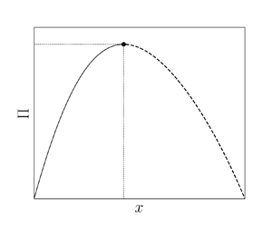
 Figure 1 displays the viscous potential from (2.32) as a function of Arina's dimensionless axis  $x/L$. By examining the graphics in that figure, one may observe that the sonic condition moves downstream up to
  $x/L=0.712$ where the viscous potential is a maximum
  $\varPi = 0.123$. Beyond that position, the sonic point cannot be attained any longer within the nozzle. Mathematical solutions to the right of the maximum displacement sonic point (dashed line) do not have physical meaning.

Figure 1. Viscous potential for a respective sonic point displacement, where the dashed line corresponds to the unphysical solution.
For a more general nozzle, where  $A(x)$ is known (2.33) displays a point of maximum for any geometry and viscous potential. That maximum condition is given the restriction that the
  $x$-derivative of (2.29) is null, which yields
 \begin{equation} \frac{{\rm d} (\varPi)}{{\rm d}\kern0.7pt x} =\frac{{\rm d}}{{\rm d}\kern0.7pt x}\left(\frac{1}{A} \frac{{\rm d} A}{{\rm d}\kern0.7pt x} \right)=0, \end{equation}
after carrying out the derivative, one obtains
 \begin{equation} A\frac{{\rm d}^{2} A}{{{\rm d}\kern0.7pt x}^{2}}-\left(\frac{{\rm d} A}{{\rm d}\kern0.7pt x} \right)^2=0. \end{equation}
Hence, the solution of (2.34) gives the maximum sonic point displacement position  $x_{max}$, which corresponds to the threshold of establishing a supersonic flow downstream of
  $x_{max}$. A higher
  $\varPi$ will inhibit a supersonic flow from being attained. Taking Arina's nozzle geometry as an example, consider a high-pressure and low-temperature supercritical oxygen state (
 $Gr=1.1$) and after employing (2.16) the maximum admissible
  $f/D_h$ value is
  $0.029$. In contrast, a low-pressure superheated oxygen exhibit a (
 $Gr=0.38$), resulting in a maximum admissible
  $f/D_h$ value of
  $0.044$. Therefore, the maximum normalised friction factor will depend on the fluid thermodynamic state.
2.3. Rankine–Hugoniot relations
If the nozzle exit pressure is higher than the environment discharging pressure, but lower than the critical subsonic solution, a normal shock wave should be formed within the nozzle. The Rankine–Hugoniot relations (2.35)–(2.37) are widely known for the treatment of discontinuities on compressible flows (e.g. shock waves, detonations (Thompson Reference Thompson1971b) or even evaporation waves (Simões-Moreira & Shepherd Reference Simões-Moreira and Shepherd1999) and condensation shocks (Bolaños-Acosta, Restrepo & Simões-Moreira Reference Bolaños-Acosta, Restrepo and Simões-Moreira2021)). The three conservation equations valid for a discontinuity are presented next, where the index 1 denotes the upstream state and 2 denotes the downstream state:
 \begin{gather} \rho_{1} V_{1} =\rho_{2} V_{2}, \end{gather}
 \begin{gather} \rho_{1} V_{1}^{2}+P_{1} =\rho_{2} V_{2}^{2}+P_{2}, \end{gather}
 \begin{gather} h_{1}+\frac{1}{2} V_{1}^{2} =h_{2}+\frac{1}{2} V_{2}^{2}. \end{gather}
2.4. Equation of state
The MPEOS used in this work was formulated in terms of the specific Helmholtz free energy, using experimental data fitted by optimisation algorithms Span (Reference Span2000). The classical definition of specific Helmholtz free energy is
 \begin{equation} a= e-Ts. \end{equation}
 The MPEOS is based on the non-dimensional Helmholtz free energy  $\alpha = a/ (RT)$, where
  $R$ is the universal gas constant. Here
  $\alpha$ can be calculated using the ideal
  $\alpha ^{0}$ and the residual part
  $\alpha ^{r}$. The residual part accounts for the real gas effects, and is calculated based on the polynomial, exponential and Gaussian bell-shaped terms corresponding to each substance,
 \begin{equation} \alpha=\alpha^{0}+\alpha^{r}. \end{equation}
Once the ideal and residual parts of the non-dimensional Helmholtz free energy are calculated, any thermodynamic property can be calculated as a derivative of the Helmholtz free energy, using the relations defined by
 \begin{equation} \left. \begin{aligned} \alpha_{\delta}^{{r}} & =\left(\frac{\partial \alpha^{{r}}}{\partial \delta}\right)_{\tau},\quad \alpha_{\delta \delta}^{{r}}=\left(\frac{\partial^{2} \alpha^{{r}}}{\partial \delta^{2}}\right)_{\tau}, \quad \alpha_{\delta \tau}^{{r}}=\left(\frac{\partial^{2} \alpha^{{r}}}{\partial \delta \partial \tau}\right),\\ \alpha_{\tau \tau}^{{o}} & =\left(\frac{\partial^{2} \alpha^{{\circ}}}{\partial \tau^{2}}\right)_{\delta}, \quad \alpha_{\tau \tau}^{{r}} =\left(\frac{\partial^{2} \alpha^{{r}}}{\partial \tau^{2}}\right)_{\delta}, \end{aligned} \right\} \end{equation}
where  $\tau = T_{c}/T$ is the non-dimensional temperature and
  $\delta = \rho /\rho _c$ is the non-dimensional density. The Grüneisen parameter can be computed from the following definition, where
  $\beta$ denotes the volume expansivity, which is derived from (2.11)
 \begin{equation} Gr = \frac{\beta c^2}{C_{P}}. \end{equation}
By substituting the definitions found in (2.40) into the non-dimensional Helmholtz free energy, one obtains
 \begin{equation} Gr ={-}\frac{\dfrac{1+\delta \alpha_{\delta}^{r}-\delta \tau \alpha_{\delta \tau}^{r}}{1+2 \delta \alpha_{\delta}^{r}+\delta^{2} \alpha_{\delta \delta}^{r}}\left(\dfrac{(1+\delta \alpha_{\delta}^{r}-\delta \tau \alpha_{\delta \tau}^{r})^{2}}{\tau^{2}\left(\alpha_{\tau \tau}^{{\circ}}+\alpha_{\tau \tau}^{r}\right)}-1-2 \delta \alpha_{\delta}^{r}-\delta^{2} \alpha_{\delta \delta}^{r}\right)}{\dfrac{\left(1+\delta \alpha_{\delta}^{r}-\delta \tau \alpha_{\delta \tau}^{r} \right)^{2}}{1+2 \delta \alpha_{\delta}^{r}+\delta^{2} \alpha_{\delta \delta}^{r}}-\tau^{2}\left(\alpha_{\tau \tau}^{{\circ}}+\alpha_{\tau \tau}^{r}\right)}. \end{equation}
 Figure 2 presents the  $Gr$ behaviour in a reduced temperature–specific entropy plane, for an oxygen MPEOS (Schmidt & Wagner Reference Schmidt and Wagner1985) and for an isobutane EOS (Bücker & Wagner Reference Bücker and Wagner2006) in superheated and supercritical phase, in addition, table 1 presents the thermodynamic properties (pressure, temperature and density) at the critical point for both evaluated fluids and the maximum operation pressure and temperature limits for each EOS. The figure shows the low variation of
  $Gr$ for superheated vapours. That trend applies to both fluids. However,
  $Gr$ steeply varies as the vapour phase becomes supercritical, especially for the region close to the critical point. A considerable difference can be perceived between both fluids due to their different molecular complexity, directly affecting the
  $Gr$ calculation, because, as the fluid molecule becomes more complex (e.g. BZT fluids), the
  $Gr$ value tends to decrease (Mausbach et al. Reference Mausbach, Köster, Rutkai, Thol and Vrabec2016), and this directly affects the viscous effects on the nozzle. The dynamic viscosity for both pure substances were computed after using the work of Lemmon & Jacobsen (Reference Lemmon and Jacobsen2004) and Vogel, Küchenmeister & Bich (Reference Vogel, Küchenmeister and Bich2000) for the oxygen and isobutane, respectively.

Figure 2. Grüneisen parameter variation for superheated and supercritical vapour of (a) oxygen and (b) isobutane.
Table 1. Critical properties and maximum pressure and temperature limits for oxygen and isobutane EOS.

2.5. Friction factor
The well-known Coolebrok–White equation was used to obtain the Darcy–Weisbach friction factor  $f_{D}$, where
  $\varepsilon$ denotes the channel surface roughness and
  ${Re}$ is the Reynolds number:
 \begin{equation} \frac{1}{\sqrt{f_{D}}}={-}2 \log \left(\frac{\varepsilon}{3.7 D_{{h}}}+\frac{2.51}{{Re} \sqrt{f_{D}}}\right). \end{equation}
 Note that the Darcy–Weisbach friction factor is four times the Fanning friction factor  $f=f_{D}/4$, and it is calculated for each computation step. The
  ${Re}$ number of rectangular cross-section channels were computed using the methodology proposed by Jones (Reference Jones1976) for different aspect ratio geometries.
3. Numerical solution
The numerical solution scheme of the real viscous gas compressible flow and the shock-wave position is depicted in figure 3; this control volume is discretised using constant steps  $\Delta x$. First, the sonic point location was found by the numerical root finding of (2.29) for the divergent nozzle part, where
  $Gr$ and
  $f$ values were initially computed for an isentropic sonic point located where
  $c(h_0,s_0)=V$. Next, the solution follows the HYBRD method (More, Garbow & Hillstrom Reference More, Garbow and Hillstrom1980) for the root finding and this routine was implemented through SciPy libraries (Virtanen et al. Reference Virtanen2020). After solving the sonic point, the algorithm uses the fourth-order Runge–Kutta method (RK-4) backwards until the nozzle inlet is reached. It was necessary to match the reservoir specific entropy
  $s_0$ to that from the solution obtained from the backwards RK-4 integration, because
  $s_{sonic}>s_0$ due to the entropy production (2.14), and this is performed through the
  $s_{sonic}$ variation using the HYBRD method. After computing the specific entropy at the sonic point, the algorithm proceeded forward using RK-4 until the nozzle exit was found.

Figure 3. Numerical solution procedure.
Note that for the sonic solution,  $M=1$, (2.15) cannot be solved as discussed in § 2.1, due to the indetermination of such an equation. Therefore, as the sonic point has been located, (2.28) was solved using a predictor–corrector finite difference scheme while
  $|M-1|<0.015$, for all the required derivatives and these equations were used to solve (2.28). This looping solution process continued until those derivatives matched the corresponding thermodynamic state after achieving a residual value from the last iteration less than
  ${1\times 10^{-8}}$.
Flow thermodynamic properties ( $c$,
$c$,  $C_P$,
  $k$,
$k$,  $Gr$) and dynamic viscosity were computed by using the code developed by Bell et al. (Reference Bell, Wronski, Quoilin and Lemort2014). In addition, a multidimensional solver was implemented using the HYBRD method for defining the thermodynamic state using specific enthalpy and specific entropy as independent variables
  $(h,s)$. Specific entropy and enthalpy were computed using (2.14) and (2.25), respectively, for each calculation step. If there was a shock wave inside the nozzle, a new stagnation condition was calculated considering the shock-wave downstream conditions obtained after solving the Rankine–Hugoniot relations (2.35)–(2.37) by using the HYBRD method. However, the shock-wave position depends on the exit pressure; this was thus computed using the Brent method for minimising the following function:
 \begin{equation} g(x)=|P_{Nozzle}-P_{e}|, \end{equation}
where  $P_{nozzle}$ is the final nozzle pressure with a shock-wave position inside the nozzle and
  $P_e$ is the exit pressure; therefore, the Brent minimisation method starts to march in space in the nozzle divergent part, seeking the condition whereby (3.1) is minimum after achieving a residual value from the last iteration less than
  ${1\times 10^{-8}}$. It is important to highlight that the proposed method is devoted to solving non-ideal classical flows
  $\varGamma >0$.
4. Results
4.1. Validation and verification
4.1.1. Perfect viscous gas flow verification
The first step in the proposed approach verification is to compare the developed methodology to the analytical viscous solution obtained by Ferrari (Reference Ferrari2021b). Ferrari's expression is developed for a viscid dilute gas in conical axisymmetric nozzles. Figure 4 presents the comparison outcomes for a different number of mesh nodes. Figure 4(a) is the subsonic solution obtained for the following conditions:  $L = 45$ cm, initial diameter
  $D_1 = 8$ cm, final diameter
  $D_2 = 3.5$ cm,
  $P_0 = 5$ bar,
  $T_0 = 500$ K,
  $M_1 = 0.11$ and
  $f = 0.004$. Figure 4(b) is the supersonic solution obtained for the following conditions:
  $L = 60$ cm, initial diameter
  $D_1 = 5$ cm, final diameter
  $D_2 = 9$ cm,
  $P_0 = 2$ bar,
  $T_0 = 400$ K,
  $M_1 = 1.1$ and
  $f = 0.006$. These results are obtained after using the Lemmon et al. (Reference Lemmon, Jacobsen, Penoncello and Friend2000) EOS. Figures 4(a) and 4(b) outcomes show the good performance of the developed method and display the mesh independence of the proposed numerical approach.

Figure 4. Ferrari (Reference Ferrari2021b) analytical and numerical results comparison: (a) subsonic and (b) supersonic solution.
4.1.2. Real viscous gas flow validation
Table 2 presents the experimental data from open literature used for validating the proposed methodology. That table presents in the first column the tested fluid, followed by stagnation properties ( $P_0$,
  $T_0$ and
  $Z_0$) used for each case with their respective references for the experimental data shown in the last column.
Table 2. Stagnation points and experimental data used for validation.

The experimental data reported by Spinelli et al. (Reference Spinelli, Cammi, Gallarini, Zocca, Cozzi, Gaetani, Dossena and Guardone2018) were used for the supersonic flow of octamethyltrisiloxane (MDM) (Thol et al. Reference Thol, Dubberke, Baumhögger, Vrabec and Span2017), for the dynamic viscosity computation it was used the approach proposed by Klein, McLinden & Laesecke (Reference Klein, McLinden and Laesecke1997). That substance has a high molecular weight ( $M=236.53\,\textrm {g}\,\textrm {mol}^{-1}$) and, due to this high molecular weight and complexity, this substance exhibits a non-ideal compressible behaviour near to the critical point. Considering the stagnation conditions presented in table 2, a numerical simulation was performed for a 750 uniformly spaced element mesh. Figure 5(a) presents the numerical simulation for the pressure profile. Figure 5(b) presents the Mach number comparison against the experimental results. Good agreement was found between the simulation and the experimental results. For the last pressure measurement, the deviation reached 7.2 %. In addition, the numerical simulation performed by Gori et al. (Reference Gori, Zocca, Cammi, Spinelli, Congedo and Guardone2020) was used to compare the MDM results with a multidimensional computational fluid dynamics (CFD) solver. After comparing the numerical outcome with the experimental data and the multidimensional solver, it was found that the proposed approach presents a good solution and the Mach number profile results represent the trend of the experimental outcomes.

Figure 5. Experimental results used for validation: (a) pressure profile and (b) Mach profile MDM; (c) pressure profile for water; (d) pressure profile for 75 % CO $_2$–air mixture; the black continuous line represents the numerical solution and the black solid points, the experimental data.
The EOS of Wagner & Pruß (Reference Wagner and Pruß2002) was used for the high-pressure steam simulation and the 4B nozzle of Gyarmathy (Reference Gyarmathy2005) was simulated using a 750-element mesh, which was found to be stable and mesh size independent. The approach of Huber et al. (Reference Huber, Perkins, Laesecke, Friend, Sengers, Assael, Metaxa, Vogel, Mareš and Miyagawa2009) was used for the dynamic viscosity estimation. High deviations in pressure (13.6 %) were found in this simulation for low supersonic Mach numbers; otherwise the simulation gave better results as the viscous effects became more relevant at the nozzle outlet where the pressure deviation fell (to 4.6 %).
For the mixture validation, the experimental data of Bier et al. (Reference Bier, Ehrler and Niekrawietz1990) were used for a mixture of carbon dioxide and atmospheric dry air. For the sake of simplicity air was treated as pure nitrogen using the GERG-2008 MPEOS (Kunz & Wagner Reference Kunz and Wagner2012). The formulation of Wilke (Reference Wilke1950) was used for the mixture dynamic viscosity calculation. Table 2 presents the stagnation conditions of the test, and figure 5(d) presents the pressure profile comparison between the experimental and simulation for a 500-element mesh.
Note that the dynamic viscosity computation has an important role in the solution. Nevertheless, not all fluids have dedicated models for their estimation, as in the MDM case. Therefore, the dynamic viscous model selection could be relevant on the model performance.
4.1.3. Shock-wave position verification
For the shock-wave model capturing verification, the same work by Arina (Reference Arina2004) was used due to its benchmark widespread use in supersonic nozzles flows. The MPEOS was used for air and nitrogen mixtures (Lemmon et al. Reference Lemmon, Jacobsen, Penoncello and Friend2000).
Figure 6 presents the nozzle pressure profile; the solution obtained by Arina (Reference Arina2004) was compared reproducing precisely the pressure jump and shock location.

Figure 6. Pressure distribution Arina's nozzle ( $P_0 = 100\,{\textrm {kPa}}$,
  $T_0 = 288 \,{\textrm {K}}$) for dry air.
4.2. Viscous effects on flow
The next set of analyses of the viscous effects on the Arina's nozzle is to compare the isentropic flow at the same stagnation conditions and nozzle geometry. Figure 7 presents the results for the supersonic expansion of two substances oxygen and isobutane for a stagnation pressure and temperature of ( $13.9\,{\textrm {MPa}}$,
  $240\,{\textrm {K}}$) and (
 $10\,{\textrm {MPa}}$,
  $520\,{\textrm {K}}$), respectively. Resulting in the same reduced pressure for both cases
  $P_r=P/P_c=2.75$. The stagnation temperature of the isobutane case was selected to display the fluid's non-ideal behaviour in the supersonic expansion; on the other hand, the oxygen case stagnation temperature was chosen to avoid the two-phase region achievement at the nozzle outlet.

Figure 7. Nozzle viscous effects, where simulations on the left correspond to isobutane and those on the right correspond to oxygen: (a,b) Pressure profile; (c,d) the Mach profile; (e,f) speed of sound profile on the nozzle; (g,h) Grüneisen parameter profile on the nozzle. Black continuous lines represent the isentropic expansion and dashed lines represent the viscous solution.
Both nozzles follow Arina geometrical design having the following geometric parameters:  $x_{th}=0.05\,{\textrm {m}}$,
  $L=0.1\,{\textrm {m}}$,
  $D_{th}={2\times 10^{-3}\,{\textrm {m}}}$,
  $\epsilon =1\times 10^{-6}\,{\textrm {m}}$ and a 1200- element mesh, obtained after ensuring a grid-independent result. Those parameters lead to small
  $\textrm {d}A/{\textrm {d}\kern0.06em x}$,
  $D_{h}$ and a high
  $f$, resulting in a high viscous effect. In the presented numerical examples, the viscous potential plays an important role in the supersonic expansion leading to a maximum point for the four evaluated variables (
 $P$,
$P$,  $M$,
$M$,  $c$,
$c$,  $Gr$) and for both fluids. This point results from the effects of the viscous potential on the velocity potential as seen in (2.15), and as
  $\varPi$ exceeds the area change rate, the velocity decreases and this leads to a change in all thermodynamics properties. For all figure 7 outcomes, the blue shaded region represents the viscid solution's departure from the isentropic solution.
4.2.1. Viscous effects on pressure profile
As presented before, the viscous effects are relevant and the nozzle behaviour departs from the isentropic flow as presented in figures 7(a) and 7(b) for the isobutane and oxygen pressure profile. The isobutane case achieved a slighter higher normalised friction factor  $f/D_h$ at the sonic point; nevertheless, the oxygen case deploys a higher
  $Gr$ value on the nozzle, resulting in an important change in the pressure profile. That occurs in part because of the change in the velocity potential as explained previously. In addition, the pressure profile shifts compared with the isentropic results due to the
  $\textrm {d}s/{\textrm {d}\kern0.06em x}$ increase, and this can be computed by substituting (2.14) into (2.10), resulting in
  $2Gr\rho V^2 f/D_h$. Therefore, the pressure profile shift is always positive and strongly influenced by the fluid velocity as seen in the deviation area in the pressure profiles in figures 7(a) and 7(b). Finally, if
  $Gr \rightarrow 0$, the pressure profile is closer to the isentropic profile as shown in figure 7(a) for isobutane, because isobutane has
  $Gr = 0.088$ at the sonic point compared with
  $Gr=0.47$ for oxygen.
4.2.2. Viscous effects on Mach number
Analogously, figures 7(c) and 7(d) present the viscous effects on the Mach profile and their corresponding maximum points. Even though oxygen has a higher  $Gr$, value at the sonic point compared with isobutane
  $Gr$; the sonic offset slightly changes for both fluids as can be seen in figures 7(c) and 7(d). In addition, the viscous effects lead to a decrease of the nozzle mass flow rate as a consequence of the sonic point shift.
4.2.3. Viscous effects on flow speed of sound
Finally, figures 7(e) and 7(f) present the speed of sound profile within the nozzle. The isobutane plot shows a non-monotonic behaviour, exhibiting the minimum and maximum points; the minimum point occurs due to the expansion of non-ideal gas behaviour represented by  $(\partial c/ \partial \rho )_s=0$. Therefore, the fluid expands into the non-ideal region, leading to an increase in the speed of sound until that the next maximum point is achieved due to the viscous effects. Thus, the speed of sound exhibits various inflexions points due to the combined effect of their non-ideal behaviour and the viscous effects as expected after inspecting (2.23). In addition, figures 7(e) and 7(f) show the difference in the speed of sound deviation between the isentropic and the viscid solution, because the offset for the oxygen case is considerably more evident than the isobutane due to the viscous effects on the last term of (2.23), so as
  $Gr \rightarrow 0$ the speed of sound profile will be closer to the isentropic solution.
4.2.4. Viscous effects on the Grüneisen parameter
As stressed out in the last sections the isobutane case presents lower  $Gr$ values than the oxygen case, and this originates a strong departure of the viscous solution after comparing both fluids. Even though the isobutane presents a non-ideal behaviour the Grüneisen parameter behaves in a similar fashion (figure 7g) to the oxygen case (figure 7h). However, the deviation of the viscous profile is more intense in the oxygen case than in the isobutane case.
4.2.5. Viscous effects on shock-wave intensity and position
Figure 8 presents the viscous effects on the intensity and shock-wave position for oxygen at the following stagnation conditions: ( $13.9\,{\textrm {MPa}}$,
  $240\,{\textrm {K}}$) employing an Arina nozzle with the following geometric parameters
  $x_{th}=0.05\,{\textrm {m}}$,
  $L=0.1\,{\textrm {m}}$,
  $D_{th}=4\times 10^{-3}\,{\textrm {m}}$ and three different values of surface roughness height (
 $\epsilon =1\times 10^{-7}\,{\textrm {m}}$,
  ${1\times 10^{-6}\,{\textrm {m}}}$,
  ${1\times 10^{-5}} \,{\textrm {m}}$) and an isentropic expansion for a 1200-element mesh. As presented in figure 8(a), all the simulations converge on the same exit pressure
  $0.72\times P_0$. Nevertheless, the pressure profile varies due to the viscous effects, because as long as the
  $f/D_h$ increases the shock-wave intensity decreases due to the Mach number reduction, leading to a small entropy increment by the shock wave. However, the viscous effects over the total specific entropy jump in the nozzle is stronger as the
  $f/D_h$ increases.

Figure 8. Viscous effects on the shock-wave formation for oxygen: (a) pressure profile, (b) Mach profile and (c) dimensionless specific entropy jump in the nozzle.
4.3. Nozzle performance
The analysis proposed allows important supersonic nozzle parameters to be calculated, i.e. discharge coefficient  $C_{d}$,
 \begin{equation} C_{d}=\frac{\dot{m}_{viscous}}{\dot{m}_{iso}}, \end{equation}
and nozzle efficiency  $\eta$,
 \begin{equation} \eta=\frac{h_0-h_e}{h_0-h_s}. \end{equation}
 The discharge coefficient captures the viscous effects over the ideal mass flow rate from a quasi-1D perspective, and the nozzle efficiency compares the actual kinetic energy at the nozzle exit against the kinetic energy corresponding to an isentropic expansion at the same exit pressure. Nevertheless, this works gives novel insights into the real gas effects on the nozzle performance. Figure 9 presents the effect of the stagnation condition on the  $C_{d}$ and
  $\eta$ values, for the following geometric variables for the Arina nozzle:
  $x_{th}=0.05\,{\textrm {m}}$,
  $L=0.1\,{\textrm {m}}$,
  $D_{th}={4\times 10^{-3}}\,{\textrm {m}}$ and
  $\epsilon ={1\times 10^{-6}}\,{\textrm {m}}$ for the 1200-uniformly-spaced-element mesh. Figures 9(a) and 9(b) show the
  $C_{d}$ and
  $\eta$ results for oxygen. These outcomes were obtained for several reduced stagnation pressures
  $P_0/P_c$ and temperatures
  $T_0/T_c$. Both variables have low values at low pressures due to the low
  ${Re}$ value and their subsequently high
  $f$ in such conditions and, as the pressure increases, the
  $C_{d}$ and
  $\eta$ reach their maximum value due to the
  ${Re}$ increase. However, if the pressure continues growing the nozzle performance decreases. This occurs due to the behaviour of the
  $Gr$ and its effect on the viscous effects; as can be seen in figure 2 the Grüneisen parameter increases in the supercritical region close to the critical point. In addition, after comparing figures 9(a)–9(c), it is possible to observe the inverse relationship between the nozzle performance and the viscous potential, because
  $\varPi$ shows the connection between the real and the viscous effects. Finally, figure 9(d) shows the compressibility factor outcome for the nozzles evaluated. Note that the simulations performed covered wide
  $Z$ values and the viscous potential is almost insensitive to such changes.

Figure 9. Nozzle performance for a supersonic oxygen nozzle: (a)  $C_{d}$, (b)
  $\eta$, (c) viscous potential at nozzle sonic point and (d) compressibility factor.
5. Conclusions
This work has presented a new real gas model for computing the viscous effects on convergent–divergent supersonic flows. The new formulation reveals the role of the Grüneisen parameter in the viscous flow; this model has been integrated with modern EOSs to achieve accurate results and even consider the non-ideal or supercritical effects on the flow. Moreover, this approach can be used for pure substances and for constant composition gas mixtures as long as they remain in the gas phase. This model has been validated against experimental data, leading to a good agreement for all the cases calculated.
Viscous effects on the sonic point formation have been studied showing that as the viscous potential increases, the sonic point moves towards to nozzle exit section. However, if the viscous potential achieves its maximum value, the nozzle does not reach the supersonic regime for any pressure ratio. Finally, it has been shown that for locally constant  $Gr$,
$Gr$,  $f$ values, the maximum viscous potential will be a function of the nozzle geometry.
Viscous effects may be strong enough to influence the velocity relation and invert their behaviour; this condition affects the flow thermodynamic properties (i.e. temperature, pressure and density). For non-ideal flows, viscous effects give additional inflexion points compared with an inviscid analysis. In addition, it was shown that the viscous potential affects the shock-wave position and strength.
The nozzle performance measured by its isentropic efficiency and discharge coefficient is highly dependent on the viscous potential, and due to the viscous and real gas effects, the nozzle performance achieves a maximum value for a certain stagnation condition and as the real gas effects (measured through the  $Gr$) increases or the
  ${Re}$ decreases the overall performance decreases.
Funding
We gratefully acknowledge support of the Research Centre for Gas Innovation (RCGI), hosted by the University of São Paulo (USP) and sponsored by the São Paulo Research Foundation (FAPESP 2014/50279-4) and Shell Brasil, and the strategic importance of the support given by ANP (Brazil's National Oil, Natural Gas and Biofuels Agency) through the R&D levy regulation.
Declaration of interests
The authors report no conflicts of interest.


