1 Introduction
If a body moves in a gas, then the frictional drag would be lower than that of the same body moving in a liquid because the frictional drag depends on the dynamic viscosity of a fluid. For example, the viscosity of water is approximately one hundred times larger than that of air. In addition, if there exists a fore–aft pressure difference which is proportional to the fluid density, the pressure drag or the form drag on a body in a gas also would be lower than that of the same body moving in a liquid. For example, the density of water is approximately one thousand times larger than that of air. Therefore, during its motion, if a body is completely enveloped in a single large gaseous cavity, the associated total drag is expected to be significantly reduced. This phenomenon is known as supercavitation. Thus, the creation and maintenance of supercavitation have been of great interest in naval applications such as a high-speed underwater vehicle, air lubrication of a ship hull, a high-speed torpedo etc. (Ceccio Reference Ceccio2010). The most relevant dimensionless number in the study of supercavitation is the cavitation number,
 $$\begin{eqnarray}\displaystyle \unicode[STIX]{x1D70E}_{c}=\frac{2(p_{r}-p_{c})}{\unicode[STIX]{x1D70C}V^{2}}, & & \displaystyle\end{eqnarray}$$
where
 $p_{r}$
is a reference or a background pressure,
$p_{r}$
is a reference or a background pressure,
 $p_{c}$
is the cavity pressure,
$p_{c}$
is the cavity pressure,
 $\unicode[STIX]{x1D70C}$
is the density of the surrounding liquid and
$\unicode[STIX]{x1D70C}$
is the density of the surrounding liquid and
 $V$
is the relative speed between the body and the surrounding liquid. In wetted flows (absent any cavity), the relevant dimensionless number is the pressure coefficient
$V$
is the relative speed between the body and the surrounding liquid. In wetted flows (absent any cavity), the relevant dimensionless number is the pressure coefficient
 $C_{p}=2(p_{x}-p_{r})/\unicode[STIX]{x1D70C}V^{2}$
, where
$C_{p}=2(p_{x}-p_{r})/\unicode[STIX]{x1D70C}V^{2}$
, where
 $p_{x}$
is the local pressure at a specific location. Therefore, in cavity flows,
$p_{x}$
is the local pressure at a specific location. Therefore, in cavity flows,
 $\unicode[STIX]{x1D70E}_{c}=-C_{p}$
. A relatively small cavitation number is more favourable for supercavitation; a relatively high-speed natural supercavitation and a relatively low-speed ventilated supercavitation. Many similarities exist between a natural supercavitation and a ventilated supercavitation. For example, the sizes of both types of cavities scale with the cavitation number in approximately the same way. Outside of the time-averaged cavity shapes, however, the physics are quite different. This is especially true when one begins to look at the cavity dynamics. Given the fact that the fundamental physics regarding the time-averaged cavity shapes are the same for both types of supercavitation, many previous experimental studies have been done on ventilated supercavitation instead of a natural one which is more difficult to achieve or to definitively observe in laboratory environments (Logvinovich Reference Logvinovich1972; Epshtein Reference Epshtein1973; Hrubes Reference Hrubes2001; Spurk & König Reference Spurk and König2002; Schaffar et al.
Reference Schaffar, Rey and Boeglen2005; Cameron et al.
Reference Cameron, Rogers, Doane and Gifford2011). Furthermore, many prior studies on ventilated supercavitation have been done exclusively in closed water-circulation tunnels rather than open environments (Self & Ripken Reference Self and Ripken1955; Cox & Clayden Reference Cox and Clayden1956; Schauer Reference Schauer2003; Kawakami Reference Kawakami2010; Zhou et al.
Reference Zhou, Yu, Min and Yang2010; Haipeng et al.
Reference Haipeng, Song, Qin, Biao and Guoyu2014; Nouri et al.
Reference Nouri, Madoliat, Jahangardy and Abdolahi2015; Karn et al.
Reference Karn, Arndt and Hong2016). In these kinds of closed water-tunnel studies, various steady-state supercavity formations or cavity-closure modes have been observed based on some representative dimensionless numbers; the cavitation number
$\unicode[STIX]{x1D70E}_{c}=-C_{p}$
. A relatively small cavitation number is more favourable for supercavitation; a relatively high-speed natural supercavitation and a relatively low-speed ventilated supercavitation. Many similarities exist between a natural supercavitation and a ventilated supercavitation. For example, the sizes of both types of cavities scale with the cavitation number in approximately the same way. Outside of the time-averaged cavity shapes, however, the physics are quite different. This is especially true when one begins to look at the cavity dynamics. Given the fact that the fundamental physics regarding the time-averaged cavity shapes are the same for both types of supercavitation, many previous experimental studies have been done on ventilated supercavitation instead of a natural one which is more difficult to achieve or to definitively observe in laboratory environments (Logvinovich Reference Logvinovich1972; Epshtein Reference Epshtein1973; Hrubes Reference Hrubes2001; Spurk & König Reference Spurk and König2002; Schaffar et al.
Reference Schaffar, Rey and Boeglen2005; Cameron et al.
Reference Cameron, Rogers, Doane and Gifford2011). Furthermore, many prior studies on ventilated supercavitation have been done exclusively in closed water-circulation tunnels rather than open environments (Self & Ripken Reference Self and Ripken1955; Cox & Clayden Reference Cox and Clayden1956; Schauer Reference Schauer2003; Kawakami Reference Kawakami2010; Zhou et al.
Reference Zhou, Yu, Min and Yang2010; Haipeng et al.
Reference Haipeng, Song, Qin, Biao and Guoyu2014; Nouri et al.
Reference Nouri, Madoliat, Jahangardy and Abdolahi2015; Karn et al.
Reference Karn, Arndt and Hong2016). In these kinds of closed water-tunnel studies, various steady-state supercavity formations or cavity-closure modes have been observed based on some representative dimensionless numbers; the cavitation number
 $\unicode[STIX]{x1D70E}_{c}$
in (1.1), and the Froude number
$\unicode[STIX]{x1D70E}_{c}$
in (1.1), and the Froude number
 $$\begin{eqnarray}\displaystyle Fr=\frac{V}{\sqrt{gd_{c}}}, & & \displaystyle\end{eqnarray}$$
the air-entrainment coefficient
 $$\begin{eqnarray}\displaystyle C_{q}=\frac{Q}{d_{c}^{2}V}, & & \displaystyle\end{eqnarray}$$
and the blockage ratio
 $$\begin{eqnarray}\displaystyle B=\frac{d_{c}}{d_{h}};\quad d_{h}=\frac{4A_{c}(\text{cross-sectional area})}{P(\text{wetted perimeter})}. & & \displaystyle\end{eqnarray}$$
Here,
 $g$
is the gravitational acceleration,
$g$
is the gravitational acceleration,
 $d_{c}$
is the diameter of the disk-type cavitator,
$d_{c}$
is the diameter of the disk-type cavitator,
 $Q$
is the ventilated gas volumetric flow rate and
$Q$
is the ventilated gas volumetric flow rate and
 $d_{h}$
is the hydraulic diameter of a tunnel. Well-known examples of steady-state cavity formations are the foamy cavity, twin-vortex supercavity (Cox & Clayden Reference Cox and Clayden1956; Kawakami Reference Kawakami2010; Zhou et al.
Reference Zhou, Yu, Min and Yang2010), quad-vortex supercavity (Kapankin & Gusev Reference Kapankin and Gusev1984; Kawakami & Arndt Reference Kawakami and Arndt2011), reentrant-jet supercavity (Gadd & Grant Reference Gadd and Grant1965; Skidmore Reference Skidmore2013) and pulsating supercavity (Silberman & Song Reference Silberman and Song1961; Song Reference Song1961; Karlikov et al.
Reference Karlikov, Reznichenko, Khomyakov and Sholomovich1987; Semenenko Reference Semenenko2001a
; Semenenko Reference Semenenko2001b
; Skidmore Reference Skidmore2013). These different supercavity formations are quantitatively differentiated according to certain relationships between some of dimensionless parameters
$d_{h}$
is the hydraulic diameter of a tunnel. Well-known examples of steady-state cavity formations are the foamy cavity, twin-vortex supercavity (Cox & Clayden Reference Cox and Clayden1956; Kawakami Reference Kawakami2010; Zhou et al.
Reference Zhou, Yu, Min and Yang2010), quad-vortex supercavity (Kapankin & Gusev Reference Kapankin and Gusev1984; Kawakami & Arndt Reference Kawakami and Arndt2011), reentrant-jet supercavity (Gadd & Grant Reference Gadd and Grant1965; Skidmore Reference Skidmore2013) and pulsating supercavity (Silberman & Song Reference Silberman and Song1961; Song Reference Song1961; Karlikov et al.
Reference Karlikov, Reznichenko, Khomyakov and Sholomovich1987; Semenenko Reference Semenenko2001a
; Semenenko Reference Semenenko2001b
; Skidmore Reference Skidmore2013). These different supercavity formations are quantitatively differentiated according to certain relationships between some of dimensionless parameters
 $Fr$
,
$Fr$
,
 $\unicode[STIX]{x1D70E}_{c}$
,
$\unicode[STIX]{x1D70E}_{c}$
,
 $C_{q}$
and
$C_{q}$
and
 $B$
, depending on separate studies. An axisymmetric reentrant-jet supercavity occurs when the
$B$
, depending on separate studies. An axisymmetric reentrant-jet supercavity occurs when the
 $Fr$
is high or when the gravitational force is negligible compared to the inertia force. The twin-vortex supercavity occurs when the
$Fr$
is high or when the gravitational force is negligible compared to the inertia force. The twin-vortex supercavity occurs when the
 $Fr$
is low or when the gravity effect is not negligible any more. In these kinds of closed or bounded environments, the blockage effect always exists, which favours the occurrence of the twin-vortex supercavity rather than the reentrant-jet supercavity (Karn et al.
Reference Karn, Arndt and Hong2016). Karn et al. (Reference Karn, Arndt and Hong2016) posit that the closure mechanism is mainly determined by the pressure difference across the gas–water interface at the cavity closure. For the reentrant-jet (RJ) supercavity, the pressure difference is dominated by the momentum of the reentrant water jet, while for a twin-vortex (TV) supercavity, such a difference is much smaller. Based on the liner momentum theorem, they suggest a formula showing that the pressure difference monotonically decreases as the blockage ratio increases or vice versa. Therefore, in a closed environment, a higher blockage (
$Fr$
is low or when the gravity effect is not negligible any more. In these kinds of closed or bounded environments, the blockage effect always exists, which favours the occurrence of the twin-vortex supercavity rather than the reentrant-jet supercavity (Karn et al.
Reference Karn, Arndt and Hong2016). Karn et al. (Reference Karn, Arndt and Hong2016) posit that the closure mechanism is mainly determined by the pressure difference across the gas–water interface at the cavity closure. For the reentrant-jet (RJ) supercavity, the pressure difference is dominated by the momentum of the reentrant water jet, while for a twin-vortex (TV) supercavity, such a difference is much smaller. Based on the liner momentum theorem, they suggest a formula showing that the pressure difference monotonically decreases as the blockage ratio increases or vice versa. Therefore, in a closed environment, a higher blockage (
 $B$
) leads to a smaller pressure difference, promoting the occurrence of a twin-vortex supercavity. Comparatively, in unbounded environments, the blockage effect from a wall does not exist. Therefore, with no dependence on the blockage ratio, the open-environment supercavity formation will depend only on the Froude number, the cavitation number and the air entrainment coefficient. In a free-surface environment, the blockage effect may be small but finite; thus, the associated blockage ratio can be similarly defined to that of a closed environment. Therefore, in this case, the various types of supercavity formations will depend on the cavitation number (1.1), the Froude number (1.2), the air-entrainment coefficient (1.3) and the blockage ratio (1.4). Moreover, various types of supercavity formations may depend on the closeness of a body to the free surface and the existence of a body, which are dimensionlessly represented, respectively, by
$B$
) leads to a smaller pressure difference, promoting the occurrence of a twin-vortex supercavity. Comparatively, in unbounded environments, the blockage effect from a wall does not exist. Therefore, with no dependence on the blockage ratio, the open-environment supercavity formation will depend only on the Froude number, the cavitation number and the air entrainment coefficient. In a free-surface environment, the blockage effect may be small but finite; thus, the associated blockage ratio can be similarly defined to that of a closed environment. Therefore, in this case, the various types of supercavity formations will depend on the cavitation number (1.1), the Froude number (1.2), the air-entrainment coefficient (1.3) and the blockage ratio (1.4). Moreover, various types of supercavity formations may depend on the closeness of a body to the free surface and the existence of a body, which are dimensionlessly represented, respectively, by
 $$\begin{eqnarray}\displaystyle & \displaystyle h^{\ast }=\frac{h_{s}}{H}, & \displaystyle\end{eqnarray}$$
 $$\begin{eqnarray}\displaystyle & \displaystyle d^{\ast }=\frac{d_{c}}{d}=\left\{\begin{array}{@{}l@{}}\text{finite (body)}\\ \infty ~(\text{no body}),\end{array}\right. & \displaystyle\end{eqnarray}$$
where
 $h_{s}$
is the submergence depth of a body,
$h_{s}$
is the submergence depth of a body,
 $H$
is the water depth,
$H$
is the water depth,
 $d$
is the diameter of the body and
$d$
is the diameter of the body and
 $d_{c}$
is the diameter of the cavitator. For example, six parameters (1.1)–(1.6) will determine the shape of a reentrant-jet (RJ) type supercavity which can be approximated as an ellipsoid with a length (
$d_{c}$
is the diameter of the cavitator. For example, six parameters (1.1)–(1.6) will determine the shape of a reentrant-jet (RJ) type supercavity which can be approximated as an ellipsoid with a length (
 $l$
), a width (
$l$
), a width (
 $w$
) and a height (
$w$
) and a height (
 $h$
) or dimensionlessly with reference to a cavitator diameter
$h$
) or dimensionlessly with reference to a cavitator diameter
 $d_{c}$
,
$d_{c}$
,
 $$\begin{eqnarray}\displaystyle & \displaystyle l^{\ast }=\frac{l}{d_{c}}, & \displaystyle\end{eqnarray}$$
 $$\begin{eqnarray}\displaystyle & \displaystyle w^{\ast }=\frac{w}{d_{c}}, & \displaystyle\end{eqnarray}$$
 $$\begin{eqnarray}\displaystyle & \displaystyle h^{\ast }=\frac{h}{d_{c}}. & \displaystyle\end{eqnarray}$$
In addition, for each type of supercavity formation, the drag coefficient (
 $C_{d}$
) based on the frontal area of a moving body can be measured and compared to a non-supercavitating moving body according to the body-diameter-based Reynolds number (
$C_{d}$
) based on the frontal area of a moving body can be measured and compared to a non-supercavitating moving body according to the body-diameter-based Reynolds number (
 $Re_{d}$
).
$Re_{d}$
).
 $$\begin{eqnarray}\displaystyle & \displaystyle C_{d}=\frac{F_{D}}{\displaystyle \frac{1}{2}\unicode[STIX]{x1D70C}V^{2}\left(\frac{\unicode[STIX]{x03C0}}{4}d^{2}\right)} & \displaystyle\end{eqnarray}$$
 $$\begin{eqnarray}\displaystyle & \displaystyle Re_{d}=\frac{\unicode[STIX]{x1D70C}Vd}{\unicode[STIX]{x1D707}}, & \displaystyle\end{eqnarray}$$
where,
 $F_{D}$
is the drag force,
$F_{D}$
is the drag force,
 $\unicode[STIX]{x1D70C}$
is the density of a liquid and
$\unicode[STIX]{x1D70C}$
is the density of a liquid and
 $\unicode[STIX]{x1D707}$
is the dynamic viscosity of a liquid. To the best of the present authors’ knowledge, all these themes have not been well addressed in previous experimental studies in free-surface environments, although there have been a few relevant experimental studies (Campbell & Hilborne Reference Campbell and Hilborne1958; Kuklinski et al.
Reference Kuklinski, Henoch and Castano2001). Campbell & Hilborne (Reference Campbell and Hilborne1958) conducted experiments on the formation of steady-state RJ and TV supercavities in a circular free-surface water channel (water depth: 0.46 m, channel width: 0.91 m, submergence depth: 0.22 m) with disk-type cavitators (diameter: 0.013 m, 0.019 m, 0.025 m, corresponding blockage ratio
$\unicode[STIX]{x1D707}$
is the dynamic viscosity of a liquid. To the best of the present authors’ knowledge, all these themes have not been well addressed in previous experimental studies in free-surface environments, although there have been a few relevant experimental studies (Campbell & Hilborne Reference Campbell and Hilborne1958; Kuklinski et al.
Reference Kuklinski, Henoch and Castano2001). Campbell & Hilborne (Reference Campbell and Hilborne1958) conducted experiments on the formation of steady-state RJ and TV supercavities in a circular free-surface water channel (water depth: 0.46 m, channel width: 0.91 m, submergence depth: 0.22 m) with disk-type cavitators (diameter: 0.013 m, 0.019 m, 0.025 m, corresponding blockage ratio
 $B=1.4\,\%$
, 2.1 %, 2.8 % for
$B=1.4\,\%$
, 2.1 %, 2.8 % for
 $h^{\ast }=0.47$
). Kuklinski et al. (Reference Kuklinski, Henoch and Castano2001) did experiments on the dynamics of ventilated supercavitation in a straight free-surface channel (water depth: 3.6 m, channel width: 7.3 m, no information about the submergence depth) with a disk-type cavitator (
$h^{\ast }=0.47$
). Kuklinski et al. (Reference Kuklinski, Henoch and Castano2001) did experiments on the dynamics of ventilated supercavitation in a straight free-surface channel (water depth: 3.6 m, channel width: 7.3 m, no information about the submergence depth) with a disk-type cavitator (
 $B=2\,\%$
) and cone-type cavitators. The theme of Campbell & Hilborne’s (Reference Campbell and Hilborne1958) work is closer to that of the present experimental study. They showed that an RJ supercavity occurs when
$B=2\,\%$
) and cone-type cavitators. The theme of Campbell & Hilborne’s (Reference Campbell and Hilborne1958) work is closer to that of the present experimental study. They showed that an RJ supercavity occurs when
 $\unicode[STIX]{x1D70E}_{c}Fr>1$
, and a TV supercavity occurs when
$\unicode[STIX]{x1D70E}_{c}Fr>1$
, and a TV supercavity occurs when
 $\unicode[STIX]{x1D70E}_{c}Fr<1$
(which will be shown not to agree with the present study). For the case of
$\unicode[STIX]{x1D70E}_{c}Fr<1$
(which will be shown not to agree with the present study). For the case of
 $B=3\,\%$
for
$B=3\,\%$
for
 $h^{\ast }=0.5$
in the present study, we observe diverse supercavities, which were not observed in their work for a similar condition
$h^{\ast }=0.5$
in the present study, we observe diverse supercavities, which were not observed in their work for a similar condition
 $B=2.8\,\%$
and
$B=2.8\,\%$
and
 $h^{\ast }=0.47$
. In addition, they did not consider the effect of the closeness of the free surface on the formation of supercavities. Therefore, these are the subjects of the present paper. From the towing tank experiment with a free-surface environment, we observe different types of supercavity formations at steady state depending on the cavitation number (1.1), the Froude number (1.2), the air-entrainment coefficient (1.3), the blockage ratio (1.4), the closeness of a body to the free surface (1.5) and the existence of a body (1.6). In particular, for a reentrant-jet type supercavity, we measure the ellipsoidal shape in terms of the dimensionless length, width and height (1.7)–(1.9) in the following form.
$h^{\ast }=0.47$
. In addition, they did not consider the effect of the closeness of the free surface on the formation of supercavities. Therefore, these are the subjects of the present paper. From the towing tank experiment with a free-surface environment, we observe different types of supercavity formations at steady state depending on the cavitation number (1.1), the Froude number (1.2), the air-entrainment coefficient (1.3), the blockage ratio (1.4), the closeness of a body to the free surface (1.5) and the existence of a body (1.6). In particular, for a reentrant-jet type supercavity, we measure the ellipsoidal shape in terms of the dimensionless length, width and height (1.7)–(1.9) in the following form.
 $$\begin{eqnarray}\displaystyle \frac{l}{d_{c}},\frac{w}{d_{c}},\frac{h}{d_{c}}=fcn\left(Fr,C_{q},\unicode[STIX]{x1D70E}_{c},B,\frac{d_{c}}{d},\frac{h_{s}}{H},Re_{d}\right). & & \displaystyle\end{eqnarray}$$
In addition, for each type of supercavity formation, we measure the drag coefficient (1.10) based on the frontal area of a moving body,
 $$\begin{eqnarray}\displaystyle C_{d}=fcn\left(Fr,C_{q},\unicode[STIX]{x1D70E}_{c},B,\frac{d_{c}}{d},\frac{h_{s}}{H},Re_{d}\right) & & \displaystyle\end{eqnarray}$$
and, therefore, estimate the amount of drag reduction compared to a non-supercavitating moving body according to the body-diameter-based Reynolds number (
 $Re_{d}$
). As a simple check of (1.12) and (1.13) in view of dimensional analysis, because we have fourteen dimensional parameters (
$Re_{d}$
). As a simple check of (1.12) and (1.13) in view of dimensional analysis, because we have fourteen dimensional parameters (
 $\unicode[STIX]{x1D70C}$
,
$\unicode[STIX]{x1D70C}$
,
 $\unicode[STIX]{x1D707}$
,
$\unicode[STIX]{x1D707}$
,
 $h_{s}$
,
$h_{s}$
,
 $d_{c}$
,
$d_{c}$
,
 $V$
,
$V$
,
 $Q$
,
$Q$
,
 $p_{c}$
,
$p_{c}$
,
 $d$
,
$d$
,
 $g$
,
$g$
,
 $H(d_{h})$
,
$H(d_{h})$
,
 $l$
,
$l$
,
 $w$
,
$w$
,
 $h$
,
$h$
,
 $F_{d}$
), there will be
$F_{d}$
), there will be
 $14-3=11$
dimensionless parameters, where the number of independent dimensional parameters is three in terms of their dimensions.
$14-3=11$
dimensionless parameters, where the number of independent dimensional parameters is three in terms of their dimensions.
In the next section § 2, the detailed experimental set-up and procedures are explained. In the experiment, depending on the ratio of the size of the cavitator to that of the body (1.6), the blockage ratio (1.4) and the closeness of a body to the free surface (1.5), four different cases are considered both when a body exists (
 $d\neq 0$
in (1.6)) behind a cavitator and three different cases when a body does not exist (
$d\neq 0$
in (1.6)) behind a cavitator and three different cases when a body does not exist (
 $d=0$
in (1.6)) behind a cavitator. As will be shown, both cases result in almost the same results in terms of steady-state phenomena including supercavity formation. In other words, the dimensionless parameter
$d=0$
in (1.6)) behind a cavitator. As will be shown, both cases result in almost the same results in terms of steady-state phenomena including supercavity formation. In other words, the dimensionless parameter
 $d^{\ast }=d_{c}/d$
(1.6) is excluded from the parameter space. In § 3, for each case, observation of various steady-state phenomena, including supercavity formation, are presented depending on the variation of the relevant dimensionless parameters. In the present work, the role of viscosity (
$d^{\ast }=d_{c}/d$
(1.6) is excluded from the parameter space. In § 3, for each case, observation of various steady-state phenomena, including supercavity formation, are presented depending on the variation of the relevant dimensionless parameters. In the present work, the role of viscosity (
 $\unicode[STIX]{x1D707}$
) or the Reynolds number (
$\unicode[STIX]{x1D707}$
) or the Reynolds number (
 $Re_{d}$
) is not included in supercavity formation. Dimensional parameters are the volumetric flow rate, the body speed and the resultant pressure behind the moving body (cavity pressure in the case of supercavity formation). The former two are the independent variables before each test and the latter is the dependent variable after each test. The equivalent dimensionless parameters are the Froude number, the air-entrainment coefficient and the cavitation number (for the existence of a cavity) or the pressure coefficient (in the absence of a cavity) where the relevant length scale is the diameter of the cavitator or the body depending on the existence of a cavitator. Then, for example, for a reentrant-jet type supercavity, their dimensionless lengths, widths, and heights are measured according to the following dimensionless parameters, neglecting the effects of
$Re_{d}$
) is not included in supercavity formation. Dimensional parameters are the volumetric flow rate, the body speed and the resultant pressure behind the moving body (cavity pressure in the case of supercavity formation). The former two are the independent variables before each test and the latter is the dependent variable after each test. The equivalent dimensionless parameters are the Froude number, the air-entrainment coefficient and the cavitation number (for the existence of a cavity) or the pressure coefficient (in the absence of a cavity) where the relevant length scale is the diameter of the cavitator or the body depending on the existence of a cavitator. Then, for example, for a reentrant-jet type supercavity, their dimensionless lengths, widths, and heights are measured according to the following dimensionless parameters, neglecting the effects of
 $d_{c}/d$
and
$d_{c}/d$
and
 $Re_{d}$
.
$Re_{d}$
.
 $$\begin{eqnarray}\displaystyle \frac{l}{d_{c}},\frac{w}{d_{c}},\frac{h}{d_{c}}=fcn\left(Fr,C_{q},\unicode[STIX]{x1D70E}_{c},B,\frac{h_{s}}{H}\right), & & \displaystyle\end{eqnarray}$$
which are compared with existing theoretical and semi-empirical results. Finally, in § 4, the associated drags of the various steady states in § 3 are measured and compared with each other according to the Reynolds numbers based on the body diameter, from which the effect of supercavitation on the drag reduction can be clearly seen. The drag coefficient can be expressed as follows, neglecting the effect of
 $d_{c}/d$
.
$d_{c}/d$
.
 $$\begin{eqnarray}\displaystyle C_{d}=fcn\left(Fr,C_{q},\unicode[STIX]{x1D70E}_{c},B,\frac{h_{s}}{H},Re_{d}\right). & & \displaystyle\end{eqnarray}$$
2 Experimental set-up

Figure 1. Schematics of the experimental set-up ((a) side view, (b) front view).
To make observations of the supercavitation phenomenon around a moving underwater body in a still fluid, a specialized towing water tank was designed and installed, as shown in schematics of figure 1. The tank size is 19.2 m long, 1 m wide and 1 m high and the side walls of the tank are made of transparent glass for visual observation from the outside. The towing system is a combination of a remodelled battery-driven remote control (RC) car and two straight rails which are laid on the two sides atop and along the entire length of the water tank. The RC car can run with a maximum speed of
 $7~\text{m}~\text{s}^{-1}$
along the rails, and the RC car and the underwater body are rigidly attached to each other through a right-angled C-shaped connecting rod, and, thus, the underwater body is driven by the RC car with the same speed. The use of the right-angled C-shaped rod (diameter: 10 mm) is to minimize the influence of the rod on the flow and the cavity formation around the moving underwater body. In the test, the speed range is
$7~\text{m}~\text{s}^{-1}$
along the rails, and the RC car and the underwater body are rigidly attached to each other through a right-angled C-shaped connecting rod, and, thus, the underwater body is driven by the RC car with the same speed. The use of the right-angled C-shaped rod (diameter: 10 mm) is to minimize the influence of the rod on the flow and the cavity formation around the moving underwater body. In the test, the speed range is
 $1{-}7~\text{m}~\text{s}^{-1}$
, therefore the relevant Reynolds number based on the rod diameter is between 10 000 and 70 000. In this flow regime, there is a laminar boundary layer separation at
$1{-}7~\text{m}~\text{s}^{-1}$
, therefore the relevant Reynolds number based on the rod diameter is between 10 000 and 70 000. In this flow regime, there is a laminar boundary layer separation at
 $80^{\circ }$
and the associated wake is completely turbulent with a vortex shedding (Panton Reference Panton2005; Sumer & Fredsoe Reference Sumer and Fredsoe2010). Regardless of this vortex shedding, we checked that the whole C-shaped rod/stinger mount system is sufficiently rigid to prevent the vibration of a body to which a cavitator is attached. We checked our image data using pixels for the rigidity of the body. Most of the time at the steady state during a running test, the variation of the movement is very difficult to identify even from the pixel test. There are some rare intermittent moments only during the acceleration and the deceleration, however, in which the body moves less than 1 pixel. Since our 1 pixel corresponds to 4.7 mm, the movement is less than 4.7 mm. Therefore, considering the body length (90 mm), the relative movement is less than
$80^{\circ }$
and the associated wake is completely turbulent with a vortex shedding (Panton Reference Panton2005; Sumer & Fredsoe Reference Sumer and Fredsoe2010). Regardless of this vortex shedding, we checked that the whole C-shaped rod/stinger mount system is sufficiently rigid to prevent the vibration of a body to which a cavitator is attached. We checked our image data using pixels for the rigidity of the body. Most of the time at the steady state during a running test, the variation of the movement is very difficult to identify even from the pixel test. There are some rare intermittent moments only during the acceleration and the deceleration, however, in which the body moves less than 1 pixel. Since our 1 pixel corresponds to 4.7 mm, the movement is less than 4.7 mm. Therefore, considering the body length (90 mm), the relative movement is less than
 $4.7/90=5.2\,\%$
at worst, only during the acceleration and deceleration. The speed of the RC car or the underwater body is digitally controlled and varied from
$4.7/90=5.2\,\%$
at worst, only during the acceleration and deceleration. The speed of the RC car or the underwater body is digitally controlled and varied from
 $1$
to
$1$
to
 $7~\text{m}~\text{s}^{-1}$
at steady state in the experiment (figure 2). The time interval of a steady state depends on the speed of the RC car due to the finite length of the tank; with each target constant speed in mind, first, the position of the underwater body is identified according to time from the video-recording data (figure 2
a). For all cases, the driving distance is 17.5 m. Then, the instantaneous speed of the moving body is obtained by calculating the slope of two consecutive position data during a corresponding time interval (figure 2
b). In figure 2(b), one can see three phases; the accelerating phase, the constant-speed phase and the decelerating phase. Low-speed cases have relatively longer accelerating and constant-speed phases compared to the high-speed cases. In particular, for constant-speed observations, we have time of approximately 15 s for the case of
$7~\text{m}~\text{s}^{-1}$
at steady state in the experiment (figure 2). The time interval of a steady state depends on the speed of the RC car due to the finite length of the tank; with each target constant speed in mind, first, the position of the underwater body is identified according to time from the video-recording data (figure 2
a). For all cases, the driving distance is 17.5 m. Then, the instantaneous speed of the moving body is obtained by calculating the slope of two consecutive position data during a corresponding time interval (figure 2
b). In figure 2(b), one can see three phases; the accelerating phase, the constant-speed phase and the decelerating phase. Low-speed cases have relatively longer accelerating and constant-speed phases compared to the high-speed cases. In particular, for constant-speed observations, we have time of approximately 15 s for the case of
 $1~\text{m}~\text{s}^{-1}$
and approximately 1 s for the case of
$1~\text{m}~\text{s}^{-1}$
and approximately 1 s for the case of
 $7~\text{m}~\text{s}^{-1}$
. We set-up seven speeds 1, 2, 3, 4, 5, 6,
$7~\text{m}~\text{s}^{-1}$
. We set-up seven speeds 1, 2, 3, 4, 5, 6,
 $7~\text{m}~\text{s}^{-1}$
due to the limitation of the tank length. We checked that the digitally controlled speed of the RC car show almost zero input–output discrepancy and almost zero variation from the target speed at steady state. For the real-time observation of supercavity formation around the moving underwater body, two video-recording cameras (Sony HDR-AS100V, 240 fps,
$7~\text{m}~\text{s}^{-1}$
due to the limitation of the tank length. We checked that the digitally controlled speed of the RC car show almost zero input–output discrepancy and almost zero variation from the target speed at steady state. For the real-time observation of supercavity formation around the moving underwater body, two video-recording cameras (Sony HDR-AS100V, 240 fps,
 $800\times 480$
pixels) are attached to the towing system as shown in figure 1. The camera near the tank wall is for the side view observation of supercavitation and that at the bottom of the RC car is for the top view observation of supercavitation. For the video recording of the clear side view observation, black papers are glued to the opposite side of the tank wall to minimize the reflection of light. For the present ventilated supercavitation experiment, as mentioned in the introduction, the important dimensionless number is the cavitation number or the relative underpressure of the cavity,
$800\times 480$
pixels) are attached to the towing system as shown in figure 1. The camera near the tank wall is for the side view observation of supercavitation and that at the bottom of the RC car is for the top view observation of supercavitation. For the video recording of the clear side view observation, black papers are glued to the opposite side of the tank wall to minimize the reflection of light. For the present ventilated supercavitation experiment, as mentioned in the introduction, the important dimensionless number is the cavitation number or the relative underpressure of the cavity,

Figure 2. Position and speed of the underwater body versus time. (a) Position versus time, (b) speed versus time.

Figure 3. Torpedo-shaped (cylinder capped with hemispherical ends) underwater bodies (weight: 140 g) (a) without a cavitator, (b) with a small disk-type cavitator (diameter: 15 mm, weight: 15 g), (c) with a large disk-type cavitator (diameter: 30 mm, weight: 22 g).
 $$\begin{eqnarray}\displaystyle \unicode[STIX]{x1D70E}_{c}=\frac{2(p_{r}-p_{c})}{\unicode[STIX]{x1D70C}V^{2}}=\frac{2(p_{atm}+\unicode[STIX]{x1D70C}gh_{s}-p_{c})}{\unicode[STIX]{x1D70C}V^{2}}, & & \displaystyle\end{eqnarray}$$
where
 $h_{s}$
is the submergence depth of the centre of the moving body from the free surface. The cavity pressure
$h_{s}$
is the submergence depth of the centre of the moving body from the free surface. The cavity pressure
 $p_{c}$
is measured using a film-type pressure sensor (Teksan FlexiForce A201, Operation range: 39 000–163 700 Pa at
$p_{c}$
is measured using a film-type pressure sensor (Teksan FlexiForce A201, Operation range: 39 000–163 700 Pa at
 $-40{-}60\,^{\circ }\text{C}$
, nonlinearity error
$-40{-}60\,^{\circ }\text{C}$
, nonlinearity error
 ${<}$
${<}$
 $\pm$
3 % F.S., repeatability error
$\pm$
3 % F.S., repeatability error
 ${<}$
${<}$
 $\pm$
2.5 % F.S., hysteresis error
$\pm$
2.5 % F.S., hysteresis error
 ${<}$
${<}$
 $\pm$
4.5 % F.S., drift error
$\pm$
4.5 % F.S., drift error
 ${<}$
${<}$
 $\pm$
1.3 % F.S., response time
$\pm$
1.3 % F.S., response time
 ${<}$
5
${<}$
5
 $\unicode[STIX]{x03BC}$
s), which is attached to the surface of the C-shaped rod behind the body and is completely inside the cavity once the supercavity is formed. Figure 3 shows the details of the bodies with or without a disk-type cavitator. The baseline underwater body is designed in the form of a torpedo (a cylinder capped with hemispherical ends) and is made of aluminium. The body size is 75 mm long, and 30 mm in diameter (figure 3
a), which is thicker than the diameter of the supporting rod (10 mm). Thus, one may suspect that the resultant phenomena may be different from those in cases without a body. However, as will be shown in the subsequent section § 3, it turns out that the existence of a body has little influence on the flow pattern and the cavity shape, thus showing the almost same phenomena as those in cases without a body. A disk-shaped cavitator is prepared, which can be attached to or detached from the nose of the body, to investigate how its existence affects the formation of a supercavity. The radius of the cavitator is 15 mm (figure 3
b) or 30 mm (figure 3
c). For the case without a cavitator, the pressurized air is ejected from the hole at the nose of the underwater body (figure 3
a). For the case with a cavitator, the pressurized air is ejected from four equally spaced holes drilled on the periphery of the straight aluminium pipe connecting the cavitator and the underwater body (figure 3
b,c). During the test, the centre of the underwater body is positioned 0.25 m or 0.085 m below the water’s surface with water depth 0.5 m, so that the pressure around the underwater body is very close to the atmospheric pressure (0.10375 MPa for 0.25 m, 0.10213 MPa for 0.085 m). For the realization of natural supercavitation, the local pressure should be dropped close to be the vapour pressure
$\unicode[STIX]{x03BC}$
s), which is attached to the surface of the C-shaped rod behind the body and is completely inside the cavity once the supercavity is formed. Figure 3 shows the details of the bodies with or without a disk-type cavitator. The baseline underwater body is designed in the form of a torpedo (a cylinder capped with hemispherical ends) and is made of aluminium. The body size is 75 mm long, and 30 mm in diameter (figure 3
a), which is thicker than the diameter of the supporting rod (10 mm). Thus, one may suspect that the resultant phenomena may be different from those in cases without a body. However, as will be shown in the subsequent section § 3, it turns out that the existence of a body has little influence on the flow pattern and the cavity shape, thus showing the almost same phenomena as those in cases without a body. A disk-shaped cavitator is prepared, which can be attached to or detached from the nose of the body, to investigate how its existence affects the formation of a supercavity. The radius of the cavitator is 15 mm (figure 3
b) or 30 mm (figure 3
c). For the case without a cavitator, the pressurized air is ejected from the hole at the nose of the underwater body (figure 3
a). For the case with a cavitator, the pressurized air is ejected from four equally spaced holes drilled on the periphery of the straight aluminium pipe connecting the cavitator and the underwater body (figure 3
b,c). During the test, the centre of the underwater body is positioned 0.25 m or 0.085 m below the water’s surface with water depth 0.5 m, so that the pressure around the underwater body is very close to the atmospheric pressure (0.10375 MPa for 0.25 m, 0.10213 MPa for 0.085 m). For the realization of natural supercavitation, the local pressure should be dropped close to be the vapour pressure
 $P_{v}=2340$
Pa at room temperature (
$P_{v}=2340$
Pa at room temperature (
 $20\,^{\circ }\text{C}$
). Then, the speed of the moving body should be at least approximately
$20\,^{\circ }\text{C}$
). Then, the speed of the moving body should be at least approximately
 $45~\text{m}~\text{s}^{-1}$
from a conservative calculation based on the cavitation number
$45~\text{m}~\text{s}^{-1}$
from a conservative calculation based on the cavitation number
 $\unicode[STIX]{x1D70E}_{v}=2(p_{r}-p_{v})/\unicode[STIX]{x1D70C}V^{2}\approx 0.1$
(Kawakami Reference Kawakami2010; Kawakami & Arndt Reference Kawakami and Arndt2011). As will be shown in section § 3, ventilated supercavitation also occurs with a cavitation number (
$\unicode[STIX]{x1D70E}_{v}=2(p_{r}-p_{v})/\unicode[STIX]{x1D70C}V^{2}\approx 0.1$
(Kawakami Reference Kawakami2010; Kawakami & Arndt Reference Kawakami and Arndt2011). As will be shown in section § 3, ventilated supercavitation also occurs with a cavitation number (
 $\unicode[STIX]{x1D70E}_{c}=2(p_{r}-p_{c})/\unicode[STIX]{x1D70C}V^{2}$
) around 0.1. In the preliminary test, due to the short length of the towing water tank (19.2 m) and the low value of the maximum speed (
$\unicode[STIX]{x1D70E}_{c}=2(p_{r}-p_{c})/\unicode[STIX]{x1D70C}V^{2}$
) around 0.1. In the preliminary test, due to the short length of the towing water tank (19.2 m) and the low value of the maximum speed (
 $7~\text{m}~\text{s}^{-1}$
) of the moving underwater body available in the current experimental setting, we could not observe any cavity formation near the nose of the moving underwater body. Literature has shown that the time-averaged shape of a supercavity is a function of the cavitation number and the Froude number, neither of which depends upon the actual composition of the gaseous phase. For natural (vaporous) supercavitation,
$7~\text{m}~\text{s}^{-1}$
) of the moving underwater body available in the current experimental setting, we could not observe any cavity formation near the nose of the moving underwater body. Literature has shown that the time-averaged shape of a supercavity is a function of the cavitation number and the Froude number, neither of which depends upon the actual composition of the gaseous phase. For natural (vaporous) supercavitation,
 $p_{c}=p_{v}$
, which requires speeds much higher than those achievable in the present facility to achieve a value of
$p_{c}=p_{v}$
, which requires speeds much higher than those achievable in the present facility to achieve a value of
 $\unicode[STIX]{x1D70E}_{c}$
sufficiently small to result in a supercavity. Ventilation using pressurized air allows small values of
$\unicode[STIX]{x1D70E}_{c}$
sufficiently small to result in a supercavity. Ventilation using pressurized air allows small values of
 $\unicode[STIX]{x1D70E}_{c}$
, to be achieved at much lower speeds by increasing the cavity pressure
$\unicode[STIX]{x1D70E}_{c}$
, to be achieved at much lower speeds by increasing the cavity pressure
 $p_{c}$
. The ventilation system is basically a simple compressor which blows pressurized air with the maximum gauge pressure of 0.6 MPa at the compressor outlet. The pressurized air flows through a flexible thin tube (inner diameter: 4 mm, length: 20 m) which starts from the compressor outlet, via air flowmeters (SMC Flow switches PFM710-C6-A, Operation range: 0.2–
$p_{c}$
. The ventilation system is basically a simple compressor which blows pressurized air with the maximum gauge pressure of 0.6 MPa at the compressor outlet. The pressurized air flows through a flexible thin tube (inner diameter: 4 mm, length: 20 m) which starts from the compressor outlet, via air flowmeters (SMC Flow switches PFM710-C6-A, Operation range: 0.2–
 $10~\text{l}~\text{min}^{-1}$
; PFM725-C6-A, Operation range: 0.5–
$10~\text{l}~\text{min}^{-1}$
; PFM725-C6-A, Operation range: 0.5–
 $25~\text{l}~\text{min}^{-1}$
; PFM750-C6-A, Operation range: 1–
$25~\text{l}~\text{min}^{-1}$
; PFM750-C6-A, Operation range: 1–
 $50~\text{l}~\text{min}^{-1}$
; PFM711-C6-A, Operation range: 2–
$50~\text{l}~\text{min}^{-1}$
; PFM711-C6-A, Operation range: 2–
 $100~\text{l}~\text{min}^{-1}$
, all repeatability error
$100~\text{l}~\text{min}^{-1}$
, all repeatability error
 ${<}$
${<}$
 $\pm$
1 %, F.S.), and ends at the nose of the moving underwater body, wherein the thin tube goes into the hole of the rear side of the body and reaches the hole of the front side of the body (figures 1 and 3). The air flowmeter is used to measure the ejected volume flow rate of air, and there is no noticeable variation according to time in the reading during the whole time of a single test. In the next section § 3, the main results are expressed in terms of
$\pm$
1 %, F.S.), and ends at the nose of the moving underwater body, wherein the thin tube goes into the hole of the rear side of the body and reaches the hole of the front side of the body (figures 1 and 3). The air flowmeter is used to measure the ejected volume flow rate of air, and there is no noticeable variation according to time in the reading during the whole time of a single test. In the next section § 3, the main results are expressed in terms of
 $Fr$
,
$Fr$
,
 $C_{q}$
and
$C_{q}$
and
 $\unicode[STIX]{x1D70E}_{c}$
. These dimensionless parameters are obtained from the measured dimensional quantities
$\unicode[STIX]{x1D70E}_{c}$
. These dimensionless parameters are obtained from the measured dimensional quantities
 $V$
,
$V$
,
 $Q$
and
$Q$
and
 $p_{c}$
. As described, the speed
$p_{c}$
. As described, the speed
 $V$
is digitally controlled and shows almost zero error. The error related to already mentioned
$V$
is digitally controlled and shows almost zero error. The error related to already mentioned
 $Q$
(repeatability error
$Q$
(repeatability error
 ${<}$
${<}$
 $\pm$
1 % F.S.) is machine originated and the error related to
$\pm$
1 % F.S.) is machine originated and the error related to
 $p_{c}$
is measurement originated and we checked that the time variations of
$p_{c}$
is measurement originated and we checked that the time variations of
 $Q$
and
$Q$
and
 $p_{c}$
during a steady state are almost zero during each test. We produce three kinds of plots,
$p_{c}$
during a steady state are almost zero during each test. We produce three kinds of plots,
 $Fr$
versus
$Fr$
versus
 $C_{q}$
diagram for various
$C_{q}$
diagram for various
 $\unicode[STIX]{x1D70E}_{c}$
,
$\unicode[STIX]{x1D70E}_{c}$
,
 $Fr$
versus
$Fr$
versus
 $\unicode[STIX]{x1D70E}_{c}$
diagram for various
$\unicode[STIX]{x1D70E}_{c}$
diagram for various
 $C_{q}$
,
$C_{q}$
,
 $C_{q}$
versus
$C_{q}$
versus
 $\unicode[STIX]{x1D70E}_{c}$
diagram for various
$\unicode[STIX]{x1D70E}_{c}$
diagram for various
 $Fr$
. The single data point in each diagram is obtained from at least three tests and the
$Fr$
. The single data point in each diagram is obtained from at least three tests and the
 $\pm$
1 % repeatability error bars (F.S.) are included for
$\pm$
1 % repeatability error bars (F.S.) are included for
 $C_{q}$
data and measurement error bars are included for
$C_{q}$
data and measurement error bars are included for
 $\unicode[STIX]{x1D70E}_{c}$
data. Also, for the measurement of the length, width and height of a reentrant-jet supercavity, we include error bars since the measurement was carried out based on the pictures taken from at least three identical tests. Between each single test, an approximately 10 minute break was always given for the motion of water to become calm in the water tank where a wave/current absorber was installed at both end walls. In more detail, after a single test, we observed that it took approximately 3–5 minutes for the water surface to become calm and for the fluctuating velocities within the body of the tank to become completely dissipated, which were checked by our visual observation and by the camera-recorded data. Further, to be sure of a near zero-turbulence initial condition, we waited for an additional 5 minutes before the next test.
$\unicode[STIX]{x1D70E}_{c}$
data. Also, for the measurement of the length, width and height of a reentrant-jet supercavity, we include error bars since the measurement was carried out based on the pictures taken from at least three identical tests. Between each single test, an approximately 10 minute break was always given for the motion of water to become calm in the water tank where a wave/current absorber was installed at both end walls. In more detail, after a single test, we observed that it took approximately 3–5 minutes for the water surface to become calm and for the fluctuating velocities within the body of the tank to become completely dissipated, which were checked by our visual observation and by the camera-recorded data. Further, to be sure of a near zero-turbulence initial condition, we waited for an additional 5 minutes before the next test.
3 Experimental results
Our interest is in the supercavity formation with a resultant different cavity pressure (
 $p_{c}$
) around the moving body with different steady-state speeds (
$p_{c}$
) around the moving body with different steady-state speeds (
 $V$
) for various cases depending on the existence of a cavitator, the cavitator size (
$V$
) for various cases depending on the existence of a cavitator, the cavitator size (
 $d_{c}$
) and the submergence depth (
$d_{c}$
) and the submergence depth (
 $h_{s}$
). In table 1, for a given body size (diameter:
$h_{s}$
). In table 1, for a given body size (diameter:
 $d$
) and water depth (
$d$
) and water depth (
 $H$
), four different cases are categorized according to the dimensionless cavitator size (
$H$
), four different cases are categorized according to the dimensionless cavitator size (
 $d^{\ast }=d_{c}/d$
), the blockage ratio (
$d^{\ast }=d_{c}/d$
), the blockage ratio (
 $B=d_{c}/d_{h}$
) and the dimensionless submergence depth (
$B=d_{c}/d_{h}$
) and the dimensionless submergence depth (
 $h^{\ast }=h_{s}/H$
);
$h^{\ast }=h_{s}/H$
);
 $d^{\ast }=0$
(no cavitator), 0.5 (small cavitator), 1 (large cavitator),
$d^{\ast }=0$
(no cavitator), 0.5 (small cavitator), 1 (large cavitator),
 $B=0$
, 1.5 %, 3 % and
$B=0$
, 1.5 %, 3 % and
 $h^{\ast }=0.17$
(shallowly submerged), 0.5 (fully submerged). The words ‘fully submerged’ and ‘shallowly submerged’ are used to represent the ‘no-wave’ cases (cases 2 and 4) and ‘wave-like disturbance’ case (case 3) on the free surface, respectively, during the steady-state cavity formation while the body is moving. These words are not used to represent ‘deep water’ or ‘shallow water’ conditions. In the wave-like disturbance case (case 3), all the conditions are ‘deep water’ conditions. As will be shown in § 3.2.3 for case 3, for an RJ-type supercavity near the free surface, the cavity length is approximately 10 to 33 times the diameter of the cavitator (
$h^{\ast }=0.17$
(shallowly submerged), 0.5 (fully submerged). The words ‘fully submerged’ and ‘shallowly submerged’ are used to represent the ‘no-wave’ cases (cases 2 and 4) and ‘wave-like disturbance’ case (case 3) on the free surface, respectively, during the steady-state cavity formation while the body is moving. These words are not used to represent ‘deep water’ or ‘shallow water’ conditions. In the wave-like disturbance case (case 3), all the conditions are ‘deep water’ conditions. As will be shown in § 3.2.3 for case 3, for an RJ-type supercavity near the free surface, the cavity length is approximately 10 to 33 times the diameter of the cavitator (
 $d_{c}=15$
mm). Therefore, the length of the crest-like disturbance on the free surface, which is comparable to the length of the cavity, is approximately 150 to 495 mm. Assuming the disturbance wavelength is approximately twice the cavity length, then the wavelength (
$d_{c}=15$
mm). Therefore, the length of the crest-like disturbance on the free surface, which is comparable to the length of the cavity, is approximately 150 to 495 mm. Assuming the disturbance wavelength is approximately twice the cavity length, then the wavelength (
 $\unicode[STIX]{x1D706}$
) would be 300 to 990 mm. Since the water depth
$\unicode[STIX]{x1D706}$
) would be 300 to 990 mm. Since the water depth
 $H=500$
mm, one can conclude that the deep-water condition
$H=500$
mm, one can conclude that the deep-water condition
 $H>\unicode[STIX]{x1D706}/2$
(150–495 mm) is always satisfied. The hydraulic diameter (
$H>\unicode[STIX]{x1D706}/2$
(150–495 mm) is always satisfied. The hydraulic diameter (
 $d_{h}$
) of the channel with a free surface in the calculation of the blockage ratio
$d_{h}$
) of the channel with a free surface in the calculation of the blockage ratio
 $B$
is
$B$
is
 $$\begin{eqnarray}\displaystyle d_{h}=\frac{\text{4 (area)}}{\text{wetted perimeter}}=\frac{4HW}{2H+W}, & & \displaystyle\end{eqnarray}$$
where
 $W$
is the channel width (1 m) in the present study. Cases 1–4 are, respectively,
$W$
is the channel width (1 m) in the present study. Cases 1–4 are, respectively,
 $(d^{\ast },B,h^{\ast })=(0,0\,\%,0.5),(0.5,1.5\,\%,0.5),(0.5,1.5\,\%,0.17),(1,3\,\%,0.5)$
. When there is no body (
$(d^{\ast },B,h^{\ast })=(0,0\,\%,0.5),(0.5,1.5\,\%,0.5),(0.5,1.5\,\%,0.17),(1,3\,\%,0.5)$
. When there is no body (
 $d^{\ast }=\infty$
), table 2 shows three cases 5, 6 and 7 which correspond to cases 2, 3 and 4 in table 1, i.e.
$d^{\ast }=\infty$
), table 2 shows three cases 5, 6 and 7 which correspond to cases 2, 3 and 4 in table 1, i.e.
 $(d^{\ast },B,h^{\ast })=(\infty ,1.5\,\%,0.5)$
, (
$(d^{\ast },B,h^{\ast })=(\infty ,1.5\,\%,0.5)$
, (
 $\infty$
, 1.5 %, 0.17), (
$\infty$
, 1.5 %, 0.17), (
 $\infty$
, 3 %, 0.5). In the comprehensive tests for all conditions, we found that the effect of the existence of a body (
$\infty$
, 3 %, 0.5). In the comprehensive tests for all conditions, we found that the effect of the existence of a body (
 $d^{\ast }$
) on the resultant cavity formation is not important. Examples are shown in figures 4–6 which are the comparisons between cases 2 and 5, between cases 3 and 6 and between cases 4 and 7, respectively. As shown, for the same set of (
$d^{\ast }$
) on the resultant cavity formation is not important. Examples are shown in figures 4–6 which are the comparisons between cases 2 and 5, between cases 3 and 6 and between cases 4 and 7, respectively. As shown, for the same set of (
 $Fr$
,
$Fr$
,
 $C_{q}$
,
$C_{q}$
,
 $\unicode[STIX]{x1D70E}_{c}$
), the results are almost the same between cases 2 and 5, between cases 3 and 6 and between cases 4 and 7. Therefore, only cases 1–4 in table 1 will be considered since we are also interested in the drag reduction of a supercavitating moving body compared to a non-supercavitating moving body. Hereafter, all the experimental results except case 1 are expressed in terms of three dimensionless numbers; the cavitator-diameter-based Froude number
$\unicode[STIX]{x1D70E}_{c}$
), the results are almost the same between cases 2 and 5, between cases 3 and 6 and between cases 4 and 7. Therefore, only cases 1–4 in table 1 will be considered since we are also interested in the drag reduction of a supercavitating moving body compared to a non-supercavitating moving body. Hereafter, all the experimental results except case 1 are expressed in terms of three dimensionless numbers; the cavitator-diameter-based Froude number
 $Fr$
(1.2), the cavitator-diameter-based air-entrainment coefficient
$Fr$
(1.2), the cavitator-diameter-based air-entrainment coefficient
 $C_{q}$
(1.3) and the cavitation number
$C_{q}$
(1.3) and the cavitation number
 $\unicode[STIX]{x1D70E}_{c}$
(2.1). For case 1 (no cavitator), the body-diameter-based Froude number (
$\unicode[STIX]{x1D70E}_{c}$
(2.1). For case 1 (no cavitator), the body-diameter-based Froude number (
 $Fr_{d}$
), the body-diameter-based air-entrainment coefficient (
$Fr_{d}$
), the body-diameter-based air-entrainment coefficient (
 $C_{q,d}$
) and the cavitation number (
$C_{q,d}$
) and the cavitation number (
 $\unicode[STIX]{x1D70E}_{c}$
) will be used, where
$\unicode[STIX]{x1D70E}_{c}$
) will be used, where
 $$\begin{eqnarray}\displaystyle & \displaystyle Fr_{d}=\frac{V}{\sqrt{gd}}, & \displaystyle\end{eqnarray}$$
 $$\begin{eqnarray}\displaystyle & \displaystyle C_{q,d}=\frac{Q}{d^{2}V}, & \displaystyle\end{eqnarray}$$
since
 $d_{c}=0$
makes
$d_{c}=0$
makes
 $Fr$
and
$Fr$
and
 $C_{q}$
singular for a finite value of
$C_{q}$
singular for a finite value of
 $V$
.
$V$
.
Table 1. Four experimental conditions;
 $d$
is the diameter of the body,
$d$
is the diameter of the body,
 $d_{c}$
is the diameter of the cavitator,
$d_{c}$
is the diameter of the cavitator,
 $H$
is the water depth,
$H$
is the water depth,
 $W$
is the channel width,
$W$
is the channel width,
 $d_{h}$
is the hydraulic diameter of the channel and
$d_{h}$
is the hydraulic diameter of the channel and
 $h_{s}$
is the submergence depth.
$h_{s}$
is the submergence depth.

Table 2. Three experimental conditions corresponding to cases 2, 3 and 4 in table 1 when a body does not exist (
 $d=0$
) behind the cavitator;
$d=0$
) behind the cavitator;
 $d_{c}$
is the diameter of the cavitator,
$d_{c}$
is the diameter of the cavitator,
 $H$
is the water depth,
$H$
is the water depth,
 $W$
is the channel width,
$W$
is the channel width,
 $d_{h}$
is the hydraulic diameter of the channel and
$d_{h}$
is the hydraulic diameter of the channel and
 $h_{s}$
is the submergence depth.
$h_{s}$
is the submergence depth.


Figure 4. Comparison between cases 2 and 5 for the same set of (
 $Fr$
,
$Fr$
,
 $C_{q}$
,
$C_{q}$
,
 $\unicode[STIX]{x1D70E}_{c}$
). A body exists for case 2 (
$\unicode[STIX]{x1D70E}_{c}$
). A body exists for case 2 (
 $d^{\ast }=0.5$
,
$d^{\ast }=0.5$
,
 $B=1.5\,\%$
,
$B=1.5\,\%$
,
 $h^{\ast }=0.5$
) and no body exists for case 5 (
$h^{\ast }=0.5$
) and no body exists for case 5 (
 $d^{\ast }=\infty$
,
$d^{\ast }=\infty$
,
 $B=1.5\,\%$
,
$B=1.5\,\%$
,
 $h^{\ast }=0.5$
).
$h^{\ast }=0.5$
).

Figure 5. Comparison between cases 3 and 6 for the same set of (
 $Fr$
,
$Fr$
,
 $C_{q}$
,
$C_{q}$
,
 $\unicode[STIX]{x1D70E}_{c}$
). A body exists for case 3 (
$\unicode[STIX]{x1D70E}_{c}$
). A body exists for case 3 (
 $d^{\ast }=0.5$
,
$d^{\ast }=0.5$
,
 $B=1.5\,\%$
,
$B=1.5\,\%$
,
 $h^{\ast }=0.17$
) and no body exists for case 6 (
$h^{\ast }=0.17$
) and no body exists for case 6 (
 $d^{\ast }=\infty$
,
$d^{\ast }=\infty$
,
 $B=1.5\,\%$
,
$B=1.5\,\%$
,
 $h^{\ast }=0.17$
).
$h^{\ast }=0.17$
).

Figure 6. Comparison between cases 4 and 7 for the same set of (
 $Fr$
,
$Fr$
,
 $C_{q}$
,
$C_{q}$
,
 $\unicode[STIX]{x1D70E}_{c}$
). A body exists for case 4 (
$\unicode[STIX]{x1D70E}_{c}$
). A body exists for case 4 (
 $d^{\ast }=0.5$
,
$d^{\ast }=0.5$
,
 $B=3\,\%$
,
$B=3\,\%$
,
 $h^{\ast }=0.5$
) and no body exists for case 7 (
$h^{\ast }=0.5$
) and no body exists for case 7 (
 $d^{\ast }=\infty$
,
$d^{\ast }=\infty$
,
 $B=3\,\%$
,
$B=3\,\%$
,
 $h^{\ast }=0.5$
).
$h^{\ast }=0.5$
).
3.1 Overall transient to steady-state phenomena

Figure 7. Whole process of the formation of a supercavity around a fully submerged moving body with a small blockage ratio (
 $Fr=13.0$
,
$Fr=13.0$
,
 $C_{q}=0.44$
,
$C_{q}=0.44$
,
 $\unicode[STIX]{x1D70E}_{c}=0.06$
). The accelerating phase is 1.243 s, the constant-speed phase is 1.88 s (1.243–3.124 s) and the decelerating phase is 0.36 s (3.124–3.485 s); one example of case 2 in table 1.
$\unicode[STIX]{x1D70E}_{c}=0.06$
). The accelerating phase is 1.243 s, the constant-speed phase is 1.88 s (1.243–3.124 s) and the decelerating phase is 0.36 s (3.124–3.485 s); one example of case 2 in table 1.
As an example of case 2 in table 1, figure 7 shows the video-recording image data for the whole process of supercavitation around a body with a 15 mm diameter cavitator for the target steady-state speed of
 $5~\text{m}~\text{s}^{-1}$
(
$5~\text{m}~\text{s}^{-1}$
(
 $Fr=13.0$
) and the ventilation flow rate of
$Fr=13.0$
) and the ventilation flow rate of
 $30~\text{l}~\text{min}^{-1}$
(
$30~\text{l}~\text{min}^{-1}$
(
 $C_{q}=0.44$
) with a resultant cavity pressure of 0.1 MPa (
$C_{q}=0.44$
) with a resultant cavity pressure of 0.1 MPa (
 $\unicode[STIX]{x1D70E}_{c}=0.06$
). In this fully submerged case, due to the appreciable difference between the tank size and the body size, neither apparent wave motion on the free surface nor reflection effects from the side walls or bottom were observed during the motion of the underwater body. In this case, the accelerating phase is 1.243 s, the constant-speed phase is 1.88 s (1.243–3.124 s) and the decelerating phase is 0.36 s (3.124–3.485 s) (figure 7). At
$\unicode[STIX]{x1D70E}_{c}=0.06$
). In this fully submerged case, due to the appreciable difference between the tank size and the body size, neither apparent wave motion on the free surface nor reflection effects from the side walls or bottom were observed during the motion of the underwater body. In this case, the accelerating phase is 1.243 s, the constant-speed phase is 1.88 s (1.243–3.124 s) and the decelerating phase is 0.36 s (3.124–3.485 s) (figure 7). At
 $t=0$
s, a group of air bubbles at the body nose are shown which are supplied by the compressor. As the body starts to move, at
$t=0$
s, a group of air bubbles at the body nose are shown which are supplied by the compressor. As the body starts to move, at
 $t=0.214$
s, the cavity formation can be seen around the body with its air-bubble tail slightly upwards. At this stage, the cavity length is almost the same as the body length and the shape of the cavity is wrinkled and asymmetric in the transverse direction. From
$t=0.214$
s, the cavity formation can be seen around the body with its air-bubble tail slightly upwards. At this stage, the cavity length is almost the same as the body length and the shape of the cavity is wrinkled and asymmetric in the transverse direction. From
 $t=0.214$
to
$t=0.214$
to
 $t=0.405$
s, the cavity length is increased and the shape of the cavity becomes smooth and more symmetric in the transverse direction. Thereafter until
$t=0.405$
s, the cavity length is increased and the shape of the cavity becomes smooth and more symmetric in the transverse direction. Thereafter until
 $t=3.124$
s, the cavity finally becomes a supercavity which envelops the whole body and the shape of the cavity is a symmetric smooth-surface ellipsoid with a reentrant jet downstream. Thereafter until
$t=3.124$
s, the cavity finally becomes a supercavity which envelops the whole body and the shape of the cavity is a symmetric smooth-surface ellipsoid with a reentrant jet downstream. Thereafter until
 $t=3.485$
s, the reverse images of the accelerating phase (
$t=3.485$
s, the reverse images of the accelerating phase (
 $t=0$
to
$t=0$
to
 $t=1.243$
s) can be seen (the decelerating phase).
$t=1.243$
s) can be seen (the decelerating phase).
Table 3. Operational table for the steady-state phenomena around a fully submerged moving body without a cavitator (case 1 (
 $B=0$
,
$B=0$
,
 $h^{\ast }=0.5$
) in table 1) at various speeds (
$h^{\ast }=0.5$
) in table 1) at various speeds (
 $V$
:
$V$
:
 $\text{m}~\text{s}^{-1}$
) and ventilation flow rates (
$\text{m}~\text{s}^{-1}$
) and ventilation flow rates (
 $Q$
:
$Q$
:
 $\text{l}~\text{min}^{-1}$
). x: no bubbles or cavities, B: bubbly flow, FC: foamy cavity.
$\text{l}~\text{min}^{-1}$
). x: no bubbles or cavities, B: bubbly flow, FC: foamy cavity.

3.2 Steady-state phenomena
In this section, for each experimental case in table 1, the effects of the body speed (
 $V$
) and the ventilation flow rate (
$V$
) and the ventilation flow rate (
 $Q$
) are investigated on the formation of a steady-state cavity with a resultant pressure (
$Q$
) are investigated on the formation of a steady-state cavity with a resultant pressure (
 $p_{c}$
) inside the cavity. Here, the body speed means the ‘constant target speed’. The two dimensional quantities
$p_{c}$
) inside the cavity. Here, the body speed means the ‘constant target speed’. The two dimensional quantities
 $V$
and
$V$
and
 $Q$
are operational parameters which can be controlled in the experiment. As a result, different types of steady-state cavities are formed around the body, and the resultant pressure (
$Q$
are operational parameters which can be controlled in the experiment. As a result, different types of steady-state cavities are formed around the body, and the resultant pressure (
 $p_{c}$
) inside the cavity is measured. In other words, each different steady-state cavity formation depends on three dimensional parameters (
$p_{c}$
) inside the cavity is measured. In other words, each different steady-state cavity formation depends on three dimensional parameters (
 $V$
,
$V$
,
 $Q$
,
$Q$
,
 $p_{c}$
), or, dimensionlessly speaking, (
$p_{c}$
), or, dimensionlessly speaking, (
 $Fr$
,
$Fr$
,
 $C_{q}$
,
$C_{q}$
,
 $\unicode[STIX]{x1D70E}_{c}$
) for cases 2, 3, 4 and (
$\unicode[STIX]{x1D70E}_{c}$
) for cases 2, 3, 4 and (
 $Fr_{d}$
,
$Fr_{d}$
,
 $C_{q,d}$
,
$C_{q,d}$
,
 $\unicode[STIX]{x1D70E}_{c}$
) for case 1 (no cavitator). For each case, as in the previous section, the whole-process data are recorded using the carriage-attached cameras, from which steady-state phenomena are captured. For cases 2, 3 and 4, the ranges of (
$\unicode[STIX]{x1D70E}_{c}$
) for case 1 (no cavitator). For each case, as in the previous section, the whole-process data are recorded using the carriage-attached cameras, from which steady-state phenomena are captured. For cases 2, 3 and 4, the ranges of (
 $Fr$
,
$Fr$
,
 $C_{q}$
,
$C_{q}$
,
 $\unicode[STIX]{x1D70E}_{c}$
) are as follows;
$\unicode[STIX]{x1D70E}_{c}$
) are as follows;
 $Fr=2.6{-}18.2$
,
$Fr=2.6{-}18.2$
,
 $C_{q}=0{-}6$
,
$C_{q}=0{-}6$
,
 $\unicode[STIX]{x1D70E}_{c}=0{-}1$
for cases 2 and 3,
$\unicode[STIX]{x1D70E}_{c}=0{-}1$
for cases 2 and 3,
 $Fr=1.8{-}12.9$
,
$Fr=1.8{-}12.9$
,
 $C_{q}=0{-}1.5$
,
$C_{q}=0{-}1.5$
,
 $\unicode[STIX]{x1D70E}_{c}=0{-}1$
for case 4. The reason for the discrepancy of
$\unicode[STIX]{x1D70E}_{c}=0{-}1$
for case 4. The reason for the discrepancy of
 $Fr$
and
$Fr$
and
 $C_{q}$
between cases 2 and 3 and 4 originates mainly from the limited speed setting (
$C_{q}$
between cases 2 and 3 and 4 originates mainly from the limited speed setting (
 $1{-}7~\text{m}~\text{s}^{-1}$
) due to the finite length of the wave tank and the limited volume flow rate provided by the compressor. Therefore, when it comes to comparison between cases 2 and 3 and 4, we choose the values of
$1{-}7~\text{m}~\text{s}^{-1}$
) due to the finite length of the wave tank and the limited volume flow rate provided by the compressor. Therefore, when it comes to comparison between cases 2 and 3 and 4, we choose the values of
 $Fr$
and
$Fr$
and
 $C_{q}$
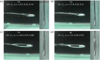
closest to each other. For example, figures 11 and 12 (case 2) and figures 17 and 18 (case 3) are steady-state phenomena for
$C_{q}$
closest to each other. For example, figures 11 and 12 (case 2) and figures 17 and 18 (case 3) are steady-state phenomena for
 $Fr=5.2$
, 7.8, 10.4, 13 with
$Fr=5.2$
, 7.8, 10.4, 13 with
 $C_{q}=0.24\pm 0.02$
and
$C_{q}=0.24\pm 0.02$
and
 $C_{q}=0.07$
, 0.15, 0.22, 0.37 with
$C_{q}=0.07$
, 0.15, 0.22, 0.37 with
 $Fr=5.2$
. Correspondingly, figures 24 and 25 (case 4) are steady-state phenomena for
$Fr=5.2$
. Correspondingly, figures 24 and 25 (case 4) are steady-state phenomena for
 $Fr=5.5$
, 7.3, 11, 12.9 with
$Fr=5.5$
, 7.3, 11, 12.9 with
 $C_{q}=0.23\pm 0.02$
and for
$C_{q}=0.23\pm 0.02$
and for
 $C_{q}=0.05$
, 0.15, 0.25, 0.34 with
$C_{q}=0.05$
, 0.15, 0.25, 0.34 with
 $Fr=5.5$
.
$Fr=5.5$
.

Figure 8. Side view observation of steady-state phenomena around a fully submerged moving body without a cavitator at various
 $Fr_{d}=V/(gd)^{1/2}$
(
$Fr_{d}=V/(gd)^{1/2}$
(
 $Fr_{d}=5.5$
, 7.3, 11, 12.9) for a
$Fr_{d}=5.5$
, 7.3, 11, 12.9) for a
 $C_{q,d}=0.23\pm 0.02$
; case 1 (
$C_{q,d}=0.23\pm 0.02$
; case 1 (
 $B=0$
,
$B=0$
,
 $h^{\ast }=0.5$
) in table 1.
$h^{\ast }=0.5$
) in table 1.
3.2.1 Case1: no cavitator and fully submerged
 $(B=0,h^{\ast }=0.5)$
Table 3 shows the operational table for the steady-state phenomena around a fully submerged moving body without a cavitator (case 1 in table 1) at various body speeds and ventilation flow rates. In the table, ‘x’ means no bubbles or cavities, ‘B’ means bubbly flow and ‘FC’ means a foamy cavity. In this case, no supercavitation is observed. Figure 8(a–d) shows steady-state phenomena at various
 $Fr_{d}$
(
$Fr_{d}$
(
 $Fr_{d}=5.5$
, 7.3, 11, 12.9) for a constant
$Fr_{d}=5.5$
, 7.3, 11, 12.9) for a constant
 $C_{q,d}=0.23\pm 0.02$
. All are foamy cavities. The foamy cavity is not transparent. In all cases, the resultant
$C_{q,d}=0.23\pm 0.02$
. All are foamy cavities. The foamy cavity is not transparent. In all cases, the resultant
 $\unicode[STIX]{x1D70E}_{c}$
is approximately 0.9. Figure 9(a–d) shows the steady-state phenomena at various
$\unicode[STIX]{x1D70E}_{c}$
is approximately 0.9. Figure 9(a–d) shows the steady-state phenomena at various
 $C_{q,d}$
(
$C_{q,d}$
(
 $C_{q,d}=0.05$
, 0.15, 0.25, 0.34) for a constant
$C_{q,d}=0.05$
, 0.15, 0.25, 0.34) for a constant
 $Fr_{d}=5.5$
. As
$Fr_{d}=5.5$
. As
 $C_{q,d}$
increases, the amount of a foamy cavity shed downstream increases, featuring more pointy air-filled bulge in front of the body nose. Corresponding to the operational table 3, for the physically meaningful dimensionless results, figure 10(a–c) shows the relationship between
$C_{q,d}$
increases, the amount of a foamy cavity shed downstream increases, featuring more pointy air-filled bulge in front of the body nose. Corresponding to the operational table 3, for the physically meaningful dimensionless results, figure 10(a–c) shows the relationship between
 $C_{q,d}$
and
$C_{q,d}$
and
 $Fr_{d}$
, between
$Fr_{d}$
, between
 $Fr_{d}$
and
$Fr_{d}$
and
 $\unicode[STIX]{x1D70E}_{c}$
and between
$\unicode[STIX]{x1D70E}_{c}$
and between
 $\unicode[STIX]{x1D70E}_{c}$
and
$\unicode[STIX]{x1D70E}_{c}$
and
 $C_{q,d}$
for the observed phenomena for case 1 (
$C_{q,d}$
for the observed phenomena for case 1 (
 $B=0$
,
$B=0$
,
 $h^{\ast }=0.5$
) in table 1. Overall, a relatively high
$h^{\ast }=0.5$
) in table 1. Overall, a relatively high
 $Fr_{d}$
favours a foamy cavity and a relatively low
$Fr_{d}$
favours a foamy cavity and a relatively low
 $Fr_{d}$
favours bubbly flow. In addition, as can be seen from figure 10(b), for a constant
$Fr_{d}$
favours bubbly flow. In addition, as can be seen from figure 10(b), for a constant
 $C_{q,d}$
, the cavitation number
$C_{q,d}$
, the cavitation number
 $\unicode[STIX]{x1D70E}_{c}$
slightly decreases as the
$\unicode[STIX]{x1D70E}_{c}$
slightly decreases as the
 $Fr_{d}$
increases, which can be attributed to an increased rate of air entrainment at the cavity trailing edge. By comparing the results of the present no-cavitator case (case 1) with those of cases with cavitators (cases 2–4) in later sections, we will see that the cavitator is indispensable in the generation of supercavitation.
$Fr_{d}$
increases, which can be attributed to an increased rate of air entrainment at the cavity trailing edge. By comparing the results of the present no-cavitator case (case 1) with those of cases with cavitators (cases 2–4) in later sections, we will see that the cavitator is indispensable in the generation of supercavitation.

Figure 9. Side view observation of steady-state phenomena around a fully submerged moving body without a cavitator at various
 $C_{q,d}$
(
$C_{q,d}$
(
 $C_{q,d}=0.05$
, 0.15, 0.25, 0.34) for a constant Froude number (
$C_{q,d}=0.05$
, 0.15, 0.25, 0.34) for a constant Froude number (
 $Fr_{d}=5.5$
); case 1 (
$Fr_{d}=5.5$
); case 1 (
 $B=0$
,
$B=0$
,
 $h^{\ast }=0.5$
) in table 1.
$h^{\ast }=0.5$
) in table 1.

Figure 10. Experimental relationship among dimensionless parameters in case 1 (
 $B=0$
,
$B=0$
,
 $h^{\ast }=0.5$
) in table 1. (a)
$h^{\ast }=0.5$
) in table 1. (a)
 $C_{q,d}$
versus
$C_{q,d}$
versus
 $Fr_{d}$
, (b)
$Fr_{d}$
, (b)
 $Fr_{d}$
versus
$Fr_{d}$
versus
 $\unicode[STIX]{x1D70E}_{c}$
, (c)
$\unicode[STIX]{x1D70E}_{c}$
, (c)
 $\unicode[STIX]{x1D70E}_{c}$
versus
$\unicode[STIX]{x1D70E}_{c}$
versus
 $C_{q,d}$
.
$C_{q,d}$
.
3.2.2 Case 2: Small blockage and fully submerged
$(B=1.5\,\%,h^{\ast }=0.5)$
Table 4. Operational table for the steady-state phenomena around a fully submerged moving body with a small blockage ratio (case 2 (
 $B=1.5\,\%$
,
$B=1.5\,\%$
,
 $h^{\ast }=0.5$
) in table 1) at various speeds (
$h^{\ast }=0.5$
) in table 1) at various speeds (
 $V$
:
$V$
:
 $\text{m}~\text{s}^{-1}$
) and ventilation flow rates (
$\text{m}~\text{s}^{-1}$
) and ventilation flow rates (
 $Q$
:
$Q$
:
 $\text{l}~\text{min}^{-1}$
). x: no bubbles or cavities, B: bubbly flow, FC: foamy cavity, TV: twin-vortex supercavity, RJ: reentrant-jet supercavity, HSF: half-supercavity with foamy cavity downstream.
$\text{l}~\text{min}^{-1}$
). x: no bubbles or cavities, B: bubbly flow, FC: foamy cavity, TV: twin-vortex supercavity, RJ: reentrant-jet supercavity, HSF: half-supercavity with foamy cavity downstream.

Figure 11. Side view and top view observations of steady-state phenomena around a fully submerged moving body with a small blockage ratio at various Froude numbers (
 $Fr=5.2$
, 7.8, 10.4, 13) for a constant flow rate coefficient (
$Fr=5.2$
, 7.8, 10.4, 13) for a constant flow rate coefficient (
 $C_{q}=0.24\pm 0.02$
); case 2 (
$C_{q}=0.24\pm 0.02$
); case 2 (
 $B=1.5\,\%$
,
$B=1.5\,\%$
,
 $h^{\ast }=0.5$
) in table 1.
$h^{\ast }=0.5$
) in table 1.

Figure 12. Side view and top view observations of steady-state phenomena around a fully submerged moving body with a small blockage ratio at various
 $C_{q}$
(
$C_{q}$
(
 $C_{q}=0.07$
, 0.15, 0.22, 0.37) for a constant Froude number (
$C_{q}=0.07$
, 0.15, 0.22, 0.37) for a constant Froude number (
 $Fr=5.2$
); case 2 (
$Fr=5.2$
); case 2 (
 $B=1.5\,\%$
,
$B=1.5\,\%$
,
 $h^{\ast }=0.5$
) in table 1.
$h^{\ast }=0.5$
) in table 1.

Figure 13. Air-entrainment coefficient (
 $C_{q}$
) versus Froude number (
$C_{q}$
) versus Froude number (
 $Fr$
) for various steady states for case 2 (
$Fr$
) for various steady states for case 2 (
 $B=1.5\,\%$
,
$B=1.5\,\%$
,
 $h^{\ast }=0.5$
) in table 1.
$h^{\ast }=0.5$
) in table 1.

Figure 14. Froude number (
 $Fr$
) versus cavitation number (
$Fr$
) versus cavitation number (
 $\unicode[STIX]{x1D70E}_{c}$
) for case 2 (
$\unicode[STIX]{x1D70E}_{c}$
) for case 2 (
 $B=1.5\,\%$
,
$B=1.5\,\%$
,
 $h^{\ast }=0.5$
) in table 1. (a) All states, (b) TV and RJ.
$h^{\ast }=0.5$
) in table 1. (a) All states, (b) TV and RJ.

Figure 15. Cavitation number (
 $\unicode[STIX]{x1D70E}_{c}$
) versus air-entrainment coefficient (
$\unicode[STIX]{x1D70E}_{c}$
) versus air-entrainment coefficient (
 $C_{q}$
) for case 2 (
$C_{q}$
) for case 2 (
 $B=1.5\,\%$
,
$B=1.5\,\%$
,
 $h^{\ast }=0.5$
) in table 1. (a) All states, (b) TV and RJ.
$h^{\ast }=0.5$
) in table 1. (a) All states, (b) TV and RJ.
Table 4 shows the operational table for the steady-state phenomena around a fully submerged moving body with a small blockage ratio (case 2 in table 1) at various body speeds and ventilation flow rates. In the table, ‘x’ means no bubbles or cavities, ‘B’ bubbly flow, ‘FC’ a foamy cavity, ‘TV’ a twin-vortex supercavity, ‘RJ’ a reentrant-jet supercavity and ‘HSF’ a half-supercavity with a foamy cavity downstream. In case 2 (
 $B=1.5\,\%$
,
$B=1.5\,\%$
,
 $h^{\ast }=0.5$
), two supercavitation phenomena (TV, RJ) are clearly observed. For example, figure 11 shows side and top view steady-state phenomena at various Froude numbers (
$h^{\ast }=0.5$
), two supercavitation phenomena (TV, RJ) are clearly observed. For example, figure 11 shows side and top view steady-state phenomena at various Froude numbers (
 $Fr=5.2$
, 7.8, 10.4, 13) for a constant flow rate coefficient (
$Fr=5.2$
, 7.8, 10.4, 13) for a constant flow rate coefficient (
 $C_{q}=0.24\pm 0.02$
). Compared to case 1, one can see the other side of the black tank wall through the cavity around the underwater body. At a low
$C_{q}=0.24\pm 0.02$
). Compared to case 1, one can see the other side of the black tank wall through the cavity around the underwater body. At a low
 $Fr$
(figure 11
a–c), the supercavity is not fore–aft symmetric. This is twin-vortex supercavitation. Two vortex tails of the supercavity are directed upwards. For a high
$Fr$
(figure 11
a–c), the supercavity is not fore–aft symmetric. This is twin-vortex supercavitation. Two vortex tails of the supercavity are directed upwards. For a high
 $Fr$
(figure 11
d), a rather smooth axisymmetric ellipsoidal supercavity can be seen and the supercavity has a tail with a reentrant-jet closure. Regardless of
$Fr$
(figure 11
d), a rather smooth axisymmetric ellipsoidal supercavity can be seen and the supercavity has a tail with a reentrant-jet closure. Regardless of
 $Fr$
-dependent differences, all the cases feature the smooth and axisymmetric nose of the cavity. The resultant
$Fr$
-dependent differences, all the cases feature the smooth and axisymmetric nose of the cavity. The resultant
 $\unicode[STIX]{x1D70E}_{c}$
are approximately 0.1 for the twin-vortex supercavities and the reentrant-jet supercavities. Compared to figure 11, figure 12 shows side and top view steady-state phenomena at various
$\unicode[STIX]{x1D70E}_{c}$
are approximately 0.1 for the twin-vortex supercavities and the reentrant-jet supercavities. Compared to figure 11, figure 12 shows side and top view steady-state phenomena at various
 $C_{q}$
(
$C_{q}$
(
 $C_{q}=0.07$
, 0.15, 0.22, 0.37) for a constant
$C_{q}=0.07$
, 0.15, 0.22, 0.37) for a constant
 $Fr=5.2$
. Two different states are observed; a foamy cavity (figure 12
a,b) and twin-vortex supercavities (figure 12
c,d). The resultant
$Fr=5.2$
. Two different states are observed; a foamy cavity (figure 12
a,b) and twin-vortex supercavities (figure 12
c,d). The resultant
 $\unicode[STIX]{x1D70E}_{c}$
values are 0.94 for the foamy cavity and 0.12 for the twin-vortex supercavities. Figures 11 and 12 correspond to some data for a constant
$\unicode[STIX]{x1D70E}_{c}$
values are 0.94 for the foamy cavity and 0.12 for the twin-vortex supercavities. Figures 11 and 12 correspond to some data for a constant
 $C_{q}=0.24\pm 0.02$
and for a constant
$C_{q}=0.24\pm 0.02$
and for a constant
 $Fr=5.2$
, respectively, in figures 13–15. In figures 13–15, all the relevant dimensionless results are summarized in terms of the relationships between
$Fr=5.2$
, respectively, in figures 13–15. In figures 13–15, all the relevant dimensionless results are summarized in terms of the relationships between
 $C_{q}$
and
$C_{q}$
and
 $Fr$
, between
$Fr$
, between
 $Fr$
and
$Fr$
and
 $\unicode[STIX]{x1D70E}_{c}$
and between
$\unicode[STIX]{x1D70E}_{c}$
and between
 $\unicode[STIX]{x1D70E}_{c}$
and
$\unicode[STIX]{x1D70E}_{c}$
and
 $C_{q}$
, respectively. From figures 13–15, a relatively high
$C_{q}$
, respectively. From figures 13–15, a relatively high
 $Fr$
(
$Fr$
(
 ${>}$
13) with
${>}$
13) with
 $C_{q}=0{-}1$
favours a reentrant-jet supercavity and a relatively low
$C_{q}=0{-}1$
favours a reentrant-jet supercavity and a relatively low
 $Fr$
(5–13) with
$Fr$
(5–13) with
 $C_{q}=0.1{-}3$
favours a twin-vortex supercavity. This trend may be compared with the most recent experimental results in a closed water tunnel by Karn et al. (Reference Karn, Arndt and Hong2016). With the same definitions of
$C_{q}=0.1{-}3$
favours a twin-vortex supercavity. This trend may be compared with the most recent experimental results in a closed water tunnel by Karn et al. (Reference Karn, Arndt and Hong2016). With the same definitions of
 $C_{q}$
and
$C_{q}$
and
 $Fr$
as those of the present work, for the least blockage ratio
$Fr$
as those of the present work, for the least blockage ratio
 $B=5\,\%$
in their work, a reentrant-jet supercavity occurs when both
$B=5\,\%$
in their work, a reentrant-jet supercavity occurs when both
 $C_{q}$
and
$C_{q}$
and
 $Fr$
are relatively low (
$Fr$
are relatively low (
 $C_{q}=0.02{-}0.04$
,
$C_{q}=0.02{-}0.04$
,
 $Fr=10{-}20$
), while a twin-vortex supercavity occurs when both
$Fr=10{-}20$
), while a twin-vortex supercavity occurs when both
 $C_{q}$
and
$C_{q}$
and
 $Fr$
are relatively high (
$Fr$
are relatively high (
 $C_{q}>0.2$
,
$C_{q}>0.2$
,
 $Fr>10{-}20$
). Karn et al. (Reference Karn, Arndt and Hong2016) posit that the closure mechanism is mainly determined by the pressure difference across the gas–water interface at the cavity closure.
$Fr>10{-}20$
). Karn et al. (Reference Karn, Arndt and Hong2016) posit that the closure mechanism is mainly determined by the pressure difference across the gas–water interface at the cavity closure.
 $$\begin{eqnarray}\displaystyle 2\frac{p_{out}-p_{in}}{\unicode[STIX]{x1D70C}V^{2}}=\widetilde{p}_{out}-\widetilde{p}_{in}=\unicode[STIX]{x0394}\widetilde{p}, & & \displaystyle\end{eqnarray}$$
where,
 $p_{in}$
and
$p_{in}$
and
 $p_{out}$
are pressures inside and outside the cavity at the closure. For the reentrant-jet (RJ) supercavity, the
$p_{out}$
are pressures inside and outside the cavity at the closure. For the reentrant-jet (RJ) supercavity, the
 $\unicode[STIX]{x0394}\widetilde{p}$
is dominated by the momentum of the reentrant water jet, while for a twin-vortex (TV) supercavity, such difference is much smaller, i.e.
$\unicode[STIX]{x0394}\widetilde{p}$
is dominated by the momentum of the reentrant water jet, while for a twin-vortex (TV) supercavity, such difference is much smaller, i.e.
 $\unicode[STIX]{x0394}\widetilde{p}_{RJ}\gg \unicode[STIX]{x0394}\widetilde{p}_{TV}$
. Therefore, according to (3.4), for fixed
$\unicode[STIX]{x0394}\widetilde{p}_{RJ}\gg \unicode[STIX]{x0394}\widetilde{p}_{TV}$
. Therefore, according to (3.4), for fixed
 $B$
and
$B$
and
 $Fr$
, high
$Fr$
, high
 $C_{q}$
implies an increase of cavity pressure, which results in higher
$C_{q}$
implies an increase of cavity pressure, which results in higher
 $\widetilde{p}_{in}$
. On the other hand,
$\widetilde{p}_{in}$
. On the other hand,
 $\widetilde{p}_{out}$
is little dependent on
$\widetilde{p}_{out}$
is little dependent on
 $C_{q}$
. Therefore, the resultant decrement in
$C_{q}$
. Therefore, the resultant decrement in
 $\unicode[STIX]{x0394}\widetilde{p}$
leads to a twin-vortex supercavity. At a high
$\unicode[STIX]{x0394}\widetilde{p}$
leads to a twin-vortex supercavity. At a high
 $Fr$
, however, the favoured formation of a twin-vortex supercavity cannot be readily explained using (3.4). In summary, in a closed environment (
$Fr$
, however, the favoured formation of a twin-vortex supercavity cannot be readily explained using (3.4). In summary, in a closed environment (
 $B=5\,\%$
), high
$B=5\,\%$
), high
 $C_{q}$
and
$C_{q}$
and
 $Fr$
favours a TV and low
$Fr$
favours a TV and low
 $C_{q}$
and
$C_{q}$
and
 $Fr$
favours an RJ. On the contrary, in a free-surface environment without any surface disturbance (
$Fr$
favours an RJ. On the contrary, in a free-surface environment without any surface disturbance (
 $B=1.5\,\%$
), a high
$B=1.5\,\%$
), a high
 $Fr$
favours an RJ and a low
$Fr$
favours an RJ and a low
 $Fr$
favours a TV, which is also different from Campbell & Hilborne’s (Reference Campbell and Hilborne1958) work. Their work was carried out in a circular free-surface water channel (water depth: 0.46 m, channel width: 0.91 m, submergence depth: 0.22 m) with disk-type cavitators (diameter: 0.013 m, 0.019 m, 0.025 m, blockage ratio
$Fr$
favours a TV, which is also different from Campbell & Hilborne’s (Reference Campbell and Hilborne1958) work. Their work was carried out in a circular free-surface water channel (water depth: 0.46 m, channel width: 0.91 m, submergence depth: 0.22 m) with disk-type cavitators (diameter: 0.013 m, 0.019 m, 0.025 m, blockage ratio
 $B=1.4\,\%$
, 2.1 %, 2.8 %,
$B=1.4\,\%$
, 2.1 %, 2.8 %,
 $h^{\ast }=0.47$
) although they did not consider the effect of the closeness of the free surface on the formation of the supercavity. Our case 2 (
$h^{\ast }=0.47$
) although they did not consider the effect of the closeness of the free surface on the formation of the supercavity. Our case 2 (
 $B=1.5\,\%$
,
$B=1.5\,\%$
,
 $h^{\ast }=0.5$
) is similar to their case (
$h^{\ast }=0.5$
) is similar to their case (
 $B=1.4\,\%$
,
$B=1.4\,\%$
,
 $h^{\ast }=0.47$
). They showed that an RJ supercavity occurs when
$h^{\ast }=0.47$
). They showed that an RJ supercavity occurs when
 $\unicode[STIX]{x1D70E}_{c}Fr>1$
and a TV supercavity occurs when
$\unicode[STIX]{x1D70E}_{c}Fr>1$
and a TV supercavity occurs when
 $\unicode[STIX]{x1D70E}_{c}Fr<1$
. This does not agree with our case 2. Figure 14(a,b) shows the relationship between
$\unicode[STIX]{x1D70E}_{c}Fr<1$
. This does not agree with our case 2. Figure 14(a,b) shows the relationship between
 $Fr$
and
$Fr$
and
 $\unicode[STIX]{x1D70E}_{c}$
for various
$\unicode[STIX]{x1D70E}_{c}$
for various
 $C_{q}$
. In figure 14(a), where all states are shown, one can see that the resultant
$C_{q}$
. In figure 14(a), where all states are shown, one can see that the resultant
 $\unicode[STIX]{x1D70E}_{c}$
for the B, FC and HSF states are approximately 0.9, while the resultant
$\unicode[STIX]{x1D70E}_{c}$
for the B, FC and HSF states are approximately 0.9, while the resultant
 $\unicode[STIX]{x1D70E}_{c}$
values for supercavitation (RJ and TV) are around 0.1. The large jump in the figure represents the state change from TV to HSF. The air flow rate coefficient
$\unicode[STIX]{x1D70E}_{c}$
values for supercavitation (RJ and TV) are around 0.1. The large jump in the figure represents the state change from TV to HSF. The air flow rate coefficient
 $C_{q}$
is just sufficient to make a TV supercavity for low
$C_{q}$
is just sufficient to make a TV supercavity for low
 $Fr=5.2{-}10.4$
, but is not sufficient to make an RJ supercavity for high
$Fr=5.2{-}10.4$
, but is not sufficient to make an RJ supercavity for high
 $Fr=13{-}18.2$
. Instead, the intermediate states HSF between TV and RJ are formed, which results in a high
$Fr=13{-}18.2$
. Instead, the intermediate states HSF between TV and RJ are formed, which results in a high
 $\unicode[STIX]{x1D70E}_{c}$
of around 0.9. Figure 15(a,b) shows the relationship between
$\unicode[STIX]{x1D70E}_{c}$
of around 0.9. Figure 15(a,b) shows the relationship between
 $C_{q}$
and
$C_{q}$
and
 $\unicode[STIX]{x1D70E}_{c}$
for various
$\unicode[STIX]{x1D70E}_{c}$
for various
 $Fr$
, for all states and the supercavity states of the RJ and TV, respectively. For a given
$Fr$
, for all states and the supercavity states of the RJ and TV, respectively. For a given
 $Fr$
, it is seen that a minimum cavitation number (
$Fr$
, it is seen that a minimum cavitation number (
 $\unicode[STIX]{x1D70E}_{c,min}$
) exists, regardless of the increase in the air flow rate (figure 15
b). The values of
$\unicode[STIX]{x1D70E}_{c,min}$
) exists, regardless of the increase in the air flow rate (figure 15
b). The values of
 $\unicode[STIX]{x1D70E}_{c,min}=0.064$
, 0.063, 0.055, 0.05, 0.049, 0.048 for
$\unicode[STIX]{x1D70E}_{c,min}=0.064$
, 0.063, 0.055, 0.05, 0.049, 0.048 for
 $Fr=5.2$
, 7.8, 10.4, 13, 15.6, 18.2, respectively. The curves are L-shaped. On the horizontal branch of the L-shaped curve (where
$Fr=5.2$
, 7.8, 10.4, 13, 15.6, 18.2, respectively. The curves are L-shaped. On the horizontal branch of the L-shaped curve (where
 $\unicode[STIX]{x1D70E}_{c}>\unicode[STIX]{x1D70E}_{c,min}$
), a small increase of
$\unicode[STIX]{x1D70E}_{c}>\unicode[STIX]{x1D70E}_{c,min}$
), a small increase of
 $Q$
(or
$Q$
(or
 $C_{q}$
) causes a large increase of the cavity pressure (
$C_{q}$
) causes a large increase of the cavity pressure (
 $p_{c}$
) (or a large decrease of
$p_{c}$
) (or a large decrease of
 $\unicode[STIX]{x1D70E}_{c}$
) and the length, width and height of a supercavity or an increase of the cavity volume. This is due to the difficulty of the air escaping from the cavity. On the other hand, on the vertical branch of the L-shaped curve (where
$\unicode[STIX]{x1D70E}_{c}$
) and the length, width and height of a supercavity or an increase of the cavity volume. This is due to the difficulty of the air escaping from the cavity. On the other hand, on the vertical branch of the L-shaped curve (where
 $\unicode[STIX]{x1D70E}_{c}\sim \unicode[STIX]{x1D70E}_{c,min}$
), further increments to the air-entrainment rate are simply balanced by an increase in the rate of air evacuation through the cavity’s trailing edge. At this point, the cavity pressure ceases to increase any further; the self-limiting behaviour establishes a minimum
$\unicode[STIX]{x1D70E}_{c}\sim \unicode[STIX]{x1D70E}_{c,min}$
), further increments to the air-entrainment rate are simply balanced by an increase in the rate of air evacuation through the cavity’s trailing edge. At this point, the cavity pressure ceases to increase any further; the self-limiting behaviour establishes a minimum
 $\unicode[STIX]{x1D70E}_{c}$
. All these can be confirmed from figure 16(a,b) where the normalized length (
$\unicode[STIX]{x1D70E}_{c}$
. All these can be confirmed from figure 16(a,b) where the normalized length (
 $l/d_{c}$
), height (
$l/d_{c}$
), height (
 $h/d_{c}$
) and width (
$h/d_{c}$
) and width (
 $w/d_{c}$
) of an RJ supercavity according to
$w/d_{c}$
) of an RJ supercavity according to
 $\unicode[STIX]{x1D70E}_{c}$
are shown for
$\unicode[STIX]{x1D70E}_{c}$
are shown for
 $Fr=13$
, 15.6 and 18.2. As shown in figure 16(a), for each
$Fr=13$
, 15.6 and 18.2. As shown in figure 16(a), for each
 $Fr$
, the cavity length increases as
$Fr$
, the cavity length increases as
 $\unicode[STIX]{x1D70E}_{c}$
decreases and becomes clustered near
$\unicode[STIX]{x1D70E}_{c}$
decreases and becomes clustered near
 $\unicode[STIX]{x1D70E}_{c,min}$
. Also, there is little difference for different
$\unicode[STIX]{x1D70E}_{c,min}$
. Also, there is little difference for different
 $Fr=13$
, 15.6 and 18.2 for
$Fr=13$
, 15.6 and 18.2 for
 $0.045<\unicode[STIX]{x1D70E}_{c}<0.12$
, in particular, there is a good collapse for
$0.045<\unicode[STIX]{x1D70E}_{c}<0.12$
, in particular, there is a good collapse for
 $0.045<\unicode[STIX]{x1D70E}_{c}<0.055$
and a small spread in the data for
$0.045<\unicode[STIX]{x1D70E}_{c}<0.055$
and a small spread in the data for
 $0.055<\unicode[STIX]{x1D70E}_{c}<0.12$
. The empirical formula, neglecting small
$0.055<\unicode[STIX]{x1D70E}_{c}<0.12$
. The empirical formula, neglecting small
 $Fr$
-dependent spread, between the cavity length (
$Fr$
-dependent spread, between the cavity length (
 $l/d_{c}$
) and
$l/d_{c}$
) and
 $\unicode[STIX]{x1D70E}_{c}$
is as follows;
$\unicode[STIX]{x1D70E}_{c}$
is as follows;
 $$\begin{eqnarray}\displaystyle \frac{l}{d_{c}}=\frac{0.8661}{\unicode[STIX]{x1D70E}_{c}^{1.18}}. & & \displaystyle\end{eqnarray}$$
For the cavity width and height, for each
 $Fr$
, similar trends according to
$Fr$
, similar trends according to
 $\unicode[STIX]{x1D70E}_{c}$
can be seen in figure 16(b). In addition, the cavity width is larger than the cavity height for each
$\unicode[STIX]{x1D70E}_{c}$
can be seen in figure 16(b). In addition, the cavity width is larger than the cavity height for each
 $Fr$
. Unlike length (
$Fr$
. Unlike length (
 $l/d_{c}$
) versus
$l/d_{c}$
) versus
 $\unicode[STIX]{x1D70E}_{c}$
in figure 16(a), the
$\unicode[STIX]{x1D70E}_{c}$
in figure 16(a), the
 $Fr$
-dependence can be clearly seen in width (
$Fr$
-dependence can be clearly seen in width (
 $w/d_{c}$
) versus
$w/d_{c}$
) versus
 $\unicode[STIX]{x1D70E}_{c}$
and height (
$\unicode[STIX]{x1D70E}_{c}$
and height (
 $h/d_{c}$
) versus
$h/d_{c}$
) versus
 $\unicode[STIX]{x1D70E}_{c}$
in figure 16(b). As the
$\unicode[STIX]{x1D70E}_{c}$
in figure 16(b). As the
 $Fr$
increases, the height and the width all increase, where the degree of the increment of the cavity height is relatively small compared to that of the cavity width. For
$Fr$
increases, the height and the width all increase, where the degree of the increment of the cavity height is relatively small compared to that of the cavity width. For
 $0.045<\unicode[STIX]{x1D70E}_{c}<0.07$
, the height data collapse while the width data do not. The empirical formulas for the cavity width (
$0.045<\unicode[STIX]{x1D70E}_{c}<0.07$
, the height data collapse while the width data do not. The empirical formulas for the cavity width (
 $w/d_{c}$
), height (
$w/d_{c}$
), height (
 $h/d_{c}$
) and
$h/d_{c}$
) and
 $\unicode[STIX]{x1D70E}_{c}$
are as follows:
$\unicode[STIX]{x1D70E}_{c}$
are as follows:
 $$\begin{eqnarray}\displaystyle & \displaystyle \frac{h}{d_{c}}=\left\{\begin{array}{@{}l@{}}\displaystyle \frac{1.3}{\unicode[STIX]{x1D70E}_{c}^{0.37}}~(Fr=13)\\ \displaystyle \frac{1.35}{\unicode[STIX]{x1D70E}_{c}^{0.36}}~(Fr=15.6)\\ \displaystyle \frac{1.52}{\unicode[STIX]{x1D70E}_{c}^{0.32}}~(Fr=18.2),\end{array}\right. & \displaystyle\end{eqnarray}$$
 $$\begin{eqnarray}\displaystyle & \displaystyle \frac{w}{d_{c}}=\left\{\begin{array}{@{}l@{}}\displaystyle \frac{1.54}{\unicode[STIX]{x1D70E}_{c}^{0.35}}~(Fr=13)\\ \displaystyle \frac{1.74}{\unicode[STIX]{x1D70E}_{c}^{0.32}}~(Fr=15.6)\\ \displaystyle \frac{1.83}{\unicode[STIX]{x1D70E}_{c}^{0.31}}~(Fr=18.2).\end{array}\right. & \displaystyle\end{eqnarray}$$
Also, in figure 16(a,b), we compare our results with existing analytical (Garabedian Reference Garabedian1955) and semi-empirical works (Reichardt Reference Reichardt1946; Waid Reference Waid1957). With the assumption of steady, inviscid, irrotational, incompressible fluid flow, Garabedian (Reference Garabedian1955) presented the following asymptotic analytical formulas for the dimensionless length and height (width) of a natural axisymmetric supercavity around a disk-type cavitator in an unbounded fluid;
 $$\begin{eqnarray}\displaystyle & \displaystyle \frac{l}{d_{c}}=\frac{\sqrt{0.827(1+\unicode[STIX]{x1D70E}_{c})}}{\unicode[STIX]{x1D70E}_{c}}\sqrt{\ln \frac{1}{\unicode[STIX]{x1D70E}_{c}}}, & \displaystyle\end{eqnarray}$$
 $$\begin{eqnarray}\displaystyle & \displaystyle \frac{h}{d_{c}}=\frac{w}{d_{c}}=\sqrt{\frac{0.827(1+\unicode[STIX]{x1D70E}_{c})}{\unicode[STIX]{x1D70E}_{c}}}. & \displaystyle\end{eqnarray}$$
Reichardt (Reference Reichardt1946) suggested the following semi-empirical formulas for the dimensionless length and height (width) of a natural axisymmetric supercavity around an axisymmetric body with a disk-type cavitator;
 $$\begin{eqnarray}\displaystyle & \displaystyle \frac{l}{d_{c}}=\sqrt{\frac{0.827(1+\unicode[STIX]{x1D70E}_{c})}{\unicode[STIX]{x1D70E}_{c}-0.132\unicode[STIX]{x1D70E}_{c}^{1.142857}}}\frac{\unicode[STIX]{x1D70E}_{c}+0.008}{\unicode[STIX]{x1D70E}_{c}(0.066+1.7\unicode[STIX]{x1D70E}_{c})}, & \displaystyle\end{eqnarray}$$
 $$\begin{eqnarray}\displaystyle & \displaystyle \frac{h}{d_{c}}=\frac{w}{d_{c}}=\sqrt{\frac{0.827(1+\unicode[STIX]{x1D70E}_{c})}{\unicode[STIX]{x1D70E}_{c}-0.132\unicode[STIX]{x1D70E}_{c}^{1.142857}}}. & \displaystyle\end{eqnarray}$$
Waid (Reference Waid1957) suggested the following semi-empirical formulas for the dimensionless length and height (width) of a ventilated supercavity around an axisymmetric body with a disk-type cavitator in a free-surface water tunnel, where the model was placed in the centre of the width and 12 inches above the bottom of the 20-by-20-inch test section. In our notation, the submergence depth is
 $h^{\ast }=8/20=0.4$
.
$h^{\ast }=8/20=0.4$
.
 $$\begin{eqnarray}\displaystyle & \displaystyle \frac{l}{d_{c}}=\frac{1.08}{\unicode[STIX]{x1D70E}_{c}^{1.118}}, & \displaystyle\end{eqnarray}$$
 $$\begin{eqnarray}\displaystyle & \displaystyle \frac{h}{d_{c}}=\frac{w}{d_{c}}=\frac{0.534}{\unicode[STIX]{x1D70E}_{c}^{0.568}}+1. & \displaystyle\end{eqnarray}$$
As shown in figure 16(a,b), the length and the height of a supercavity with a reentrant jet in the present work, for the most part, agree with those from the above three existing works (3.8)–(3.13). These three works agree with each other, showing a better agreement as
 $\unicode[STIX]{x1D70E}_{c}$
increases, even if the physical settings from which these equations are derived are all different. In particular, Waid’s (Reference Waid1957) work is closest to the present experiment although the dimensionless submergence depth is different;
$\unicode[STIX]{x1D70E}_{c}$
increases, even if the physical settings from which these equations are derived are all different. In particular, Waid’s (Reference Waid1957) work is closest to the present experiment although the dimensionless submergence depth is different;
 $h^{\ast }=0.5$
for our case 2 (and
$h^{\ast }=0.5$
for our case 2 (and
 $h^{\ast }=0.17$
for our case 3 in the next subsection § 3.2.3). The cavity length data are a little below Waid’s equation (3.12) and show a good agreement for
$h^{\ast }=0.17$
for our case 3 in the next subsection § 3.2.3). The cavity length data are a little below Waid’s equation (3.12) and show a good agreement for
 $0.045<\unicode[STIX]{x1D70E}_{c}<0.055$
. The cavity height data are spread but overlaid on (3.9), (3.11) and (3.13), showing good agreement for
$0.045<\unicode[STIX]{x1D70E}_{c}<0.055$
. The cavity height data are spread but overlaid on (3.9), (3.11) and (3.13), showing good agreement for
 $0.045<\unicode[STIX]{x1D70E}_{c}<0.055$
. Finally, all the cavity width data are well above (3.9), (3.11) and (3.13).
$0.045<\unicode[STIX]{x1D70E}_{c}<0.055$
. Finally, all the cavity width data are well above (3.9), (3.11) and (3.13).

Figure 16. Normalized length (
 $l/d_{c}$
), height (
$l/d_{c}$
), height (
 $h/d_{c}$
) and width (
$h/d_{c}$
) and width (
 $w/d_{c}$
) of the reentrant-jet supercavity according to
$w/d_{c}$
) of the reentrant-jet supercavity according to
 $\unicode[STIX]{x1D70E}_{c}$
, where
$\unicode[STIX]{x1D70E}_{c}$
, where
 $d_{c}$
is the diameter of the cavitator. (a) Normalized length, (b) normalized height and width; case 2 (
$d_{c}$
is the diameter of the cavitator. (a) Normalized length, (b) normalized height and width; case 2 (
 $B=1.5\,\%$
,
$B=1.5\,\%$
,
 $h^{\ast }=0.5$
) in table 1.
$h^{\ast }=0.5$
) in table 1.
3.2.3 Case 3: small blockage and shallowly submerged
$(B=1.5\,\%,h^{\ast }=0.17)$
Figure 17. Side view and top view observations of steady-state phenomena around a shallowly submerged moving body with a small blockage ratio at various Froude numbers (
 $Fr=5.2$
, 7.8, 10.4, 13) for a constant flow rate coefficient (
$Fr=5.2$
, 7.8, 10.4, 13) for a constant flow rate coefficient (
 $C_{q}=0.24\pm 0.02$
); case 3 (
$C_{q}=0.24\pm 0.02$
); case 3 (
 $B=1.5\,\%$
,
$B=1.5\,\%$
,
 $h^{\ast }=0.17$
) in table 1.
$h^{\ast }=0.17$
) in table 1.

Figure 18. Side view and top view observations of steady-state phenomena around a shallowly submerged moving body with a small blockage ratio at various
 $C_{q}$
(
$C_{q}$
(
 $C_{q}=0.07$
, 0.15, 0.22, 0.37) for a constant Froude number (
$C_{q}=0.07$
, 0.15, 0.22, 0.37) for a constant Froude number (
 $Fr=5.2$
); case 3 (
$Fr=5.2$
); case 3 (
 $B=1.5\,\%$
,
$B=1.5\,\%$
,
 $h^{\ast }=0.17$
) in table 1.
$h^{\ast }=0.17$
) in table 1.
Table 5. Operational table for the steady-state phenomena around a shallowly submerged moving body with a small blockage ratio (case 3 (
 $B=1.5\,\%$
,
$B=1.5\,\%$
,
 $h^{\ast }=0.17$
) in table 1) at various speeds (
$h^{\ast }=0.17$
) in table 1) at various speeds (
 $V$
:
$V$
:
 $\text{m}~\text{s}^{-1}$
) and ventilation flow rates (
$\text{m}~\text{s}^{-1}$
) and ventilation flow rates (
 $Q$
:
$Q$
:
 $\text{l}~\text{min}^{-1}$
). x: no bubbles or cavities, B: bubbly flow, FC: foamy cavity, TV: twin-vortex supercavity, RJ: reentrant-jet supercavity, HSF: half-supercavity with foamy cavity downstream.
$\text{l}~\text{min}^{-1}$
). x: no bubbles or cavities, B: bubbly flow, FC: foamy cavity, TV: twin-vortex supercavity, RJ: reentrant-jet supercavity, HSF: half-supercavity with foamy cavity downstream.


Figure 19. Air-entrainment coefficient (
 $C_{q}$
) versus Froude number (
$C_{q}$
) versus Froude number (
 $Fr$
) for various steady states for case 3 (
$Fr$
) for various steady states for case 3 (
 $B=1.5\,\%$
,
$B=1.5\,\%$
,
 $h^{\ast }=0.17$
) in table 1.
$h^{\ast }=0.17$
) in table 1.

Figure 20. Froude number (
 $Fr$
) versus cavitation number (
$Fr$
) versus cavitation number (
 $\unicode[STIX]{x1D70E}_{c}$
) for case 3 (
$\unicode[STIX]{x1D70E}_{c}$
) for case 3 (
 $B=1.5\,\%$
,
$B=1.5\,\%$
,
 $h^{\ast }=0.17$
) in table 1. (a) All states, (b) TV and RJ.
$h^{\ast }=0.17$
) in table 1. (a) All states, (b) TV and RJ.

Figure 21. Cavitation number (
 $\unicode[STIX]{x1D70E}_{c}$
) versus air-entrainment coefficient (
$\unicode[STIX]{x1D70E}_{c}$
) versus air-entrainment coefficient (
 $C_{q}$
) for case 3 (
$C_{q}$
) for case 3 (
 $B=1.5\,\%$
,
$B=1.5\,\%$
,
 $h^{\ast }=0.17$
) in table 1. (a) All states, (b) TV and RJ.
$h^{\ast }=0.17$
) in table 1. (a) All states, (b) TV and RJ.
To see the effect of the closeness of a body to the free surface on the supercavitation, we performed experiments for the shallowly submerged case with the same blockage ratio as case 2 which is fully submerged. Table 5 shows the operational table for the steady-state phenomena around a shallowly submerged moving body with a small blockage ratio (case 3 in table 1) at various body speeds and ventilation flow rates. It can be seen that there is little difference between table 4 (case 2) and table 5 (case 3) in terms of the categorization of steady-state phenomena. For example, the overall steady-state phenomena (figures 17 and 18) are similar to those in case 2 (figures 11 and 12) for the same set of (
 $Fr$
,
$Fr$
,
 $C_{q}$
). There are, however, differences in the detailed shapes of the cavity and the free surface. In case 3, the cavity shapes are not bottom–top symmetric and, also, the nearby free surface shows small-amplitude long waves due to the apparent shape of the supercavity around the moving body. The relationships among
$C_{q}$
). There are, however, differences in the detailed shapes of the cavity and the free surface. In case 3, the cavity shapes are not bottom–top symmetric and, also, the nearby free surface shows small-amplitude long waves due to the apparent shape of the supercavity around the moving body. The relationships among
 $Fr$
,
$Fr$
,
 $\unicode[STIX]{x1D70E}_{c}$
and
$\unicode[STIX]{x1D70E}_{c}$
and
 $C_{q}$
in case 3 (figures 19–21) are almost the same as those in case 2 (figures 13–15). In figures 19–21, all the relevant dimensionless results, including exemplary cases in figures 17 and 18, are summarized in terms of the relationships between
$C_{q}$
in case 3 (figures 19–21) are almost the same as those in case 2 (figures 13–15). In figures 19–21, all the relevant dimensionless results, including exemplary cases in figures 17 and 18, are summarized in terms of the relationships between
 $C_{q}$
and
$C_{q}$
and
 $Fr$
, between
$Fr$
, between
 $Fr$
and
$Fr$
and
 $\unicode[STIX]{x1D70E}_{c}$
and between
$\unicode[STIX]{x1D70E}_{c}$
and between
 $\unicode[STIX]{x1D70E}_{c}$
and
$\unicode[STIX]{x1D70E}_{c}$
and
 $C_{q}$
, respectively. In figure 19, as in case 2, a relatively high
$C_{q}$
, respectively. In figure 19, as in case 2, a relatively high
 $Fr$
(
$Fr$
(
 ${>}$
13) with
${>}$
13) with
 $C_{q}=0{-}1$
favours a reentrant-jet supercavity and a relatively low
$C_{q}=0{-}1$
favours a reentrant-jet supercavity and a relatively low
 $Fr$
(5–13) with
$Fr$
(5–13) with
 $C_{q}=0.1{-}3$
favours a twin-vortex supercavity. Figure 20(a,b) shows the relationship between
$C_{q}=0.1{-}3$
favours a twin-vortex supercavity. Figure 20(a,b) shows the relationship between
 $Fr$
and
$Fr$
and
 $\unicode[STIX]{x1D70E}_{c}$
for various
$\unicode[STIX]{x1D70E}_{c}$
for various
 $C_{q}$
. In figure 20(a) where all states are shown, one can see that the resultant
$C_{q}$
. In figure 20(a) where all states are shown, one can see that the resultant
 $\unicode[STIX]{x1D70E}_{c}$
for the B, FC and HSF states are approximately 0.9 while the resultant
$\unicode[STIX]{x1D70E}_{c}$
for the B, FC and HSF states are approximately 0.9 while the resultant
 $\unicode[STIX]{x1D70E}_{c}$
for supercavitation (RJ and TV) are approximately 0.1. The large jump in the figure represents a state change from a TV to a HSF. The air flow rate coefficient
$\unicode[STIX]{x1D70E}_{c}$
for supercavitation (RJ and TV) are approximately 0.1. The large jump in the figure represents a state change from a TV to a HSF. The air flow rate coefficient
 $C_{q}$
is just sufficient to make a TV supercavity for low
$C_{q}$
is just sufficient to make a TV supercavity for low
 $Fr=5.2{-}10.4$
, but is not sufficient to make an RJ supercavity for high
$Fr=5.2{-}10.4$
, but is not sufficient to make an RJ supercavity for high
 $Fr=13{-}18.2$
. Instead, the intermediate state HSF between a TV and RJ are formed, which results in a high
$Fr=13{-}18.2$
. Instead, the intermediate state HSF between a TV and RJ are formed, which results in a high
 $\unicode[STIX]{x1D70E}_{c}$
around 0.9. Figure 21(a,b) shows the relationship between
$\unicode[STIX]{x1D70E}_{c}$
around 0.9. Figure 21(a,b) shows the relationship between
 $C_{q}$
and
$C_{q}$
and
 $\unicode[STIX]{x1D70E}_{c}$
for various
$\unicode[STIX]{x1D70E}_{c}$
for various
 $Fr$
, for all states and the supercavity states of RJ and TV, respectively. For a given
$Fr$
, for all states and the supercavity states of RJ and TV, respectively. For a given
 $Fr$
, it is seen that a minimum cavitation number (
$Fr$
, it is seen that a minimum cavitation number (
 $\unicode[STIX]{x1D70E}_{c,min}$
) exists, regardless of an increase in the air flow rate (figure 21
b). The values are
$\unicode[STIX]{x1D70E}_{c,min}$
) exists, regardless of an increase in the air flow rate (figure 21
b). The values are
 $\unicode[STIX]{x1D70E}_{c,min}=0.063$
, 0.061, 0.053, 0.048, 0.047, 0.046 for
$\unicode[STIX]{x1D70E}_{c,min}=0.063$
, 0.061, 0.053, 0.048, 0.047, 0.046 for
 $Fr=5.2$
, 7.8, 10.4, 13, 15.6, 18.2, respectively. As shown in figure 22(a), for each
$Fr=5.2$
, 7.8, 10.4, 13, 15.6, 18.2, respectively. As shown in figure 22(a), for each
 $Fr$
, the cavity length increases as
$Fr$
, the cavity length increases as
 $\unicode[STIX]{x1D70E}_{c}$
decreases and becomes clustered near
$\unicode[STIX]{x1D70E}_{c}$
decreases and becomes clustered near
 $\unicode[STIX]{x1D70E}_{c,min}$
. Also, there is little difference for different
$\unicode[STIX]{x1D70E}_{c,min}$
. Also, there is little difference for different
 $Fr=13$
, 15.6 and 18.2 for
$Fr=13$
, 15.6 and 18.2 for
 $0.045<\unicode[STIX]{x1D70E}_{c}<0.12$
, in particular, a good collapse for
$0.045<\unicode[STIX]{x1D70E}_{c}<0.12$
, in particular, a good collapse for
 $0.045<\unicode[STIX]{x1D70E}_{c}<0.055$
and a small spread in the data for
$0.045<\unicode[STIX]{x1D70E}_{c}<0.055$
and a small spread in the data for
 $0.055<\unicode[STIX]{x1D70E}_{c}<0.12$
. Overall, the length data in case 3 (
$0.055<\unicode[STIX]{x1D70E}_{c}<0.12$
. Overall, the length data in case 3 (
 $h^{\ast }=0.17$
) are smaller than those in case 2 (
$h^{\ast }=0.17$
) are smaller than those in case 2 (
 $h^{\ast }=0.5$
) for the same
$h^{\ast }=0.5$
) for the same
 $\unicode[STIX]{x1D70E}_{c}$
. The proportional relationship between
$\unicode[STIX]{x1D70E}_{c}$
. The proportional relationship between
 $h^{\ast }$
and
$h^{\ast }$
and
 $l/d_{c}$
(or
$l/d_{c}$
(or
 $h_{s}$
and
$h_{s}$
and
 $l$
) can be explained by reference to figure 23(a,b). Figure 23(a) represents an RJ supercavity and the nearby free surface and figure 23(b) represents a streamline between the upper surface of an RJ supercavity and the free surface above the RJ supercavity. By applying Bernoulli’s theorem across the streamline in figure 23(a), one obtains the following equation:
$l$
) can be explained by reference to figure 23(a,b). Figure 23(a) represents an RJ supercavity and the nearby free surface and figure 23(b) represents a streamline between the upper surface of an RJ supercavity and the free surface above the RJ supercavity. By applying Bernoulli’s theorem across the streamline in figure 23(a), one obtains the following equation:
 $$\begin{eqnarray}\displaystyle \frac{p_{atm}-p_{c}}{h_{s}}\approx \unicode[STIX]{x1D70C}\frac{V^{2}}{R}. & & \displaystyle\end{eqnarray}$$
On the other hand, from figure 23(b), the radius of curvature
 $R$
of the streamline and the cavity length
$R$
of the streamline and the cavity length
 $l$
are geometrically related to each other as follows:
$l$
are geometrically related to each other as follows:
 $$\begin{eqnarray}\displaystyle l\approx R(2\unicode[STIX]{x1D703}). & & \displaystyle\end{eqnarray}$$
 $$\begin{eqnarray}\displaystyle \frac{p_{atm}-p_{c}}{h_{s}}\approx \unicode[STIX]{x1D70C}\frac{2\unicode[STIX]{x1D703}V^{2}}{l}. & & \displaystyle\end{eqnarray}$$
By rearranging (3.16) as follows,
 $$\begin{eqnarray}\displaystyle l\approx \frac{4\unicode[STIX]{x1D703}h_{s}}{2(p_{atm}-p_{c})/\unicode[STIX]{x1D70C}V^{2}}=\frac{4\unicode[STIX]{x1D703}h_{s}}{\unicode[STIX]{x1D70E}_{c}}. & & \displaystyle\end{eqnarray}$$
Thus, equation (3.17) explains the proportional relationship between
 $h_{s}$
and
$h_{s}$
and
 $l$
. In other words, for the same blockage ratio, the shallowly submerged case 3 results in a smaller cavity length compared to the fully submerged case 2. For the cavity width and height, for each
$l$
. In other words, for the same blockage ratio, the shallowly submerged case 3 results in a smaller cavity length compared to the fully submerged case 2. For the cavity width and height, for each
 $Fr$
, similar trends to the cavity length according to
$Fr$
, similar trends to the cavity length according to
 $\unicode[STIX]{x1D70E}_{c}$
can be seen in figure 22(b). In addition, the cavity width is larger than the cavity height for each
$\unicode[STIX]{x1D70E}_{c}$
can be seen in figure 22(b). In addition, the cavity width is larger than the cavity height for each
 $Fr$
. As with (
$Fr$
. As with (
 $l/d_{c}$
) versus
$l/d_{c}$
) versus
 $\unicode[STIX]{x1D70E}_{c}$
in figure 22(a), a very weak
$\unicode[STIX]{x1D70E}_{c}$
in figure 22(a), a very weak
 $Fr$
-dependence can be seen in width (
$Fr$
-dependence can be seen in width (
 $w/d_{c}$
) versus
$w/d_{c}$
) versus
 $\unicode[STIX]{x1D70E}_{c}$
and height (
$\unicode[STIX]{x1D70E}_{c}$
and height (
 $h/d_{c}$
) versus
$h/d_{c}$
) versus
 $\unicode[STIX]{x1D70E}_{c}$
in figure 22(b). In other words, the height and width data collapse regardless of the
$\unicode[STIX]{x1D70E}_{c}$
in figure 22(b). In other words, the height and width data collapse regardless of the
 $Fr$
, in particular, a better collapse for
$Fr$
, in particular, a better collapse for
 $0.045<\unicode[STIX]{x1D70E}_{c}<0.08$
. Overall, compared to case 2, the height and width data in case 3 collapse better and such that the height data for
$0.045<\unicode[STIX]{x1D70E}_{c}<0.08$
. Overall, compared to case 2, the height and width data in case 3 collapse better and such that the height data for
 $Fr=13$
, 15.6 approach those for
$Fr=13$
, 15.6 approach those for
 $Fr=18.2$
. In case 3, by making a long wave above the supercavity, the free surface plays the role of limiting the growth of the width and height of a supercavity, thus annihilating the effect of the
$Fr=18.2$
. In case 3, by making a long wave above the supercavity, the free surface plays the role of limiting the growth of the width and height of a supercavity, thus annihilating the effect of the
 $Fr$
. The empirical formulas for the cavity length (
$Fr$
. The empirical formulas for the cavity length (
 $l/d_{c}$
), width (
$l/d_{c}$
), width (
 $w/d_{c}$
) and height (
$w/d_{c}$
) and height (
 $h/d_{c}$
) are as follows
$h/d_{c}$
) are as follows
 $$\begin{eqnarray}\displaystyle & \displaystyle \frac{l}{d_{c}}=\frac{0.9513}{\unicode[STIX]{x1D70E}_{c}^{1.14}}, & \displaystyle\end{eqnarray}$$
 $$\begin{eqnarray}\displaystyle & \displaystyle \frac{h}{d_{c}}=\frac{1.4056}{\unicode[STIX]{x1D70E}_{c}^{0.36}}, & \displaystyle\end{eqnarray}$$
 $$\begin{eqnarray}\displaystyle & \displaystyle \frac{w}{d_{c}}=\frac{1.4984}{\unicode[STIX]{x1D70E}_{c}^{0.38}}. & \displaystyle\end{eqnarray}$$

Figure 22. Normalized length (
 $l/d_{c}$
), height (
$l/d_{c}$
), height (
 $h/d_{c}$
) and width (
$h/d_{c}$
) and width (
 $w/d_{c}$
) of the reentrant-jet supercavity according to
$w/d_{c}$
) of the reentrant-jet supercavity according to
 $\unicode[STIX]{x1D70E}_{c}$
, where
$\unicode[STIX]{x1D70E}_{c}$
, where
 $d_{c}$
is the diameter of the cavitator. (a) Normalized length, (b) normalized height and width; case 3 (
$d_{c}$
is the diameter of the cavitator. (a) Normalized length, (b) normalized height and width; case 3 (
 $B=1.5\,\%$
,
$B=1.5\,\%$
,
 $h^{\ast }=0.17$
) in table 1.
$h^{\ast }=0.17$
) in table 1.

Figure 23. Schematics for an RJ supercavity in a fluid with a free surface. (a) RJ supercavity and the nearby free surface, (b) a streamline between the upper surface of the RJ supercavity and the free surface above the RJ supercavity.
3.2.4 Case 4: Large blockage and fully submerged
$(B=3\,\%,h^{\ast }=0.5)$
Table 6. Operational table for the steady-state phenomena around a fully submerged moving body with a large blockage ratio (case 4 (
 $B=3\,\%$
,
$B=3\,\%$
,
 $h^{\ast }=0.5$
) in table 1) at various speeds (
$h^{\ast }=0.5$
) in table 1) at various speeds (
 $V$
:
$V$
:
 $\text{m}~\text{s}^{-1}$
) and ventilation flow rates (
$\text{m}~\text{s}^{-1}$
) and ventilation flow rates (
 $Q$
:
$Q$
:
 $\text{l}~\text{min}^{-1}$
). x: no bubbles or cavities, B: bubbly flow, FC: foamy cavity, TV: twin-vortex supercavity, RJ: reentrant-jet supercavity, HSV: half-supercavity with ring-type vortex shedding downstream, RJTV: double-layer supercavity with a reentrant-jet inside and twin vortices outside, TVTV: double-layer supercavity with twin vortices inside and twin vortices outside, RJRJ: double-layer supercavity a reentrant-jet inside and a reentrant-jet outside.
$\text{l}~\text{min}^{-1}$
). x: no bubbles or cavities, B: bubbly flow, FC: foamy cavity, TV: twin-vortex supercavity, RJ: reentrant-jet supercavity, HSV: half-supercavity with ring-type vortex shedding downstream, RJTV: double-layer supercavity with a reentrant-jet inside and twin vortices outside, TVTV: double-layer supercavity with twin vortices inside and twin vortices outside, RJRJ: double-layer supercavity a reentrant-jet inside and a reentrant-jet outside.


Figure 24. Side view and top view observations of steady-state phenomena around a fully submerged moving body with a large blockage ratio at various Froude numbers (
 $Fr=5.5$
, 7.3, 11, 12.9) for a constant flow rate coefficient (
$Fr=5.5$
, 7.3, 11, 12.9) for a constant flow rate coefficient (
 $C_{q}=0.23\pm 0.02$
); case 4 (
$C_{q}=0.23\pm 0.02$
); case 4 (
 $B=3\,\%$
,
$B=3\,\%$
,
 $h^{\ast }=0.5$
) in table 1.
$h^{\ast }=0.5$
) in table 1.

Figure 25. Side view and top view observations of steady-state phenomena around a fully submerged moving body with a large blockage ratio at various
 $C_{q}$
(
$C_{q}$
(
 $C_{q}=0.05$
, 0.15, 0.25, 0.34) for a constant Froude number (
$C_{q}=0.05$
, 0.15, 0.25, 0.34) for a constant Froude number (
 $Fr=5.5$
); case 4 (
$Fr=5.5$
); case 4 (
 $B=3\,\%$
,
$B=3\,\%$
,
 $h^{\ast }=0.5$
) in table 1.
$h^{\ast }=0.5$
) in table 1.
In case 4 (
 $B=3\,\%$
,
$B=3\,\%$
,
 $h^{\ast }=0.5$
), where the blockage ratio is twice that of case 2 and the submergence depth of the body is the same as that of case 2 (
$h^{\ast }=0.5$
), where the blockage ratio is twice that of case 2 and the submergence depth of the body is the same as that of case 2 (
 $B=1.5\,\%$
,
$B=1.5\,\%$
,
 $h^{\ast }=0.5$
), the overall flow phenomena are observed to be quite different from case 2, which can be seen from tables 4 and 6 by comparison. In table 6, ‘x’ means no bubbles or cavities, ‘B’ bubbles, ‘FC’ a foamy cavity, ‘TV’ a twin-vortex supercavity, ‘RJ’ a reentrant-jet supercavity, ‘HSV’ a half-supercavity with a ring-type vortex shedding downstream, ‘RJTV’ a double-layer supercavity with a reentrant jet inside and twin vortices outside (figure 25
d), ‘TVTV’ a double-layer supercavity with twin vortices inside and twin vortices outside (figure 24
b) and ‘RJRJ’ a double-layer supercavity with a reentrant jet inside and a reentrant jet outside (figure 24
c,d). Double-layer supercavities (RJTV, TVTV, RJRJ) in case 4 are not observed in either cases 2 or 3, and also were not observed in Campbell & Hilborne’s (Reference Campbell and Hilborne1958) work for similar conditions (
$h^{\ast }=0.5$
), the overall flow phenomena are observed to be quite different from case 2, which can be seen from tables 4 and 6 by comparison. In table 6, ‘x’ means no bubbles or cavities, ‘B’ bubbles, ‘FC’ a foamy cavity, ‘TV’ a twin-vortex supercavity, ‘RJ’ a reentrant-jet supercavity, ‘HSV’ a half-supercavity with a ring-type vortex shedding downstream, ‘RJTV’ a double-layer supercavity with a reentrant jet inside and twin vortices outside (figure 25
d), ‘TVTV’ a double-layer supercavity with twin vortices inside and twin vortices outside (figure 24
b) and ‘RJRJ’ a double-layer supercavity with a reentrant jet inside and a reentrant jet outside (figure 24
c,d). Double-layer supercavities (RJTV, TVTV, RJRJ) in case 4 are not observed in either cases 2 or 3, and also were not observed in Campbell & Hilborne’s (Reference Campbell and Hilborne1958) work for similar conditions (
 $B=2.8\,\%$
,
$B=2.8\,\%$
,
 $h^{\ast }=0.47$
). In figure 26, for a better understanding of the flow structures, photo-based illustrations for the RJTV, TVTV and RJRJ supercavities are drawn, along with their real photos. The outlines of the inner and outer layers are most clearly seen for RJTV supercavities and are less obvious, but discernible, in the upper part of the cavities for the TVTV and RJRJ supercavities. Both the inner and the outer layers are composed of air, and, between the two, there exists a foamy interface. The glassy regions of double-layer supercavities are less transparent than those of single-layer supercavities. In addition, apparently, double-layer supercavities have more foamy regions inside the cavities than single-layer supercavities. In figures 27–29, all the relevant dimensionless results, including exemplary cases in figures 24 and 25, are summarized in terms of the relationships between
$h^{\ast }=0.47$
). In figure 26, for a better understanding of the flow structures, photo-based illustrations for the RJTV, TVTV and RJRJ supercavities are drawn, along with their real photos. The outlines of the inner and outer layers are most clearly seen for RJTV supercavities and are less obvious, but discernible, in the upper part of the cavities for the TVTV and RJRJ supercavities. Both the inner and the outer layers are composed of air, and, between the two, there exists a foamy interface. The glassy regions of double-layer supercavities are less transparent than those of single-layer supercavities. In addition, apparently, double-layer supercavities have more foamy regions inside the cavities than single-layer supercavities. In figures 27–29, all the relevant dimensionless results, including exemplary cases in figures 24 and 25, are summarized in terms of the relationships between
 $C_{q}$
and
$C_{q}$
and
 $Fr$
, between
$Fr$
, between
 $Fr$
and
$Fr$
and
 $\unicode[STIX]{x1D70E}_{c}$
and between
$\unicode[STIX]{x1D70E}_{c}$
and between
 $\unicode[STIX]{x1D70E}_{c}$
and
$\unicode[STIX]{x1D70E}_{c}$
and
 $C_{q}$
, respectively. Figures 24 and 25 correspond to representative data for a constant flow rate
$C_{q}$
, respectively. Figures 24 and 25 correspond to representative data for a constant flow rate
 $C_{q}=0.23\pm 0.02$
and for a constant Froude number
$C_{q}=0.23\pm 0.02$
and for a constant Froude number
 $Fr=5.5$
, respectively, in figures 27–29. In figure 27, for
$Fr=5.5$
, respectively, in figures 27–29. In figure 27, for
 $Fr=1.8$
, all states (
$Fr=1.8$
, all states (
 $C_{q}$
: 0.03–0.74) are bubbly. For higher
$C_{q}$
: 0.03–0.74) are bubbly. For higher
 $Fr$
values, we successively observe different steady-state phenomena as
$Fr$
values, we successively observe different steady-state phenomena as
 $C_{q}$
increases at each
$C_{q}$
increases at each
 $Fr$
. For
$Fr$
. For
 $Fr=3.6$
, HSV (
$Fr=3.6$
, HSV (
 $C_{q}$
: 0.02–0.055)–TV (
$C_{q}$
: 0.02–0.055)–TV (
 $C_{q}$
: 0.07–0.46)–RJTV (
$C_{q}$
: 0.07–0.46)–RJTV (
 $C_{q}$
: 0.5–0.7). For
$C_{q}$
: 0.5–0.7). For
 $Fr=5.5$
, FC (
$Fr=5.5$
, FC (
 $C_{q}$
: 0.01)–HSV (
$C_{q}$
: 0.01)–HSV (
 $C_{q}$
: 0.02–0.05)–TV (
$C_{q}$
: 0.02–0.05)–TV (
 $C_{q}$
: 0.06–0.31)–RJTV (
$C_{q}$
: 0.06–0.31)–RJTV (
 $C_{q}$
: 0.34–0.46). For
$C_{q}$
: 0.34–0.46). For
 $Fr=7.3$
, FC (
$Fr=7.3$
, FC (
 $C_{q}$
: 0.01–0.14)–TV (
$C_{q}$
: 0.01–0.14)–TV (
 $C_{q}$
: 0.16–0.23)–TVTV (
$C_{q}$
: 0.16–0.23)–TVTV (
 $C_{q}$
: 0.25–0.35). For
$C_{q}$
: 0.25–0.35). For
 $Fr=9.2$
, FC (
$Fr=9.2$
, FC (
 $C_{q}$
: 0.007–0.18)–TVTV (
$C_{q}$
: 0.007–0.18)–TVTV (
 $C_{q}$
: 0.2–0.28). For
$C_{q}$
: 0.2–0.28). For
 $Fr=11$
, FC (
$Fr=11$
, FC (
 $C_{q}$
: 0.006–0.15)–RJRJ (
$C_{q}$
: 0.006–0.15)–RJRJ (
 $C_{q}$
: 0.17–0.23). For
$C_{q}$
: 0.17–0.23). For
 $Fr=12.9$
, FC (
$Fr=12.9$
, FC (
 $C_{q}$
: 0.005–0.13)–RJRJ (
$C_{q}$
: 0.005–0.13)–RJRJ (
 $C_{q}$
: 0.14–0.2). Figure 28(a,b) shows the relationship between
$C_{q}$
: 0.14–0.2). Figure 28(a,b) shows the relationship between
 $Fr$
and
$Fr$
and
 $\unicode[STIX]{x1D70E}_{c}$
for various
$\unicode[STIX]{x1D70E}_{c}$
for various
 $C_{q}$
. In figure 28(a) where all states are shown, one can see that the resultant
$C_{q}$
. In figure 28(a) where all states are shown, one can see that the resultant
 $\unicode[STIX]{x1D70E}_{c}$
for the non-supercavitating states (B, FC) are approximately 0.9 while the resultant
$\unicode[STIX]{x1D70E}_{c}$
for the non-supercavitating states (B, FC) are approximately 0.9 while the resultant
 $\unicode[STIX]{x1D70E}_{c}$
for supercavitation (TV, RJTV, TVTV, RJRJ) are around 0.1 and that for the HSV is around 0.25. The large jump in the figure represents a state change from a TV or RJTV or HSV to an FC. The air flow rate coefficient
$\unicode[STIX]{x1D70E}_{c}$
for supercavitation (TV, RJTV, TVTV, RJRJ) are around 0.1 and that for the HSV is around 0.25. The large jump in the figure represents a state change from a TV or RJTV or HSV to an FC. The air flow rate coefficient
 $C_{q}$
is just sufficient to make a TV or RJTV or HSV for low
$C_{q}$
is just sufficient to make a TV or RJTV or HSV for low
 $Fr=3.6{-}7.3$
, but is not sufficient to make an RJRJ or a TVTV supercavity for high
$Fr=3.6{-}7.3$
, but is not sufficient to make an RJRJ or a TVTV supercavity for high
 $Fr=9.2$
–12.9. Instead, an FC is formed, which results in a high
$Fr=9.2$
–12.9. Instead, an FC is formed, which results in a high
 $\unicode[STIX]{x1D70E}_{c}$
around 0.9. Figure 29(a,b) shows the relationship between
$\unicode[STIX]{x1D70E}_{c}$
around 0.9. Figure 29(a,b) shows the relationship between
 $C_{q}$
and
$C_{q}$
and
 $\unicode[STIX]{x1D70E}_{c}$
for various
$\unicode[STIX]{x1D70E}_{c}$
for various
 $Fr$
, for all states and the supercavity states of the HSV, TV, RJTV, TVTV and RJRJ, respectively. For a given
$Fr$
, for all states and the supercavity states of the HSV, TV, RJTV, TVTV and RJRJ, respectively. For a given
 $Fr$
, it is seen that a minimum cavitation number (
$Fr$
, it is seen that a minimum cavitation number (
 $\unicode[STIX]{x1D70E}_{c,min}$
) exists, regardless of an increase in
$\unicode[STIX]{x1D70E}_{c,min}$
) exists, regardless of an increase in
 $C_{q}$
(figure 29
b). The values are
$C_{q}$
(figure 29
b). The values are
 $\unicode[STIX]{x1D70E}_{c,min}=0.14$
, 0.13, 0.123, 0.12 for
$\unicode[STIX]{x1D70E}_{c,min}=0.14$
, 0.13, 0.123, 0.12 for
 $Fr=3.6$
, 5.5, 7.3, 9.2, respectively. In addition, with a variation of
$Fr=3.6$
, 5.5, 7.3, 9.2, respectively. In addition, with a variation of
 $C_{q}$
, there exists a minimum Froude number (
$C_{q}$
, there exists a minimum Froude number (
 $Fr=7.3$
) for supercavity states to be maintained without jumping to non-supercavitating states. In figure 30, the dimensionless length (
$Fr=7.3$
) for supercavity states to be maintained without jumping to non-supercavitating states. In figure 30, the dimensionless length (
 $l/d_{c}$
), height (
$l/d_{c}$
), height (
 $h/d_{c}$
) and width (
$h/d_{c}$
) and width (
 $w/d_{c}$
) of the RJRJ supercavity (inner-layer ellipsoid) with a reentrant jet are plotted according to
$w/d_{c}$
) of the RJRJ supercavity (inner-layer ellipsoid) with a reentrant jet are plotted according to
 $\unicode[STIX]{x1D70E}_{c}$
. To understand why the double-layer supercavities occur in case 4, let us consider figures 15(b) (case 2) and 29(b) (case 4), which are
$\unicode[STIX]{x1D70E}_{c}$
. To understand why the double-layer supercavities occur in case 4, let us consider figures 15(b) (case 2) and 29(b) (case 4), which are
 $C_{q}$
versus
$C_{q}$
versus
 $\unicode[STIX]{x1D70E}_{c}$
diagrams for several
$\unicode[STIX]{x1D70E}_{c}$
diagrams for several
 $Fr$
values. In figure 31, data from figures 15(b) and 29(b) are drawn altogether. It appears that case 4 data fill the
$Fr$
values. In figure 31, data from figures 15(b) and 29(b) are drawn altogether. It appears that case 4 data fill the
 $C_{q}$
versus
$C_{q}$
versus
 $\unicode[STIX]{x1D70E}_{c}$
diagram of case 2 in a complementary way. If there were no operational restrictions on
$\unicode[STIX]{x1D70E}_{c}$
diagram of case 2 in a complementary way. If there were no operational restrictions on
 $V$
,
$V$
,
 $Q$
or mechanical restrictions (e.g. the control of the submergence depth) such that the ranges of the relevant dimensionless numbers were comparable to each other, they would collapse onto the same curve although each point on the diagram may represent a different supercavity state. In other words, for the same
$Q$
or mechanical restrictions (e.g. the control of the submergence depth) such that the ranges of the relevant dimensionless numbers were comparable to each other, they would collapse onto the same curve although each point on the diagram may represent a different supercavity state. In other words, for the same
 $Fr$
and
$Fr$
and
 $C_{q}$
, the resultant supercavities in cases 2 and 4 will have the same value of
$C_{q}$
, the resultant supercavities in cases 2 and 4 will have the same value of
 $\unicode[STIX]{x1D70E}_{c}$
. The resultant supercavity shapes, however, could be different. The difference comes from the different blockage ratios
$\unicode[STIX]{x1D70E}_{c}$
. The resultant supercavity shapes, however, could be different. The difference comes from the different blockage ratios
 $B$
;
$B$
;
 $B=3\,\%$
of case 4 is twice that
$B=3\,\%$
of case 4 is twice that
 $B=1.5\,\%$
of case 2. Further, figure 32 shows both data from figures 16 (case 2) and 30 (case 4) together, which are the dimensionless cavity length, height and width data according to
$B=1.5\,\%$
of case 2. Further, figure 32 shows both data from figures 16 (case 2) and 30 (case 4) together, which are the dimensionless cavity length, height and width data according to
 $\unicode[STIX]{x1D70E}_{c}$
for the resultant RJ- and RJRJ-type supercavities, respectively; for the RJRJ-type supercavity, the inner-layer ellipsoid is considered. Again, data for cases 2 and 4 appear complementary to each other, and would collapse onto the same curve if the ranges of the relevant dimensionless numbers were comparable to each other. In other words, for the same
$\unicode[STIX]{x1D70E}_{c}$
for the resultant RJ- and RJRJ-type supercavities, respectively; for the RJRJ-type supercavity, the inner-layer ellipsoid is considered. Again, data for cases 2 and 4 appear complementary to each other, and would collapse onto the same curve if the ranges of the relevant dimensionless numbers were comparable to each other. In other words, for the same
 $\unicode[STIX]{x1D70E}_{c}$
, the larger blockage case 4 will admit a double-layer RJRJ supercavity instead of a single-layer RJ supercavity which may occur if there were no constraint on
$\unicode[STIX]{x1D70E}_{c}$
, the larger blockage case 4 will admit a double-layer RJRJ supercavity instead of a single-layer RJ supercavity which may occur if there were no constraint on
 $\unicode[STIX]{x1D70E}_{c}$
. In this particular case (a closed-shaped RJ supercavity), the resultant supercavities in cases 2 and 4 will have the same dimensionless ellipsoidal shapes. This reasoning can be checked from figure 44 in the Appendix, where the different supercavity shapes are shown for the similar values of (
$\unicode[STIX]{x1D70E}_{c}$
. In this particular case (a closed-shaped RJ supercavity), the resultant supercavities in cases 2 and 4 will have the same dimensionless ellipsoidal shapes. This reasoning can be checked from figure 44 in the Appendix, where the different supercavity shapes are shown for the similar values of (
 $Fr$
,
$Fr$
,
 $C_{q}$
,
$C_{q}$
,
 $\unicode[STIX]{x1D70E}_{c}$
) for cases 2 and 4.
$\unicode[STIX]{x1D70E}_{c}$
) for cases 2 and 4.

Figure 26. RJTV, TVTV and RJRJ supercavities (from top to bottom). (a) Photo shots, (b) illustrations based on photo shots.

Figure 27. Air-entrainment coefficient (
 $C_{q}$
) versus Froude number (
$C_{q}$
) versus Froude number (
 $Fr$
) for various steady states for case 4 (
$Fr$
) for various steady states for case 4 (
 $B=3\,\%$
,
$B=3\,\%$
,
 $h^{\ast }=0.5$
) in table 1.
$h^{\ast }=0.5$
) in table 1.

Figure 28. Froude number (
 $Fr$
) versus cavitation number (
$Fr$
) versus cavitation number (
 $\unicode[STIX]{x1D70E}_{c}$
) for case 4 (
$\unicode[STIX]{x1D70E}_{c}$
) for case 4 (
 $B=3\,\%$
,
$B=3\,\%$
,
 $h^{\ast }=0.5$
) in table 1. (a) All states, (b) TV, HSV, RJTV, TVTV, RJRJ.
$h^{\ast }=0.5$
) in table 1. (a) All states, (b) TV, HSV, RJTV, TVTV, RJRJ.

Figure 29. Cavitation number (
 $\unicode[STIX]{x1D70E}_{c}$
) versus air-entrainment coefficient (
$\unicode[STIX]{x1D70E}_{c}$
) versus air-entrainment coefficient (
 $C_{q}$
) for case 4 (
$C_{q}$
) for case 4 (
 $B=3\,\%$
,
$B=3\,\%$
,
 $h^{\ast }=0.5$
) in table 1. (a) All states, (b) TV, HSV, RJTV, TVTV, RJRJ.
$h^{\ast }=0.5$
) in table 1. (a) All states, (b) TV, HSV, RJTV, TVTV, RJRJ.

Figure 30. Normalized length (
 $l/d_{c}$
), height (
$l/d_{c}$
), height (
 $h/d_{c}$
) and width (
$h/d_{c}$
) and width (
 $w/d_{c}$
) of the supercavity according to
$w/d_{c}$
) of the supercavity according to
 $\unicode[STIX]{x1D70E}_{c}$
, where
$\unicode[STIX]{x1D70E}_{c}$
, where
 $d_{c}$
is the diameter of the cavitator. (a) Normalized length, (b) normalized height and width; case 4 (
$d_{c}$
is the diameter of the cavitator. (a) Normalized length, (b) normalized height and width; case 4 (
 $B=3\,\%$
,
$B=3\,\%$
,
 $h^{\ast }=0.5$
) in table 1.
$h^{\ast }=0.5$
) in table 1.

Figure 31. Cavitation number (
 $\unicode[STIX]{x1D70E}_{c}$
) versus air-entrainment coefficient (
$\unicode[STIX]{x1D70E}_{c}$
) versus air-entrainment coefficient (
 $C_{q}$
) for case 2 (
$C_{q}$
) for case 2 (
 $B=1.5\,\%$
,
$B=1.5\,\%$
,
 $h^{\ast }=0.5$
) and case 4 (
$h^{\ast }=0.5$
) and case 4 (
 $B=3\,\%$
,
$B=3\,\%$
,
 $h^{\ast }=0.5$
) in table 1.
$h^{\ast }=0.5$
) in table 1.

Figure 32. Normalized length (
 $l/d_{c}$
), height (
$l/d_{c}$
), height (
 $h/d_{c}$
) and width (
$h/d_{c}$
) and width (
 $w/d_{c}$
) of the reentrant-jet supercavity according to
$w/d_{c}$
) of the reentrant-jet supercavity according to
 $\unicode[STIX]{x1D70E}_{c}$
for case 2 (
$\unicode[STIX]{x1D70E}_{c}$
for case 2 (
 $B=1.5\,\%$
,
$B=1.5\,\%$
,
 $h^{\ast }=0.5$
) and case 4 (
$h^{\ast }=0.5$
) and case 4 (
 $B=3\,\%$
,
$B=3\,\%$
,
 $h^{\ast }=0.5$
) in table 1. (a) Normalized length, (b) normalized height and width.
$h^{\ast }=0.5$
) in table 1. (a) Normalized length, (b) normalized height and width.
4 Drag measurement

Figure 33. Measurement of power consumption (
 $P=\text{voltage}\times \text{current}$
).
$P=\text{voltage}\times \text{current}$
).

Figure 34. Measurement of power consumption required to move the carriage system with a speed
 $V$
. (a) With a sphere, (b) without a sphere.
$V$
. (a) With a sphere, (b) without a sphere.

Figure 35. Frontal-area-based drag coefficient
 $C_{d}=F_{D}/[(1/2)\unicode[STIX]{x1D70C}V^{2}(\unicode[STIX]{x03C0}/4d_{s}^{2})]$
according to the diameter-based Reynolds number
$C_{d}=F_{D}/[(1/2)\unicode[STIX]{x1D70C}V^{2}(\unicode[STIX]{x03C0}/4d_{s}^{2})]$
according to the diameter-based Reynolds number
 $Re_{d_{s}}=Vd_{s}/\unicode[STIX]{x1D708}$
(
$Re_{d_{s}}=Vd_{s}/\unicode[STIX]{x1D708}$
(
 $\unicode[STIX]{x1D708}$
: kinematic viscosity of the fluid). The solid curve comes from Goldstein (Reference Goldstein1938).
$\unicode[STIX]{x1D708}$
: kinematic viscosity of the fluid). The solid curve comes from Goldstein (Reference Goldstein1938).
In the experiment, the drag force (
 $F_{D}$
) for a moving body with a speed
$F_{D}$
) for a moving body with a speed
 $V$
is obtained indirectly from the power consumption
$V$
is obtained indirectly from the power consumption
 $P$
for the RC-car run;
$P$
for the RC-car run;
 $F_{D}=P/V$
. The power consumption (
$F_{D}=P/V$
. The power consumption (
 $P=\text{voltage}\times \text{current}$
) is measured using a voltage sensor (Quanum TC9400, Operation range: 0–45 V,
$P=\text{voltage}\times \text{current}$
) is measured using a voltage sensor (Quanum TC9400, Operation range: 0–45 V,
 $\text{error}<\pm 1\,\%$
) and a current sensor (Quanum ACS755 LCB-100, operation range: 0–100 A,
$\text{error}<\pm 1\,\%$
) and a current sensor (Quanum ACS755 LCB-100, operation range: 0–100 A,
 $\text{error}<\pm 1\,\%$
) which are schematically shown in figure 33. In the figure, the RC car is represented by the driving motor (M). Before the measurement of drag forces of the moving body in cases 1–4, we performed a preliminary test for the drag coefficients of moving spheres in water or air. In figure 34, as a first step, we measure the power consumption (
$\text{error}<\pm 1\,\%$
) which are schematically shown in figure 33. In the figure, the RC car is represented by the driving motor (M). Before the measurement of drag forces of the moving body in cases 1–4, we performed a preliminary test for the drag coefficients of moving spheres in water or air. In figure 34, as a first step, we measure the power consumption (
 $P_{1}$
) required to move the sphere-attached carriage system with a speed
$P_{1}$
) required to move the sphere-attached carriage system with a speed
 $V$
in water or air. Next, we measure the power consumption (
$V$
in water or air. Next, we measure the power consumption (
 $P_{2}$
) required to move the sphere-removed carriage system with the same speed
$P_{2}$
) required to move the sphere-removed carriage system with the same speed
 $V$
in water or air. As already stated in § 2 (describing the experimental set-up), the support structure (cylindrical rod with a diameter of 10 mm) is C-shaped or positioned downstream so that there will be little influence on the flow upstream where a body exists. However, there will be a contribution to the drag force due to the vortex shedding. All the frictional and pressure drags, including this vortex-induced drag force during the translational motion with a speed
$V$
in water or air. As already stated in § 2 (describing the experimental set-up), the support structure (cylindrical rod with a diameter of 10 mm) is C-shaped or positioned downstream so that there will be little influence on the flow upstream where a body exists. However, there will be a contribution to the drag force due to the vortex shedding. All the frictional and pressure drags, including this vortex-induced drag force during the translational motion with a speed
 $V$
, are collectively and completely considered in the power consumption. Then, the drag force
$V$
, are collectively and completely considered in the power consumption. Then, the drag force
 $F_{D}$
of the sphere only can be obtained as follows;
$F_{D}$
of the sphere only can be obtained as follows;
 $$\begin{eqnarray}\displaystyle F_{D}=\frac{P_{1}-P_{2}}{V}. & & \displaystyle\end{eqnarray}$$
Then, if the diameter of the moving sphere is
 $d_{s}$
in the fluid (density:
$d_{s}$
in the fluid (density:
 $\unicode[STIX]{x1D70C}$
), the frontal-area-based drag coefficient
$\unicode[STIX]{x1D70C}$
), the frontal-area-based drag coefficient
 $C_{d}$
can be obtained as follows;
$C_{d}$
can be obtained as follows;
 $$\begin{eqnarray}\displaystyle C_{d}=\frac{F_{D}}{\displaystyle \frac{1}{2}\unicode[STIX]{x1D70C}V^{2}\left(\frac{\unicode[STIX]{x03C0}}{4}d_{s}^{2}\right)}. & & \displaystyle\end{eqnarray}$$
The resultant
 $C_{d}$
obtained using (4.1) and (4.2) is shown in figure 35, according to the diameter-based Reynolds number
$C_{d}$
obtained using (4.1) and (4.2) is shown in figure 35, according to the diameter-based Reynolds number
 $Re_{d_{s}}=Vd_{s}/\unicode[STIX]{x1D708}$
(
$Re_{d_{s}}=Vd_{s}/\unicode[STIX]{x1D708}$
(
 $\unicode[STIX]{x1D708}$
: kinematic viscosity of the fluid). For comparison, figure 35 (solid curve) shows the well-known experimental results for the identically defined
$\unicode[STIX]{x1D708}$
: kinematic viscosity of the fluid). For comparison, figure 35 (solid curve) shows the well-known experimental results for the identically defined
 $C_{d}$
(Goldstein Reference Goldstein1938). As shown, for the
$C_{d}$
(Goldstein Reference Goldstein1938). As shown, for the
 $Re_{d_{s}}$
range in the present experimental setting (
$Re_{d_{s}}$
range in the present experimental setting (
 $70\,000<Re_{d_{s}}<210\,000$
), they agree with each other very well. In a similar way to the preliminary sphere test, we measured the drag coefficient
$70\,000<Re_{d_{s}}<210\,000$
), they agree with each other very well. In a similar way to the preliminary sphere test, we measured the drag coefficient
 $C_{d}$
for cases 1–4. For example, for a moving body with a reentrant-jet supercavity, we performed four separate tests to obtain the drag coefficients (figure 36
a–c). First, we measured the power consumption
$C_{d}$
for cases 1–4. For example, for a moving body with a reentrant-jet supercavity, we performed four separate tests to obtain the drag coefficients (figure 36
a–c). First, we measured the power consumption
 $P_{1}$
for moving the whole carriage system with a body attached, around which a reentrant-jet supercavity is formed (figure 36
b) in water:
$P_{1}$
for moving the whole carriage system with a body attached, around which a reentrant-jet supercavity is formed (figure 36
b) in water:
 $$\begin{eqnarray}\displaystyle P_{1}=P_{RC\,car}+P_{c\text{-}shaped\,rod}+P_{body\,with\,a\,supercavity}. & & \displaystyle\end{eqnarray}$$
Next, after removing the supercavitating part (body plus rod), we performed the running test in water and measured the power consumption
 $P_{2}$
(figure 36
b):
$P_{2}$
(figure 36
b):
 $$\begin{eqnarray}\displaystyle P_{2}=P_{RC\,car}+P_{cut\,c\text{-}shaped\,rod,\,water}. & & \displaystyle\end{eqnarray}$$
By subtracting (4.4) from (4.3),
 $P_{1}-P_{2}$
, we can calculate the power consumption for the body plus the supercavity plus the rod inside the supercavity (figure 36
b). To remove the effect of the rod inside the air-filled supercavity, we performed the running test without a body in the air as shown in figure 36(c) and measured the power consumption
$P_{1}-P_{2}$
, we can calculate the power consumption for the body plus the supercavity plus the rod inside the supercavity (figure 36
b). To remove the effect of the rod inside the air-filled supercavity, we performed the running test without a body in the air as shown in figure 36(c) and measured the power consumption
 $P_{3}$
(figure 36
c)
$P_{3}$
(figure 36
c)
 $$\begin{eqnarray}\displaystyle P_{3}=P_{RC\,car}+P_{c\text{-}shaped\,rod,\,air}. & & \displaystyle\end{eqnarray}$$
Then, similar to (4.4), but in the air, we performed the running test and measured the power consumption
 $P_{4}$
(figure 36
c)
$P_{4}$
(figure 36
c)
 $$\begin{eqnarray}\displaystyle P_{4}=P_{RC\,car}+P_{cut\,c\text{-}shaped\,rod,\,air}. & & \displaystyle\end{eqnarray}$$
By subtracting (4.6) from (4.5),
 $P_{3}-P_{4}$
, we can calculate the power consumption for the rod inside the supercavity (figure 36
c). From (4.3)–(4.6), for the moving body (speed:
$P_{3}-P_{4}$
, we can calculate the power consumption for the rod inside the supercavity (figure 36
c). From (4.3)–(4.6), for the moving body (speed:
 $V$
) with a supercavity (figure 36
a), the required power consumption (
$V$
) with a supercavity (figure 36
a), the required power consumption (
 $P$
) will be
$P$
) will be
 $$\begin{eqnarray}\displaystyle P=P_{1}-P_{2}-(P_{3}-P_{4}). & & \displaystyle\end{eqnarray}$$
Then, the drag force
 $F_{D}$
can be obtained as follows:
$F_{D}$
can be obtained as follows:
 $$\begin{eqnarray}\displaystyle F_{D}=\frac{P}{V}. & & \displaystyle\end{eqnarray}$$
Finally, the body-frontal-area-based drag coefficient is calculated:
 $$\begin{eqnarray}\displaystyle C_{d}=\frac{F_{D}}{\displaystyle \frac{1}{2}\unicode[STIX]{x1D70C}V^{2}\left(\frac{\unicode[STIX]{x03C0}}{4}d^{2}\right)}. & & \displaystyle\end{eqnarray}$$
In this way, all the drag coefficients
 $C_{d}$
for cases 1–4 are obtained, and the results are summarized in figures 37 and 38. In figure 37(a–d), the cavitation number
$C_{d}$
for cases 1–4 are obtained, and the results are summarized in figures 37 and 38. In figure 37(a–d), the cavitation number
 $\unicode[STIX]{x1D70E}_{c}$
versus drag coefficient
$\unicode[STIX]{x1D70E}_{c}$
versus drag coefficient
 $C_{d}$
is shown depending on the Froude number
$C_{d}$
is shown depending on the Froude number
 $Fr_{d}$
(case 1) or
$Fr_{d}$
(case 1) or
 $Fr$
(cases 2–4), respectively. The vertical axes have been rescaled to accentuate the minute variation in
$Fr$
(cases 2–4), respectively. The vertical axes have been rescaled to accentuate the minute variation in
 $C_{d}$
, all of which lie within about 4 % of the mean value for each case. In figure 38, the drag coefficient
$C_{d}$
, all of which lie within about 4 % of the mean value for each case. In figure 38, the drag coefficient
 $C_{d}$
in figure 37(a–d) is replotted according to the body-diameter-based Reynolds number
$C_{d}$
in figure 37(a–d) is replotted according to the body-diameter-based Reynolds number
 $Re_{d}$
for all cases 1–4. For a non-supercavitating body with a cavitator (cases 2–4), the drag coefficient
$Re_{d}$
for all cases 1–4. For a non-supercavitating body with a cavitator (cases 2–4), the drag coefficient
 $C_{d}$
is approximately 1.15. Note that this number is very close to the well-known
$C_{d}$
is approximately 1.15. Note that this number is very close to the well-known
 $C_{d}=1.17$
of the disk (White Reference White1999). For a non-supercavitating body without a cavitator (case 1), the drag coefficient
$C_{d}=1.17$
of the disk (White Reference White1999). For a non-supercavitating body without a cavitator (case 1), the drag coefficient
 $C_{d}$
is approximately 0.4. For a supercavitating body (TV, RJ, RJTV, TVTV, RJRJ) in cases 2–4, the drag coefficient
$C_{d}$
is approximately 0.4. For a supercavitating body (TV, RJ, RJTV, TVTV, RJRJ) in cases 2–4, the drag coefficient
 $C_{d}$
is approximately 0.11. By comparing the case where
$C_{d}$
is approximately 0.11. By comparing the case where
 $C_{d}$
is approximately 0.4 (a non-supercavitating body without a cavitator) and the case where
$C_{d}$
is approximately 0.4 (a non-supercavitating body without a cavitator) and the case where
 $C_{d}$
is approximately 1.15 (a non-supercavitating body with a cavitator), in the case of no supercavity, we see that the existence of the cavitator has a negative effect on the drag reduction. However, as seen from the case where
$C_{d}$
is approximately 1.15 (a non-supercavitating body with a cavitator), in the case of no supercavity, we see that the existence of the cavitator has a negative effect on the drag reduction. However, as seen from the case where
 $C_{d}$
is approximately 0.11 (a supercavitating body with TV, RJ, RJTV, TVTV, RJRJ supercavities), the just-mentioned negative effect of a cavitator is noticeably compensated by the generation of a supercavity, which plays a significant role by reducing
$C_{d}$
is approximately 0.11 (a supercavitating body with TV, RJ, RJTV, TVTV, RJRJ supercavities), the just-mentioned negative effect of a cavitator is noticeably compensated by the generation of a supercavity, which plays a significant role by reducing
 $C_{d}$
by approximately 73 % (
$C_{d}$
by approximately 73 % (
 $=(0.4-0.11)/0.4$
) compared to the case where
$=(0.4-0.11)/0.4$
) compared to the case where
 $C_{d}$
is approximately 0.4, and approximately 90 % (
$C_{d}$
is approximately 0.4, and approximately 90 % (
 $=\,(1.15-0.11)/1.15$
) compared to the case where
$=\,(1.15-0.11)/1.15$
) compared to the case where
 $C_{d}$
is approximately 1.15.
$C_{d}$
is approximately 1.15.

Figure 36. Schematics for the calculation of power consumption of a supercavitating moving body with speed
 $V$
. (a) A supercavitating moving body, (b) a supercavitating moving body plus a cut rod inside the supercavity, (c) cut rod inside the supercavity.
$V$
. (a) A supercavitating moving body, (b) a supercavitating moving body plus a cut rod inside the supercavity, (c) cut rod inside the supercavity.

Figure 37. Drag coefficient
 $C_{d}$
of moving bodies (cases 1–4) according to the cavitation number
$C_{d}$
of moving bodies (cases 1–4) according to the cavitation number
 $\unicode[STIX]{x1D70E}_{c}$
and the Froude number
$\unicode[STIX]{x1D70E}_{c}$
and the Froude number
 $Fr_{d}$
(case 1) or
$Fr_{d}$
(case 1) or
 $Fr$
(cases 2–4).
$Fr$
(cases 2–4).

Figure 38. Drag coefficient
 $C_{d}$
of moving bodies (cases 1–4) according to the body-diameter-based Reynolds number
$C_{d}$
of moving bodies (cases 1–4) according to the body-diameter-based Reynolds number
 $Re_{d}$
. (a) Overall
$Re_{d}$
. (a) Overall
 $Re_{d}$
versus
$Re_{d}$
versus
 $C_{d}$
diagram, (b)
$C_{d}$
diagram, (b)
 $Re_{d}$
versus
$Re_{d}$
versus
 $C_{d}$
diagram near
$C_{d}$
diagram near
 $C_{d}=1.15$
, (c)
$C_{d}=1.15$
, (c)
 $Re_{d}$
versus
$Re_{d}$
versus
 $C_{d}$
diagram near
$C_{d}$
diagram near
 $C_{d}=0.4$
, (d)
$C_{d}=0.4$
, (d)
 $Re_{d}$
versus
$Re_{d}$
versus
 $C_{d}$
diagram near
$C_{d}$
diagram near
 $C_{d}=0.11$
.
$C_{d}=0.11$
.

Figure 39. A control volume for the analysis of the drag. The control volume is composed of a surface at upstream infinity (
 $S_{u}$
), a stream tube at infinity, the annular surface (
$S_{u}$
), a stream tube at infinity, the annular surface (
 $S$
) at the location of the maximum cavity height and the cross-sectional surface (
$S$
) at the location of the maximum cavity height and the cross-sectional surface (
 $S_{c}$
) at the location of the maximum cavity height.
$S_{c}$
) at the location of the maximum cavity height.
To analyse the experimental results of the drag measurement, let us consider the control volume in figure 39, where the reference frame is attached to the moving body. The control volume is composed of a surface at upstream infinity (
 $S_{u}$
), a stream tube at infinity, the annular surface (
$S_{u}$
), a stream tube at infinity, the annular surface (
 $S$
) at the location of the maximum cavity height and the cross-sectional surface (
$S$
) at the location of the maximum cavity height and the cross-sectional surface (
 $S_{c}$
) at the location of the maximum cavity height. The following analysis is based on the work of Franc & Michel (Reference Franc and Michel2004). From the mass conservation,
$S_{c}$
) at the location of the maximum cavity height. The following analysis is based on the work of Franc & Michel (Reference Franc and Michel2004). From the mass conservation,
 $$\begin{eqnarray}\displaystyle \unicode[STIX]{x1D70C}VS_{u}=\int _{s}\unicode[STIX]{x1D70C}U_{a}\,\text{d}A. & & \displaystyle\end{eqnarray}$$
From the linear momentum theorem,
 $$\begin{eqnarray}\displaystyle F_{D}-p_{\infty }(S+S_{c})+p_{c}S_{c}+\int _{s}p\,\text{d}A=\unicode[STIX]{x1D70C}V^{2}S_{u}-\int _{s}\unicode[STIX]{x1D70C}U_{a}^{2}\,\text{d}A, & & \displaystyle\end{eqnarray}$$
where
 $F_{D}$
is the drag force to the cavitating body. By combining (4.10) and (4.11),
$F_{D}$
is the drag force to the cavitating body. By combining (4.10) and (4.11),
 $$\begin{eqnarray}\displaystyle F_{D}=(p_{\infty }-p_{c})S_{c}-\int _{s}(p-p_{\infty })\,\text{d}A+\int _{s}\unicode[STIX]{x1D70C}U_{a}(V-U_{a})\,\text{d}A. & & \displaystyle\end{eqnarray}$$
Now, from the Bernoulli equation,
 $$\begin{eqnarray}\displaystyle p+{\textstyle \frac{1}{2}}\unicode[STIX]{x1D70C}(U_{a}^{2}+U_{r}^{2})=p_{\infty }+{\textstyle \frac{1}{2}}\unicode[STIX]{x1D70C}V^{2}, & & \displaystyle\end{eqnarray}$$
where
 $U_{r}$
is the radial velocity. Then, from (4.12) and (4.13),
$U_{r}$
is the radial velocity. Then, from (4.12) and (4.13),
 $$\begin{eqnarray}\displaystyle F_{D}=(p_{\infty }-p_{c})S_{c}-\frac{\unicode[STIX]{x1D70C}}{2}\int _{s}(V-U_{a})^{2}\,\text{d}A+\frac{\unicode[STIX]{x1D70C}}{2}\int _{s}\unicode[STIX]{x1D70C}U_{r}^{2}\,\text{d}A. & & \displaystyle\end{eqnarray}$$
Since
 $V\approx U_{a}$
and
$V\approx U_{a}$
and
 $U_{r}$
is zero on the cavity and also zero on
$U_{r}$
is zero on the cavity and also zero on
 $S$
from the differential analysis (Franc & Michel Reference Franc and Michel2004), the second and third terms disappear. Then, equation (4.14) is reduced to
$S$
from the differential analysis (Franc & Michel Reference Franc and Michel2004), the second and third terms disappear. Then, equation (4.14) is reduced to
 $$\begin{eqnarray}\displaystyle F_{D}\approx (p_{\infty }-p_{c})S_{c}. & & \displaystyle\end{eqnarray}$$
By applying (4.15) to our non-circular cavity,
 $$\begin{eqnarray}\displaystyle F_{D}=\frac{\unicode[STIX]{x1D70C}V^{2}}{2}\unicode[STIX]{x1D70E}_{c}\frac{\unicode[STIX]{x03C0}}{4}wh. & & \displaystyle\end{eqnarray}$$
Then, the drag coefficient based on the body frontal area is
 $$\begin{eqnarray}\displaystyle C_{d}=\frac{F_{D}}{\displaystyle \frac{\unicode[STIX]{x1D70C}V^{2}}{2}\frac{\unicode[STIX]{x03C0}}{4}d^{2}}=\frac{\unicode[STIX]{x1D70E}_{c}}{d^{2}}wh. & & \displaystyle\end{eqnarray}$$
By using (3.6) and (3.7) for
 $h$
and
$h$
and
 $w$
in case 2 and (3.19) and (3.20) for
$w$
in case 2 and (3.19) and (3.20) for
 $h$
and
$h$
and
 $w$
in case 3, we calculated
$w$
in case 3, we calculated
 $C_{d}$
according to
$C_{d}$
according to
 $\unicode[STIX]{x1D70E}_{c}$
and the results are plotted in figure 40. The range of
$\unicode[STIX]{x1D70E}_{c}$
and the results are plotted in figure 40. The range of
 $C_{d}$
is between 0.11 and 0.21 or, on average,
$C_{d}$
is between 0.11 and 0.21 or, on average,
 $0.16\pm 0.05$
, which is larger than the measured
$0.16\pm 0.05$
, which is larger than the measured
 $C_{d}=0.1$
.
$C_{d}=0.1$
.

Figure 40. Theoretical drag coefficients
 $C_{d}$
for the RJ supercavities in cases 2 and 3, using (4.17).
$C_{d}$
for the RJ supercavities in cases 2 and 3, using (4.17).
As a final remark in this section, we do not include the power required to deliver the air flow to the cavity in the calculation of
 $C_{d}$
. The reason is twofold. First, the measured power (
$C_{d}$
. The reason is twofold. First, the measured power (
 $P$
) is for the drag force
$P$
) is for the drag force
 $F_{D}=P/V$
for a ‘moving’ body with a speed
$F_{D}=P/V$
for a ‘moving’ body with a speed
 $V$
, whether the case is supercavitating or non-supercavitating. In other words, for a moving supercavitating body, we assume that the supercavity is already there. Second, the power to deliver the air flow through a channel (in our case, smooth tube) is proportional to the length of the channel whether the flow inside the channel is laminar or turbulent. This means that, depending on the position of the source of the compressed air, the power will be different. For our case (circular tube), if the volume flow rate of the air is
$V$
, whether the case is supercavitating or non-supercavitating. In other words, for a moving supercavitating body, we assume that the supercavity is already there. Second, the power to deliver the air flow through a channel (in our case, smooth tube) is proportional to the length of the channel whether the flow inside the channel is laminar or turbulent. This means that, depending on the position of the source of the compressed air, the power will be different. For our case (circular tube), if the volume flow rate of the air is
 $Q$
, then the relevant Reynolds number (based on the tube diameter
$Q$
, then the relevant Reynolds number (based on the tube diameter
 $D$
, and the average air speed
$D$
, and the average air speed
 $\overline{V}$
inside the tube) will be
$\overline{V}$
inside the tube) will be
 $$\begin{eqnarray}\displaystyle Re_{D}=\frac{\unicode[STIX]{x1D70C}_{a}\overline{V}D}{\unicode[STIX]{x1D707}_{a}}=\frac{\unicode[STIX]{x1D70C}_{a}D}{\unicode[STIX]{x1D707}_{a}}\frac{Q}{\unicode[STIX]{x03C0}D^{2}/4}=\frac{4\unicode[STIX]{x1D70C}_{a}Q}{\unicode[STIX]{x03C0}D\unicode[STIX]{x1D707}_{a}}, & & \displaystyle\end{eqnarray}$$
where
 $\unicode[STIX]{x1D70C}_{a}$
is the density of air and
$\unicode[STIX]{x1D70C}_{a}$
is the density of air and
 $\unicode[STIX]{x1D707}_{a}$
is the dynamic viscosity of air. Depending on the value of
$\unicode[STIX]{x1D707}_{a}$
is the dynamic viscosity of air. Depending on the value of
 $Re_{D}$
, one can calculate the required power (
$Re_{D}$
, one can calculate the required power (
 $P_{air~delivery}$
) to deliver the air through the tube (length:
$P_{air~delivery}$
) to deliver the air through the tube (length:
 $L$
) as follows (White Reference White1999):
$L$
) as follows (White Reference White1999):
 $$\begin{eqnarray}\displaystyle P_{air\,delivery}=\frac{8\unicode[STIX]{x1D70C}_{a}fLQ^{3}}{\unicode[STIX]{x03C0}D^{4}}, & & \displaystyle\end{eqnarray}$$
where
 $f$
is the Darcy friction factor which is calculated as follows
$f$
is the Darcy friction factor which is calculated as follows

where
 $\unicode[STIX]{x1D716}$
is the roughness of the tube. Equations (4.19) and (4.20) are applied to the smooth-wall (
$\unicode[STIX]{x1D716}$
is the roughness of the tube. Equations (4.19) and (4.20) are applied to the smooth-wall (
 $\unicode[STIX]{x1D716}=0$
) tubes with length
$\unicode[STIX]{x1D716}=0$
) tubes with length
 $L=75$
mm (body length). For example, figure 41 shows the powers for the motions (4.7) in case 2, the power for the motion of the body without a cavitator and the power for the air delivery for
$L=75$
mm (body length). For example, figure 41 shows the powers for the motions (4.7) in case 2, the power for the motion of the body without a cavitator and the power for the air delivery for
 $L=75$
mm. As an example, for
$L=75$
mm. As an example, for
 $Q=75~\text{l}~\text{min}^{-1}$
and
$Q=75~\text{l}~\text{min}^{-1}$
and
 $Re_{d}=20\,9200$
, the power reduction is 34.5 W (
$Re_{d}=20\,9200$
, the power reduction is 34.5 W (
 $47.6~\text{W}-13.1~\text{W}=34.5~\text{W}$
) and the power for the air delivery for
$47.6~\text{W}-13.1~\text{W}=34.5~\text{W}$
) and the power for the air delivery for
 $L=75$
mm is 3.3 W so that 9.5 % (
$L=75$
mm is 3.3 W so that 9.5 % (
 $=\,3.3/34.5$
) of the power reduction is expended in the delivery of air to the cavity. For
$=\,3.3/34.5$
) of the power reduction is expended in the delivery of air to the cavity. For
 $L=20$
m (our real experimental setting), the power for the air delivery is 883 W, and we do not think that the comparison is fair. In the application of a real supercavitating torpedo, some of the exhausted gas can be used as the source for the formation of supercavity, thus requiring a very short passage for the gas or little power for the delivery of air to the cavity like the just-mentioned example for
$L=20$
m (our real experimental setting), the power for the air delivery is 883 W, and we do not think that the comparison is fair. In the application of a real supercavitating torpedo, some of the exhausted gas can be used as the source for the formation of supercavity, thus requiring a very short passage for the gas or little power for the delivery of air to the cavity like the just-mentioned example for
 $L=75$
mm.
$L=75$
mm.

Figure 41. Powers for the motions (
 $P$
in (4.7)) for ventilated case 2, non-ventilated case 1 and the powers for the air delivery for
$P$
in (4.7)) for ventilated case 2, non-ventilated case 1 and the powers for the air delivery for
 $L=75$
mm.
$L=75$
mm.
5 Summary and discussion
5.1 Summary
Present experimental study examines ventilated supercavity formation in a free-surface bounded environment where the body is in motion and the fluid is at rest. For a given torpedo-shaped (a cylinder capped with hemispherical ends) body (diameter:
 $d$
) and water depth (
$d$
) and water depth (
 $H$
), depending on the existence of a cavitator, the cavitator diameter (
$H$
), depending on the existence of a cavitator, the cavitator diameter (
 $d_{c}$
) and the submergence depth (
$d_{c}$
) and the submergence depth (
 $h_{s}$
), seven different cases are investigated according to the dimensionless cavitator size (
$h_{s}$
), seven different cases are investigated according to the dimensionless cavitator size (
 $d^{\ast }=d_{c}/d$
), the blockage ratio (
$d^{\ast }=d_{c}/d$
), the blockage ratio (
 $B=d_{c}/d_{h}$
;
$B=d_{c}/d_{h}$
;
 $d_{h}$
is the hydraulic diameter) and the dimensionless submergence depth (
$d_{h}$
is the hydraulic diameter) and the dimensionless submergence depth (
 $h^{\ast }=h_{s}/H$
). When a body exists (
$h^{\ast }=h_{s}/H$
). When a body exists (
 $d\neq 0$
), cases 1–4 are, respectively,
$d\neq 0$
), cases 1–4 are, respectively,
 $(d^{\ast },B,h^{\ast })=(0,0,0.5)$
, (0.5, 1.5 %, 0.5), (0.5, 1.5 %, 0.17), (1, 3 %, 0.5). When no body exists (
$(d^{\ast },B,h^{\ast })=(0,0,0.5)$
, (0.5, 1.5 %, 0.5), (0.5, 1.5 %, 0.17), (1, 3 %, 0.5). When no body exists (
 $d=0$
), case 5–7 are, respectively,
$d=0$
), case 5–7 are, respectively,
 $(d^{\ast },B,h^{\ast })=(\infty ,1.5\,\%,0.5)$
, (
$(d^{\ast },B,h^{\ast })=(\infty ,1.5\,\%,0.5)$
, (
 $\infty$
, 1.5 %, 0.17), (
$\infty$
, 1.5 %, 0.17), (
 $\infty$
, 3 %, 0.5). We found that the overall phenomena in cases 2–4 are almost the same as those in cases 5–7. In other words, the existence of a body affects only little the flow phenomena. Therefore, only cases 1–4 are considered, since we are also interested in the drag reduction by comparing a supercavitating moving body with a non-supercavitating moving body. Overall, nine steady states are observed according to the relevant Froude numbers (
$\infty$
, 3 %, 0.5). We found that the overall phenomena in cases 2–4 are almost the same as those in cases 5–7. In other words, the existence of a body affects only little the flow phenomena. Therefore, only cases 1–4 are considered, since we are also interested in the drag reduction by comparing a supercavitating moving body with a non-supercavitating moving body. Overall, nine steady states are observed according to the relevant Froude numbers (
 $Fr$
), the air-entrainment coefficients (
$Fr$
), the air-entrainment coefficients (
 $C_{q}$
) and the cavitation number (
$C_{q}$
) and the cavitation number (
 $\unicode[STIX]{x1D70E}_{c}$
); bubbly flow (B), a foamy cavity (FC), a half-supercavity with foamy cavity downstream (HSF), a twin-vortex supercavity (TV), a reentrant-jet supercavity (RJ), a half-supercavity with a ring-type vortex shedding downstream (HSV), a double-layer supercavity with a reentrant jet inside and twin vortices outside (RJTV), a double-layer supercavity with twin vortices inside and twin vortices outside (TVTV), a double-layer supercavity with a reentrant jet inside and a reentrant jet outside (RJRJ).
$\unicode[STIX]{x1D70E}_{c}$
); bubbly flow (B), a foamy cavity (FC), a half-supercavity with foamy cavity downstream (HSF), a twin-vortex supercavity (TV), a reentrant-jet supercavity (RJ), a half-supercavity with a ring-type vortex shedding downstream (HSV), a double-layer supercavity with a reentrant jet inside and twin vortices outside (RJTV), a double-layer supercavity with twin vortices inside and twin vortices outside (TVTV), a double-layer supercavity with a reentrant jet inside and a reentrant jet outside (RJRJ).
(i) Case 1 (
$B=0$
,
$h^{\ast }=0.5$
): B, FC.(ii) Case 2 (
$B=1.5\,\%$
,
$h^{\ast }=0.5$
): B, FC, HSF, TV, RJ.(iii) Case 3 (
$B=1.5\,\%$
,
$h^{\ast }=0.17$
): B, FC, HSF, TV, RJ.(iv) Case 4 (
$B=3\,\%$
,
$h^{\ast }=0.5$
): B, FC, HSV, TV, RJTV, TVTV, RJRJ.


The cavitation numbers (
 $\unicode[STIX]{x1D70E}_{c}$
) are approximately 0.9 for the B, FC, HSF, 0.25 for the HSV, and 0.1 for the TV, RJ, RJTV, TVTV, RJRJ. For cases 2–4, the ranges of (
$\unicode[STIX]{x1D70E}_{c}$
) are approximately 0.9 for the B, FC, HSF, 0.25 for the HSV, and 0.1 for the TV, RJ, RJTV, TVTV, RJRJ. For cases 2–4, the ranges of (
 $Fr$
,
$Fr$
,
 $C_{q}$
,
$C_{q}$
,
 $\unicode[STIX]{x1D70E}_{c}$
) are as follows;
$\unicode[STIX]{x1D70E}_{c}$
) are as follows;
 $Fr=2.6$
–18.2,
$Fr=2.6$
–18.2,
 $C_{q}=0$
–6,
$C_{q}=0$
–6,
 $\unicode[STIX]{x1D70E}_{c}=0$
–1 for cases 2 and 3,
$\unicode[STIX]{x1D70E}_{c}=0$
–1 for cases 2 and 3,
 $Fr=1.8$
–12.9,
$Fr=1.8$
–12.9,
 $C_{q}=0$
–1.5,
$C_{q}=0$
–1.5,
 $\unicode[STIX]{x1D70E}_{c}=0$
–1 for case 4. In all cases 2, 3 and 4, for a given
$\unicode[STIX]{x1D70E}_{c}=0$
–1 for case 4. In all cases 2, 3 and 4, for a given
 $Fr$
, there exists a minimum cavitation number
$Fr$
, there exists a minimum cavitation number
 $\unicode[STIX]{x1D70E}_{c,min}$
in the formation of a supercavity. Also,
$\unicode[STIX]{x1D70E}_{c,min}$
in the formation of a supercavity. Also,
 $\unicode[STIX]{x1D70E}_{c,min}$
decreases as the
$\unicode[STIX]{x1D70E}_{c,min}$
decreases as the
 $Fr$
increases. Case 2 (
$Fr$
increases. Case 2 (
 $B=1.5\,\%$
,
$B=1.5\,\%$
,
 $h^{\ast }=0.5$
) and case 3 (
$h^{\ast }=0.5$
) and case 3 (
 $B=1.5\,\%$
,
$B=1.5\,\%$
,
 $h^{\ast }=0.17$
) are different in terms of the closeness to the free surface. In cases 2 and 3, both TV and RJ supercavities are observed. A high
$h^{\ast }=0.17$
) are different in terms of the closeness to the free surface. In cases 2 and 3, both TV and RJ supercavities are observed. A high
 $Fr$
favours an RJ and a low
$Fr$
favours an RJ and a low
 $Fr$
favours a TV. This is different from the case of a closed environment (Karn et al.
Reference Karn, Arndt and Hong2016) where high
$Fr$
favours a TV. This is different from the case of a closed environment (Karn et al.
Reference Karn, Arndt and Hong2016) where high
 $C_{q}$
and
$C_{q}$
and
 $Fr$
favours a TV and low
$Fr$
favours a TV and low
 $C_{q}$
and
$C_{q}$
and
 $Fr$
favours an RJ. Also, supercavities in case 3 are not top–bottom symmetric. For ellipsoidal RJ supercavities in cases 2 and 3, the cavity cross-section is a fat ellipse, i.e. the cavity width is always larger than the cavity height. In addition, the cavity length, height and width all increase (decrease) as
$Fr$
favours an RJ. Also, supercavities in case 3 are not top–bottom symmetric. For ellipsoidal RJ supercavities in cases 2 and 3, the cavity cross-section is a fat ellipse, i.e. the cavity width is always larger than the cavity height. In addition, the cavity length, height and width all increase (decrease) as
 $\unicode[STIX]{x1D70E}_{c}$
decreases (increases). The cavity length in case 3 is smaller than that in case 2. In both cases 2 and 3, the cavity length does not depend on the
$\unicode[STIX]{x1D70E}_{c}$
decreases (increases). The cavity length in case 3 is smaller than that in case 2. In both cases 2 and 3, the cavity length does not depend on the
 $Fr$
. In case 2, the cavity height and width increase as the
$Fr$
. In case 2, the cavity height and width increase as the
 $Fr$
increases. In case 3, the cavity height and width show a weak dependence on the
$Fr$
increases. In case 3, the cavity height and width show a weak dependence on the
 $Fr$
or show a good collapse onto each other. In both cases 2 and 3, the cavity length, height and width data are compared with existing studies and are shown to, for the most part, agree with each other. Like existing studies, we also suggest the empirical formulas for the length, height and width data for cases 2 and 3. Case 2 (
$Fr$
or show a good collapse onto each other. In both cases 2 and 3, the cavity length, height and width data are compared with existing studies and are shown to, for the most part, agree with each other. Like existing studies, we also suggest the empirical formulas for the length, height and width data for cases 2 and 3. Case 2 (
 $B=1.5\,\%$
,
$B=1.5\,\%$
,
 $h^{\ast }=0.5$
) and case 4 (
$h^{\ast }=0.5$
) and case 4 (
 $B=3\,\%$
,
$B=3\,\%$
,
 $h^{\ast }=0.5$
) are different in terms of the blockage ratio. In case 4, we found diverse supercavities (RJTV, TVTV, RJRJ) which are not observed in case 2. For RJ (case 2) and RJRJ (case 4) supercavities, the cavity length, height and width data according to
$h^{\ast }=0.5$
) are different in terms of the blockage ratio. In case 4, we found diverse supercavities (RJTV, TVTV, RJRJ) which are not observed in case 2. For RJ (case 2) and RJRJ (case 4) supercavities, the cavity length, height and width data according to
 $\unicode[STIX]{x1D70E}_{c}$
collapse onto the same curve. In other words, for the same
$\unicode[STIX]{x1D70E}_{c}$
collapse onto the same curve. In other words, for the same
 $\unicode[STIX]{x1D70E}_{c}$
, case 4 admits a double-layer RJRJ supercavity instead of a single-layer RJ supercavity which may occur if there is no constraint on
$\unicode[STIX]{x1D70E}_{c}$
, case 4 admits a double-layer RJRJ supercavity instead of a single-layer RJ supercavity which may occur if there is no constraint on
 $\unicode[STIX]{x1D70E}_{c}$
. As stated in the introduction, Campbell & Hilborne’s (Reference Campbell and Hilborne1958) work is very close to the present experimental study. Their work was carried out in a circular free-surface water channel (water depth: 0.46 m, channel width: 0.91 m, submergence depth: 0.22 m) with disk-type cavitators (diameter: 0.013 m, 0.019 m, 0.025 m, blockage ratio
$\unicode[STIX]{x1D70E}_{c}$
. As stated in the introduction, Campbell & Hilborne’s (Reference Campbell and Hilborne1958) work is very close to the present experimental study. Their work was carried out in a circular free-surface water channel (water depth: 0.46 m, channel width: 0.91 m, submergence depth: 0.22 m) with disk-type cavitators (diameter: 0.013 m, 0.019 m, 0.025 m, blockage ratio
 $B=1.4\,\%$
, 2.1 %, 2.8 %,
$B=1.4\,\%$
, 2.1 %, 2.8 %,
 $h^{\ast }=0.47$
) although they did not consider the effect of the closeness to the free surface on the formation of a supercavity. Our case 2 (
$h^{\ast }=0.47$
) although they did not consider the effect of the closeness to the free surface on the formation of a supercavity. Our case 2 (
 $B=1.5\,\%$
,
$B=1.5\,\%$
,
 $h^{\ast }=0.5$
) and case 4 (
$h^{\ast }=0.5$
) and case 4 (
 $B=3\,\%$
,
$B=3\,\%$
,
 $h^{\ast }=0.5$
) are similar to some of their cases (
$h^{\ast }=0.5$
) are similar to some of their cases (
 $B=1.4\,\%$
,
$B=1.4\,\%$
,
 $h^{\ast }=0.47$
and
$h^{\ast }=0.47$
and
 $B=2.8\,\%$
,
$B=2.8\,\%$
,
 $h^{\ast }=0.47$
). They showed that an RJ supercavity occurs when
$h^{\ast }=0.47$
). They showed that an RJ supercavity occurs when
 $\unicode[STIX]{x1D70E}_{c}Fr>1$
and TV supercavity occurs when
$\unicode[STIX]{x1D70E}_{c}Fr>1$
and TV supercavity occurs when
 $\unicode[STIX]{x1D70E}_{c}Fr<1$
. This does not agree with the present experimental study. In particular, for our cases 2 and 3, a high
$\unicode[STIX]{x1D70E}_{c}Fr<1$
. This does not agree with the present experimental study. In particular, for our cases 2 and 3, a high
 $Fr$
favours an RJ and a low
$Fr$
favours an RJ and a low
 $Fr$
favours a TV. For case 4 (
$Fr$
favours a TV. For case 4 (
 $B=3\,\%$
,
$B=3\,\%$
,
 $h^{\ast }=0.5$
), we found diverse supercavities (RJTV, TVTV, RJRJ), which were not observed in their work for the similar conditions (
$h^{\ast }=0.5$
), we found diverse supercavities (RJTV, TVTV, RJRJ), which were not observed in their work for the similar conditions (
 $B=2.8\,\%$
,
$B=2.8\,\%$
,
 $h^{\ast }=0.47$
). Finally, the drag forces of various steady states found in cases 2–4 are measured and compared with each other according to the Reynolds numbers based on the body diameter, from which we found that the body-frontal-area-based drag coefficient for a moving body with a supercavity is approximately 0.11, while that for a cavitator-free moving body without a supercavity is approximately 0.4. Thus, the effect of supercavitation on the drag reduction (approximately 73 %) can be clearly seen.
$h^{\ast }=0.47$
). Finally, the drag forces of various steady states found in cases 2–4 are measured and compared with each other according to the Reynolds numbers based on the body diameter, from which we found that the body-frontal-area-based drag coefficient for a moving body with a supercavity is approximately 0.11, while that for a cavitator-free moving body without a supercavity is approximately 0.4. Thus, the effect of supercavitation on the drag reduction (approximately 73 %) can be clearly seen.
5.2 Discussion

Figure 42. Relationship between
 $\unicode[STIX]{x1D70E}_{c,min}$
and
$\unicode[STIX]{x1D70E}_{c,min}$
and
 $Fr$
for various blockage ratios
$Fr$
for various blockage ratios
 $B$
for closed- and free-surface environments.
$B$
for closed- and free-surface environments.
Figure 42 shows the relationship between the minimum cavitation number (
 $\unicode[STIX]{x1D70E}_{c,min}$
) and the
$\unicode[STIX]{x1D70E}_{c,min}$
) and the
 $Fr$
for various blockage ratios
$Fr$
for various blockage ratios
 $B$
for closed- and free-surface environments. The closed channel data are from Karn et al. (Reference Karn, Arndt and Hong2016) and the free-surface channel data are from Campbell & Hilborne (Reference Campbell and Hilborne1958), Kuklinski et al. (Reference Kuklinski, Henoch and Castano2001) and the present work. In the work of Karn et al. (Reference Karn, Arndt and Hong2016), the channel is a closed square (0.19 m by 0.19 m) with disk-type cavitators at the centre of the channel (
$B$
for closed- and free-surface environments. The closed channel data are from Karn et al. (Reference Karn, Arndt and Hong2016) and the free-surface channel data are from Campbell & Hilborne (Reference Campbell and Hilborne1958), Kuklinski et al. (Reference Kuklinski, Henoch and Castano2001) and the present work. In the work of Karn et al. (Reference Karn, Arndt and Hong2016), the channel is a closed square (0.19 m by 0.19 m) with disk-type cavitators at the centre of the channel (
 $B=5\,\%$
, 9 %, 14 %, 19 %). In the work of Campbell & Hilborne (Reference Campbell and Hilborne1958), the channel is a circular free-surface towing tank (water depth: 0.46 m, channel width: 0.91 m, submergence depth: 0.22 m) with disk-type cavitators (
$B=5\,\%$
, 9 %, 14 %, 19 %). In the work of Campbell & Hilborne (Reference Campbell and Hilborne1958), the channel is a circular free-surface towing tank (water depth: 0.46 m, channel width: 0.91 m, submergence depth: 0.22 m) with disk-type cavitators (
 $B=1.4\,\%$
, 2.1 %, 2.8 % for
$B=1.4\,\%$
, 2.1 %, 2.8 % for
 $h^{\ast }=0.47$
). In the work of Kuklinski et al. (Reference Kuklinski, Henoch and Castano2001), the channel is a straight free-surface towing tank (water depth: 3.6 m, channel width: 7.3 m, no information about the submergence depth) with a disk-type cavitator (
$h^{\ast }=0.47$
). In the work of Kuklinski et al. (Reference Kuklinski, Henoch and Castano2001), the channel is a straight free-surface towing tank (water depth: 3.6 m, channel width: 7.3 m, no information about the submergence depth) with a disk-type cavitator (
 $B=2\,\%$
). In the present work, the channel is a straight free-surface towing tank (water depth: 0.5 m, channel width: 1 m) with case 2 (
$B=2\,\%$
). In the present work, the channel is a straight free-surface towing tank (water depth: 0.5 m, channel width: 1 m) with case 2 (
 $B=1.5\,\%$
, submergence depth: 0.25 m or
$B=1.5\,\%$
, submergence depth: 0.25 m or
 $h^{\ast }=0.5$
), case 3 (
$h^{\ast }=0.5$
), case 3 (
 $B=1.5\,\%$
, submergence depth: 0.085 m or
$B=1.5\,\%$
, submergence depth: 0.085 m or
 $h^{\ast }=0.17$
) and case 4 (
$h^{\ast }=0.17$
) and case 4 (
 $B=3\,\%$
, submergence depth: 0.25 m or
$B=3\,\%$
, submergence depth: 0.25 m or
 $h^{\ast }=0.5$
). For the case of the closed water tunnel (Karn et al.
Reference Karn, Arndt and Hong2016), for a given
$h^{\ast }=0.5$
). For the case of the closed water tunnel (Karn et al.
Reference Karn, Arndt and Hong2016), for a given
 $B$
,
$B$
,
 $\unicode[STIX]{x1D70E}_{c,min}$
decreases asymptotically to a certain non-zero value as the
$\unicode[STIX]{x1D70E}_{c,min}$
decreases asymptotically to a certain non-zero value as the
 $Fr$
increases (0.08, 0.21, 0.35, 0.51 at
$Fr$
increases (0.08, 0.21, 0.35, 0.51 at
 $Fr=32$
, 18, 14, 11 for
$Fr=32$
, 18, 14, 11 for
 $B=5\,\%$
, 9 %, 14 %, 19 %). As
$B=5\,\%$
, 9 %, 14 %, 19 %). As
 $B$
increases, the
$B$
increases, the
 $\unicode[STIX]{x1D70E}_{c,min}$
–
$\unicode[STIX]{x1D70E}_{c,min}$
–
 $Fr$
data curves are shifted upwards without crossing each other for different
$Fr$
data curves are shifted upwards without crossing each other for different
 $B$
cases. All
$B$
cases. All
 $\unicode[STIX]{x1D70E}_{c,min}$
–
$\unicode[STIX]{x1D70E}_{c,min}$
–
 $Fr$
data curves for the free-surface tunnel cases (
$Fr$
data curves for the free-surface tunnel cases (
 $B=1.4$
–3 %) from Campbell & Hilborne (Reference Campbell and Hilborne1958) are below the
$B=1.4$
–3 %) from Campbell & Hilborne (Reference Campbell and Hilborne1958) are below the
 $\unicode[STIX]{x1D70E}_{c,min}$
–
$\unicode[STIX]{x1D70E}_{c,min}$
–
 $Fr$
data for the
$Fr$
data for the
 $B=5\,\%$
curve for the closed tunnel case. In free-surface tunnel cases, for a given
$B=5\,\%$
curve for the closed tunnel case. In free-surface tunnel cases, for a given
 $B$
,
$B$
,
 $\unicode[STIX]{x1D70E}_{c,min}$
decreases as the
$\unicode[STIX]{x1D70E}_{c,min}$
decreases as the
 $Fr$
increases like the closed tunnel cases, asymptotically approaching a certain value close to zero. For our cases, based on the data in figure 42, the relationship between
$Fr$
increases like the closed tunnel cases, asymptotically approaching a certain value close to zero. For our cases, based on the data in figure 42, the relationship between
 $\unicode[STIX]{x1D70E}_{c,min}$
and
$\unicode[STIX]{x1D70E}_{c,min}$
and
 $Fr$
is as follows;
$Fr$
is as follows;
 $$\begin{eqnarray}\displaystyle \unicode[STIX]{x1D70E}_{c,min}=\left\{\begin{array}{@{}ll@{}}\displaystyle \frac{0.12}{Fr^{0.32}} & (B=1.5\,\%)\\ \displaystyle \frac{0.19}{Fr^{0.21}} & (B=3\,\%).\end{array}\right. & & \displaystyle\end{eqnarray}$$
Overall, the fact that
 $\unicode[STIX]{x1D70E}_{c,min}$
decreases as the
$\unicode[STIX]{x1D70E}_{c,min}$
decreases as the
 $Fr$
increases is common to both closed- and free-surface water tunnel cases. The difference is that, on the
$Fr$
increases is common to both closed- and free-surface water tunnel cases. The difference is that, on the
 $C_{q}$
–
$C_{q}$
–
 $\unicode[STIX]{x1D70E}_{c}$
diagram, supercavities are possible all along the L-shaped curve in our case (figures 15
b, 21
b and 29
b), but, are concentrated on the vertical branch in Karn et al.’s (Reference Karn, Arndt and Hong2016) work.
$\unicode[STIX]{x1D70E}_{c}$
diagram, supercavities are possible all along the L-shaped curve in our case (figures 15
b, 21
b and 29
b), but, are concentrated on the vertical branch in Karn et al.’s (Reference Karn, Arndt and Hong2016) work.
Another difference between the closed- and free-surface water tunnel is the supercavity formation for similar blockage ratios (
 $B=5\,\%$
case in Karn et al. (Reference Karn, Arndt and Hong2016) and case 4 (
$B=5\,\%$
case in Karn et al. (Reference Karn, Arndt and Hong2016) and case 4 (
 $B=3\,\%$
,
$B=3\,\%$
,
 $h^{\ast }=0.5$
) in the present work). The closed water tunnel case (
$h^{\ast }=0.5$
) in the present work). The closed water tunnel case (
 $B=5\,\%$
) in Karn et al. (Reference Karn, Arndt and Hong2016) shows the FC, TVRJ, TVQV (twin-vortex quad-vortex closure), TV at relatively high
$B=5\,\%$
) in Karn et al. (Reference Karn, Arndt and Hong2016) shows the FC, TVRJ, TVQV (twin-vortex quad-vortex closure), TV at relatively high
 $Fr$
(20–40) and the RJ, QVRJ (quad-vortex reentrant-jet closure), QV (quad-vortex closure), PTV (pulsating twin-vortex closure) at relatively low
$Fr$
(20–40) and the RJ, QVRJ (quad-vortex reentrant-jet closure), QV (quad-vortex closure), PTV (pulsating twin-vortex closure) at relatively low
 $Fr$
(0–40), according to increasing
$Fr$
(0–40), according to increasing
 $C_{q}$
(0.001–10). These several supercavity modes, the TVRJ, TVQV, QVRJ, PTV are unstable as observed at the transition of two stable closure modes. For a fair comparison with our case, if we confine the ranges to
$C_{q}$
(0.001–10). These several supercavity modes, the TVRJ, TVQV, QVRJ, PTV are unstable as observed at the transition of two stable closure modes. For a fair comparison with our case, if we confine the ranges to
 $Fr$
(5–13) and
$Fr$
(5–13) and
 $C_{q}$
(0–0.7), then the FC, RJ, QVRJ, QV at high
$C_{q}$
(0–0.7), then the FC, RJ, QVRJ, QV at high
 $Fr$
(9–13) and the FC, QVRJ at low
$Fr$
(9–13) and the FC, QVRJ at low
 $Fr$
(5–9) according to increasing
$Fr$
(5–9) according to increasing
 $C_{q}$
(0–0.7). Comparatively, case 4 (
$C_{q}$
(0–0.7). Comparatively, case 4 (
 $B=3\,\%$
,
$B=3\,\%$
,
 $h^{\ast }=0.5$
) in the present work shows FC, RJRJ at high
$h^{\ast }=0.5$
) in the present work shows FC, RJRJ at high
 $Fr$
(11–13), FC, TV, TVTV at intermediate
$Fr$
(11–13), FC, TV, TVTV at intermediate
 $Fr$
(7.3–9) and HSV, TV, RJTV at low
$Fr$
(7.3–9) and HSV, TV, RJTV at low
 $Fr$
(3.6–5.5) according to increasing
$Fr$
(3.6–5.5) according to increasing
 $C_{q}$
(0–0.7). All these modes are stable steady states.
$C_{q}$
(0–0.7). All these modes are stable steady states.
Although the supercavity formations for a similar
 $B$
are quite different from each other between the closed- and free-surface water tunnel cases, the overall trend of favoured supercavity formation between the closed- and free-surface water tunnel cases may be similar. For the case of a closed water tunnel, Karn et al. (Reference Karn, Arndt and Hong2016) posits that the closure mechanism is mainly determined by the pressure difference across the gas–water interface at the cavity closure. The relevant equation ((4.7) in Karn et al. (Reference Karn, Arndt and Hong2016)) is as follows;
$B$
are quite different from each other between the closed- and free-surface water tunnel cases, the overall trend of favoured supercavity formation between the closed- and free-surface water tunnel cases may be similar. For the case of a closed water tunnel, Karn et al. (Reference Karn, Arndt and Hong2016) posits that the closure mechanism is mainly determined by the pressure difference across the gas–water interface at the cavity closure. The relevant equation ((4.7) in Karn et al. (Reference Karn, Arndt and Hong2016)) is as follows;
 $$\begin{eqnarray}\displaystyle 2\frac{p_{out}-p_{in}}{\unicode[STIX]{x1D70C}V^{2}}=\unicode[STIX]{x0394}\widetilde{p}=\unicode[STIX]{x1D70E}_{c}(1-0.82B^{2})-0.82B^{2}, & & \displaystyle\end{eqnarray}$$
where
 $p_{in}$
and
$p_{in}$
and
 $p_{out}$
are the pressures inside and outside the cavity at the closure. For the reentrant jet (RJ) supercavity, the
$p_{out}$
are the pressures inside and outside the cavity at the closure. For the reentrant jet (RJ) supercavity, the
 $\unicode[STIX]{x0394}\widetilde{p}$
is dominated by the momentum of the reentrant water jet, while for a twin-vortex (TV) supercavity, the difference is much smaller, i.e.
$\unicode[STIX]{x0394}\widetilde{p}$
is dominated by the momentum of the reentrant water jet, while for a twin-vortex (TV) supercavity, the difference is much smaller, i.e.
 $\unicode[STIX]{x0394}\widetilde{p}_{RJ}\gg \unicode[STIX]{x0394}\widetilde{p}_{TV}$
. Therefore, according to (5.2), a higher blockage (
$\unicode[STIX]{x0394}\widetilde{p}_{RJ}\gg \unicode[STIX]{x0394}\widetilde{p}_{TV}$
. Therefore, according to (5.2), a higher blockage (
 $B$
) leads to a smaller
$B$
) leads to a smaller
 $\unicode[STIX]{x0394}\widetilde{p}$
, thus promoting the occurrence of a twin-vortex supercavity. This trend depending on
$\unicode[STIX]{x0394}\widetilde{p}$
, thus promoting the occurrence of a twin-vortex supercavity. This trend depending on
 $B$
may be compared with our free-surface tunnel results considering case 2 (
$B$
may be compared with our free-surface tunnel results considering case 2 (
 $B=1.5\,\%$
,
$B=1.5\,\%$
,
 $h^{\ast }=0.5$
) and case 4 (
$h^{\ast }=0.5$
) and case 4 (
 $B=3\,\%$
,
$B=3\,\%$
,
 $h^{\ast }=0.5$
). For a fair comparison, we confine the ranges of
$h^{\ast }=0.5$
). For a fair comparison, we confine the ranges of
 $Fr$
(5–13) and
$Fr$
(5–13) and
 $C_{q}$
(0–0.5). Only RJ and TV supercavities are observed in case 2; an RJ at a high
$C_{q}$
(0–0.5). Only RJ and TV supercavities are observed in case 2; an RJ at a high
 $Fr$
(around 13) and a TV at a low
$Fr$
(around 13) and a TV at a low
 $Fr$
(5–10). On the other hand, an FC and TV, HSV, RJTV, TVTV, RJRJ supercavities are observed in case 4. At similar conditions to those making RJ supercavities in case 2, considerable FC and RJRJ are observed in case 4. At similar conditions to those making TV supercavities in case 2, TV variants (TVTV, RJTV) and HSV are observed in case 4. Overall, the survival rate of the TV family is higher than the RJ family when the blockage ratio becomes higher. In this regard, there may be a trend that a high blockage (
$Fr$
(5–10). On the other hand, an FC and TV, HSV, RJTV, TVTV, RJRJ supercavities are observed in case 4. At similar conditions to those making RJ supercavities in case 2, considerable FC and RJRJ are observed in case 4. At similar conditions to those making TV supercavities in case 2, TV variants (TVTV, RJTV) and HSV are observed in case 4. Overall, the survival rate of the TV family is higher than the RJ family when the blockage ratio becomes higher. In this regard, there may be a trend that a high blockage (
 $B$
) leads to a TV supercavity in a free-surface environment.
$B$
) leads to a TV supercavity in a free-surface environment.
As a final remark, many phenomena observed in the present experimental work are new, such as the
 $Fr$
dependence of RJ supercavities in cases 2 and 3, and double-layer supercavities in case 4. Therefore, the physical explanation on these new phenomena requires some theoretical work which is left to future studies. We believe that our experimental study can provide both new and complimentary results which may have been overlooked in many existing experimental studies in cavitation tunnels where the body is at rest and the fluid is in motion in a bounded or closed environment.
$Fr$
dependence of RJ supercavities in cases 2 and 3, and double-layer supercavities in case 4. Therefore, the physical explanation on these new phenomena requires some theoretical work which is left to future studies. We believe that our experimental study can provide both new and complimentary results which may have been overlooked in many existing experimental studies in cavitation tunnels where the body is at rest and the fluid is in motion in a bounded or closed environment.
Acknowledgement
This work was supported by the National Research Foundation of Korea (NRF) (NRF-2017R1D1A1B03028299).
Appendix. Overall comparison between cases 2 and 3 and between cases 2 and 4 for similar values of
$(Fr,C_{q},\unicode[STIX]{x1D70E}_{c})$

These comparisons are shown in figures 43 and 44.

Figure 43. Side view observations of steady-state phenomena for similar values of (
 $Fr$
,
$Fr$
,
 $C_{q}$
,
$C_{q}$
,
 $\unicode[STIX]{x1D70E}_{c}$
); case 2 (
$\unicode[STIX]{x1D70E}_{c}$
); case 2 (
 $B=1.5\,\%$
,
$B=1.5\,\%$
,
 $h^{\ast }=0.5$
) versus case 3 (
$h^{\ast }=0.5$
) versus case 3 (
 $B=1.5\,\%$
,
$B=1.5\,\%$
,
 $h^{\ast }=0.17$
) in table 1.
$h^{\ast }=0.17$
) in table 1.

Figure 44. Side view observations of steady-state phenomena for similar values of (
 $Fr$
,
$Fr$
,
 $C_{q}$
,
$C_{q}$
,
 $\unicode[STIX]{x1D70E}_{c}$
); case 2 (
$\unicode[STIX]{x1D70E}_{c}$
); case 2 (
 $B=1.5\,\%$
,
$B=1.5\,\%$
,
 $h^{\ast }=0.5$
) versus case 4 (
$h^{\ast }=0.5$
) versus case 4 (
 $B=3\,\%$
,
$B=3\,\%$
,
 $h^{\ast }=0.5$
) in table 1.
$h^{\ast }=0.5$
) in table 1.