


1 Introduction
Dispersion and mixing processes in porous media are relevant to a broad range of fields and applications, such as hydrology, for contaminant transport in soils and aquifers (Dentz et al. Reference Dentz, Le Borgne, Lester, de Barros, Cushman and Tartakovsky2017), the health industry and biology, for drug delivery and nutrient transport in brain or plant tissues (Nicholson Reference Nicholson2015; Jensen et al. Reference Jensen, Berg-Sazrensen, Bruus, Holbrook, Liesche, Schulz and Bohr2016; Peyrounette et al. Reference Peyrounette, Davit, Quintard and Lorthois2018), or the chemical and energy industries, where heat exchangers, filters and catalytic processes also rely on transport through porous media. Modelling these systems requires an understanding of how a tortuous assembly of interconnected channels or pores affects the dispersion and subsequent mixing of a given scalar (e.g. dye concentration or temperature) that is transported by a liquid flowing through them. These transport processes are fundamentally controlled by the distribution of pore-scale velocities. Because of the opaque nature of porous media, the characterization of these velocity fields is particularly challenging in three-dimensional (3-D) porous media.
Based on the velocity probability density function (p.d.f.), the dispersion process may be modelled using a continuous-time random walk (CTRW) (Bijeljic et al. Reference Bijeljic, Raeini, Mostaghimi and Blunt2013; Kang et al. Reference Kang, Anna, Nunes, Bijeljic, Blunt and Juanes2014; Holzner et al. Reference Holzner, Morales, Willmann and Dentz2015; Dentz, Icardi & Hidalgo Reference Dentz, Icardi and Hidalgo2018). In this framework, knowledge of the p.d.f.s in the low-velocity range is particularly important, since it determines the possible anomalous nature of transport in porous media (Berkowitz et al. Reference Berkowitz, Cortis, Dentz and Scher2006). Previous experimental studies based on optical index matching of bead-packs (Morales et al. Reference Morales, Dentz, Willmann and Holzner2017; Carrel et al. Reference Carrel, Morales, Dentz, Derlon, Morgenroth and Holzner2018) have reported increasing power-law distributions in the low-velocity range. However, numerical studies solving the Stokes equation in a random, isotropic, bead-pack with a pressure drop imposed at the boundaries (AlAdwani Reference AlAdwani2017; Dentz et al. Reference Dentz, Icardi and Hidalgo2018) have reported a flat distribution at low velocities. Therefore, although the dispersion of advective particles has been widely investigated in porous media, uncertainties in the velocity p.d.f. imply that active debate still remains about its nature. For non-diffusive particles, anomalous transport has been observed and modelled (Kang et al. Reference Kang, Anna, Nunes, Bijeljic, Blunt and Juanes2014; Holzner et al. Reference Holzner, Morales, Willmann and Dentz2015) using a CTRW based on broad velocity distributions characterized by a decreasing power law at low velocity (stretched exponential). In such a case, a persistent anomalous dispersion is expected as a result of the large probability of low velocities. However, more recent works (Bijeljic et al. Reference Bijeljic, Raeini, Mostaghimi and Blunt2013; Dentz et al. Reference Dentz, Icardi and Hidalgo2018) have shown that the presence of a minimal velocity or the introduction of diffusive motion (Saffman Reference Saffman1959) makes the dispersion process transit to a Fickian regime. The persistent or transient nature of the anomalous dispersion observed in porous media should thus be clarified based on a more robust knowledge of the underlying advection field.
Moreover, velocity gradients that develop at the pore scale control the stretching of solutes and therefore their mixing rates (Ottino Reference Ottino1989; Hinch Reference Hinch1999; Aref et al. Reference Aref, Blake, Budišić, Cardoso, Cartwright, Clercx, El Omari, Feudel, Golestanian and Gouillart2017). Recent developments, in the so-called lamellar representation (Ranz Reference Ranz1979; Antonsen et al. Reference Antonsen, Fan, Ott and Garcia-Lopez1996; Meunier & Villermaux Reference Meunier and Villermaux2003; Haynes & Vanneste Reference Haynes and Vanneste2005; Duplat, Innocenti & Villermaux Reference Duplat, Innocenti and Villermaux2010; Le Borgne, Dentz & Villermaux Reference Le Borgne, Dentz and Villermaux2015; Villermaux Reference Villermaux2019) have shown that knowledge of the stretching laws allows a quantitative prediction of mixing rates in complex flows. As an initially segregated blob of dye is advected in a complex flow and deforms into a set of elongated lamellae or sheets (Ottino Reference Ottino1989), the distribution of stretching rates provides the full statistics of elongations experienced by the blob. For simple flows, these stretching laws can be obtained analytically or using the diffusive strip method developed in both two and three dimensions (Meunier & Villermaux Reference Meunier and Villermaux2010; Martínez-Ruiz et al. Reference Martínez-Ruiz, Meunier, Favier, Duchemin and Villermaux2018). For more complex flows, Souzy et al. (Reference Souzy, Lhuissier, Villermaux and Metzger2017) have shown that the stretching laws can also be inferred from an experimentally measured velocity field. Recent theoretical and numerical investigations on bead-packs and idealized porous media have demonstrated that the flow topology in 3-D porous media must lead to exponential stretching (Shaqfeh & Koch Reference Shaqfeh and Koch1992; Lester, Metcalfe & Trefry Reference Lester, Metcalfe and Trefry2013; Lester, Dentz & Le Borgne Reference Lester, Dentz and Le Borgne2016; Turuban et al. Reference Turuban, Lester, Le Borgne and Méheust2018). However, knowledge of the complete distribution of the material line elongations is still lacking. In a recent experimental study performed with a 3-D bead-pack (Kree & Villermaux Reference Kree and Villermaux2017), an exponential mean stretching rate was found to provide good predictions for concentration statistics in the lamellar framework, where the mean and variance of stretching were derived as fitting parameters. However, in spite of their crucial importance for modelling how mixing proceeds, the distributions of stretching rates have never been directly measured at the pore scale in 3-D porous media.
In the present study, we take advantage of recently developed experimental techniques – index matching (Souzy et al. Reference Souzy, Lhuissier, Villermaux and Metzger2017), the diffusive strip method (Meunier & Villermaux Reference Meunier and Villermaux2010) and the tracking algorithm (Heyman Reference Heyman2019) – to investigate the kinematics of dispersion and stretching in a 3-D random bead-pack. We provide here a highly resolved experimental reconstruction of the 3-D Eulerian fluid velocity field. Moreover, we developed a high-range velocity measurement technique to explore the shape of the velocity distribution at low velocities. The dispersion laws of non-diffusive tracers were measured and related to the fluid velocity distributions. Finally, we provide the first experimental characterization of the full distribution of stretching rates in a 3-D porous bead-pack. After presenting the experimental set-up in § 2, the 3-D velocity field and its characteristics are reported in § 3. The results about the dispersion are presented in § 4 and those about the stretching laws in § 5. Conclusions are drawn in § 6.
2 Experimental set-up

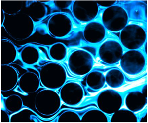
Figure 1. (a) Schematics of the set-up. (b) Detail of a typical sectional view of the porous medium. The grains are coloured in grey. The white dots are passive fluorescent tracers seeding the fluid. (c) Overlay of successive images illustrating the fluid flow.

Figure 2. (a) Detail of a typical raw 2-D velocity field obtained by particle tracking. (b) Same field after post-processing. (c) Corresponding distributions of the 2-D velocity magnitude,  $U_{2\text{-}\text{D}}\equiv \sqrt{u^{2}+v^{2}}$.
The experimental set-up is sketched in figure 1(a). The porous medium consists of a 3-D random stack of rigid, spherical, poly(methyl methacrylate) (PMMA) grains (Engineering Laboratories Inc.) of diameter  $d=2~\text{mm}$. The grains are tightly packed in a long transparent container (
 $100d\times 12d\times 12d$). The fluid is forced through the porous medium with a constant flow rate using a translating stage (M-403.4 PD, not shown in the schematics) and a syringe placed at the top of the set-up. The fluid is collected at the bottom in a flexible container.
2.1 Porous medium, liquid and tracers
The PMMA grains composing the porous medium have been specifically chosen for their smooth surface, good transparency and monodispersity. The solid volume fraction is close to the random packing fraction of frictional spheres  $\simeq 0.58$ and the porosity (void fraction) is therefore
  $\simeq 0.42$. The fluid employed, Triton X-100, is Newtonian and has a large viscosity,
  $\unicode[STIX]{x1D702}=0.270~\text{Pa}~\text{s}$. The typical average fluid velocity is
  $\langle U\rangle \sim 100~\unicode[STIX]{x03BC}\text{m}~\text{s}^{-1}$. This yields a Reynolds number
  $\unicode[STIX]{x1D70C}\langle U\rangle d/\unicode[STIX]{x1D702}\sim 10^{-3}$, ensuring that inertial effects are negligible. At room temperature, the fluid refractive index (
 $\simeq 1.492$) is close to that of the PMMA grains (
 $\simeq 1.491$), which makes the porous medium nearly transparent. To optimize the transparency, we finely match both indices of refraction down to the fourth digit (Souzy et al. Reference Souzy, Lhuissier, Villermaux and Metzger2017) by adjusting the temperature of the water bath surrounding the porous medium to
  $T=28.1\pm 0.5\,^{\circ }\text{C}$. The flow visualizations and the dispersion experiments have been performed by seeding the fluid with small fluorescent particles (PMMA B-particles from MF-Rhodamine) as shown in figure 1(b). The particles have a diameter
  $d_{t}=3.23~\unicode[STIX]{x03BC}\text{m}$, which is much smaller than the pore size (
 $d_{t}\simeq d/620$). This allows an unprecedented resolution for passively sampling the fluid flow – as a comparison
  $d_{t}/d$ was around
  $1/63$,
  $1/32$ and
  $1/35$ for the measurements by Moroni & Cushman (Reference Moroni and Cushman2001), Datta et al. (Reference Datta, Chiang, Ramakrishnan and Weitz2013) and Carrel et al. (Reference Carrel, Morales, Dentz, Derlon, Morgenroth and Holzner2018), respectively. The particle diffusivity is negligible (the Péclet number based on their size,
  $\unicode[STIX]{x1D702}\langle U\rangle dd_{t}/k_{B}T$, where
  $k_{B}$ is the Boltzmann constant, is larger than
  $10^{10}$).
2.2 Imaging
The solid structure and fluid velocity inside the porous medium are imaged in a two-dimensional (2-D) plane formed by a planar vertical laser sheet, which is displaced across the porous medium to reconstruct the 3-D fields (see figure 1a). Each section of the porous medium illuminated by the sheet is imaged with a high-resolution camera (ORCA-Flash4.0,  $2048\times 1048~\text{pixels}$, 16 bit) mounted with a macroscopic lens (Sigma APO-Macro-180mm-F3.5-DG). This camera has been chosen for its linear response and its high signal-to-noise ratio. The laser sheet is formed by reflecting a laser beam (2 W, 532 nm) on a rotating mirror (
 ${\sim}10^{4}~\text{r.p.m.}$), which yields a highly uniform sheet. It is focused down to a thickness of
  ${\approx}60~\unicode[STIX]{x03BC}\text{m}$ using plano-convex lenses. Finally, scattered light is discarded with the help of a high-pass filter (590 nm) located before the lens; this ensures that only the light emitted by the fluorescent tracers is collected by the camera.
3 Three-dimensional velocity field
3.1 Velocity measurements
Figure 1(b) shows a zoom on a typical image where the grain sections are highlighted in grey. All the grains have the same size. The apparent size differences only arise from their different distances to the laser sheet plane. The fluid velocity is measured by tracking the fluorescent tracers (bright dots in the image) using the open-source particle tracking velocimetry software TracTrac developed by Heyman (Reference Heyman2019). The volume fraction of tracers is sufficiently small ( ${\sim}10^{-5}$) not to affect the flow. The algorithm tracks each individual tracer and provides its displacement between successive frames. Within this stationary flow, the velocity field is obtained by accumulating data over 1000 successive images (separated by 0.1 s) such that, in each pixel within the fluid, approximately 10 particles were detected and tracked. The strength of the present TracTrac algorithm is to provide the fluid velocity within each pixel (here the pixel size is
  $d/228$), thus largely outperforming any particle image velocimetry techniques in terms of spatial resolution. Figure 2(a) shows a map of the raw 2-D velocity amplitude
  $U_{2\text{-}\text{D}}/\langle U_{2\text{-}\text{D}}\rangle$, with
  $U_{2\text{-}\text{D}}\equiv \sqrt{u^{2}+v^{2}}$, obtained with the algorithm. The raw data are post-processed to successively (i) mask regions inside the grains, (ii) fill the few pixels where no tracer has been detected with the surrounding pixels’ median value, and (iii) smooth the velocity field using a Gaussian filter of width 5 pixels. The post-processed field is shown in figure 2(b). As shown in figure 2(c), the post-processing has a negligible effect on the velocity distribution.

Figure 3. (a) Experimental 3-D velocity field and microstructure. The colour scale encodes the fluid velocity magnitude,  $U=\sqrt{u^{2}+v^{2}+w^{2}}$. (b,c) Distributions of the velocity components (b)
  $u$ along the mean flow direction (
 $\boldsymbol{e}_{\boldsymbol{x}}$) and (c)
  $v,w$ along the transverse directions (
 $\boldsymbol{e}_{\boldsymbol{y}},\boldsymbol{e}_{\boldsymbol{z}}$). (d) Distribution of the velocity magnitude.
The 3-D velocity field is obtained by repeating the above 2-D velocity field measurement over two perpendicular sets of 50 vertical sections spaced by  $d/10$, as depicted in figure 1(a). The sampled volume of porous medium is
  $9d\times 5d\times 5d$. The two sets of 2-D fields are linearly interpolated to provide the three velocity components (
 $u,v,w$) in the three directions (
 $\boldsymbol{e}_{\boldsymbol{x}},\boldsymbol{e}_{\boldsymbol{y}},\boldsymbol{e}_{\boldsymbol{z}}$) over the whole sampled domain (
 $2048\times 1048\times 1048$ voxels). Finally, a weighted divergence correction scheme (Wang et al. Reference Wang, Gao, Wei, Li and Wang2017) is used to ensure that the interpolated field is divergence-free. Again, both the interpolation and the divergence-free algorithm have been checked to have a negligible effect on the velocity distributions.
The reconstructed 3-D velocity field is shown together with the porous medium microstructure in figure 3(a). It provides the three velocity components with a higher spatial resolution ( $d/228$) than the most recent numerical simulations performed at the pore scale (Maier et al. Reference Maier, Kroll, Kutsovsky, Davis and Bernard1998; Kang et al. Reference Kang, Anna, Nunes, Bijeljic, Blunt and Juanes2014; Jin et al. Reference Jin, Langston, Pavlovskaya, Hall and Rigby2016).
3.2 Velocity distributions
The distribution of the velocity components ( $u,v,w$) and magnitude
  $U=\sqrt{u^{2}+v^{2}+w^{2}}$ are presented in figure 3(b–d). The velocity distributions are similar to those reported from previous experiments (Datta et al. Reference Datta, Chiang, Ramakrishnan and Weitz2013; Holzner et al. Reference Holzner, Morales, Willmann and Dentz2015; Carrel et al. Reference Carrel, Morales, Dentz, Derlon, Morgenroth and Holzner2018) and numerical simulations (Dentz et al. Reference Dentz, Icardi and Hidalgo2018). The distribution of the streamwise component (
 $u$) is skewed towards positive values and has an exponential tail. Small negative velocities, indicating the presence of back-flow, are present, although with a very weak probability. The distributions of the transverse velocities (
 $v,w$) are symmetric and have exponential shapes. Last, the distribution of the velocity magnitude is also exponentially tailed but it is found to follow, at low velocity, a power law,
  $\text{p.d.f.}~(U)\propto U^{\unicode[STIX]{x1D6FC}}$, with a positive exponent,
  $\unicode[STIX]{x1D6FC}\simeq 0.89$. As discussed in the introduction, the characteristics of the velocity distribution at small velocities control the longitudinal dispersion behaviour (Berkowitz & Scher Reference Berkowitz and Scher1995; Bijeljic, Mostaghimi & Blunt Reference Bijeljic, Mostaghimi and Blunt2011). In order to clarify these crucial characteristics, we have refined the velocity measurements using a dynamic-range technique.
3.3 Refined measurements at low velocities
The tracking algorithm accurately detects the particle displacements from 0.1 to 5 pixels only. Below 0.1 pixel, the displacement signal compares with the noise level, and above 5 pixels, the algorithm is likely to swap neighbouring particles. This experimental limitation actually biases the velocity field, especially at low velocity. To circumvent this problem, a dynamic-range measurement is used. It consists in performing three measurements of the velocity field with a constant frame rate (as described in § 3.1) but with a 10-fold increase of the flow rate between each measurement. Note that this dynamic range measurement was performed only over a single vertical plane since the statistics of the fluid velocity over that plane is found to be identical and thus representative of that obtained over the whole sampled volume. For each measurement, only the velocities corresponding to particle displacements in the confidence range of 0.5–5 pixels are retained.

Figure 4. Dynamic-range velocity measurements. (a) Map showing the regions of the three ranges of measurement: (i) yellow, fastest regions of the flow measured at low flow rate; (ii) light blue, intermediate regions; (iii) dark blue, slowest regions measured at large flow rate. (b) Comparison between the velocity distributions obtained with the dynamic-range technique and with a single measurement (same data as in figure 2c).

Figure 5. (a) Distribution of the streamline orientation  $\cos \unicode[STIX]{x1D703}$ and average velocity magnitude for a given orientation
  $\langle U\rangle _{\cos \unicode[STIX]{x1D703}}$. Here
  $A$ and
  $B$ are normalizing constants (
 $A=a/\!\sinh a$,
  $B=2(a+b)\sinh a\sinh b/[ab\sinh (a+b)]$). Inset: definition of the streamline orientation
  $\unicode[STIX]{x1D703}$. (b) Relative distribution of the velocity magnitude for a given orientation. The black line represents (3.2). Inset: joint distribution of the magnitude and orientation.
Figure 4(a) shows the regions corresponding to the three velocity ranges of measurement, with the fastest regions of the flow (measured with the slowest flow rate) in yellow, the intermediate regions in light blue and the slowest regions (largest flow rate) in dark blue. The unbiased distribution of the 2-D velocity magnitude obtained with this dynamic-range technique is found to be flat at low velocity ( $\text{p.d.f.}(U_{2\text{-}\text{D}})\propto {U_{2\text{-}\text{D}}}^{0}$); see figure 4(b). This refined measurement procedure was not extended to the 3-D velocity field because of time constraints. However, since both
  $\text{p.d.f.}(u)$ and
  $\text{p.d.f.}(v)$ are flat at low velocity (see appendix A), the fact that
  $\text{p.d.f.}(U_{2\text{-}\text{D}}\equiv \sqrt{u^{2}+v^{2}})$ is also flat indicates that
  $u$ and
  $v$ are strongly correlated for small velocities (small values of
  $v$ are found where
  $u$ is small). Moreover, by symmetry,
  $w$ must be similarly correlated to
  $u$. Therefore, since the three velocity components are correlated and since their distribution is flat at low velocity, the 3-D velocity magnitude distribution,
  $\text{p.d.f.}(U_{3\text{-}D}\equiv \sqrt{u^{2}+v^{2}+w^{2}})$, must be flat as well at low velocity, in agreement with the numerical simulations performed recently by AlAdwani (Reference AlAdwani2017) and Dentz et al. (Reference Dentz, Icardi and Hidalgo2018).
Before discussing the implications of the shape of the velocity distribution on the dispersion process (see next section), we provide below an empirical correlation between the magnitude of the velocity and its orientation.
3.4 Velocity magnitude and orientation
Figure 5 presents the statistics of the streamline local orientations  $\text{p.d.f.}(\cos \unicode[STIX]{x1D703})$ and the mean velocity magnitude for a given orientation
  $\langle U\rangle _{\cos \unicode[STIX]{x1D703}}$ obtained from the 3-D experimental field over the velocity range for which measurements are accurate (
 $U\geqslant 0.3\langle U\rangle$). The streamline orientation is found to be well fitted by
  $\text{p.d.f.}(\cos \unicode[STIX]{x1D703})\propto \text{e}^{a\cos \unicode[STIX]{x1D703}}$, with a strong dependence on
  $\cos \unicode[STIX]{x1D703}$ embedded in the value of
  $a\simeq 4$; see inset of figure 5(a). This trend simply reflects that streamlines are strongly aligned with the longitudinal direction (
 $\boldsymbol{e}_{\boldsymbol{x}}$). Besides, we find that the magnitude of the velocity is also strongly correlated with its orientation. The average velocity magnitude for a given orientation
  $\langle U\rangle _{\cos \unicode[STIX]{x1D703}}$ increases when streamlines are more aligned with the flow, following the exponential trend
  $\langle U\rangle _{\cos \unicode[STIX]{x1D703}}\propto \text{e}^{b\cos \unicode[STIX]{x1D703}}$, with
  $b\simeq 1.5$.
These two experimental observations suggest a compact, 3-D characterization of the one-point statistics of the velocity field. Assuming for simplicity that the relative distribution of the velocity for each orientation is independent of the orientation (which is presumably a reasonable ansatz given the isotropy of the medium structure) imposes that the joint distribution of  $U$ and
  $\unicode[STIX]{x1D703}$ follows
 $$\begin{eqnarray}\text{p.d.f.}(U,\cos \unicode[STIX]{x1D703})=\frac{1}{\langle U\rangle _{\cos \unicode[STIX]{x1D703}}}\,\text{p.d.f.}(\cos \unicode[STIX]{x1D703})\,\text{p.d.f.}(U/\langle U\rangle _{\cos \unicode[STIX]{x1D703}}),\end{eqnarray}$$
where, as shown in figure 5(b), the relative velocity distribution is found experimentally to be close to
 $$\begin{eqnarray}\text{p.d.f.}(U/\langle U\rangle _{\cos \unicode[STIX]{x1D703}})=\text{e}^{-U/\langle U\rangle _{\cos \unicode[STIX]{x1D703}}}.\end{eqnarray}$$
 Equation (3.1) summarizes all the one-point information about the 3-D velocity field. It captures the main dependences observed experimentally, including an accurate description of the statistics at small velocity, since it embeds  $\text{p.d.f.}(U)\propto U^{0}$ for
  $U\ll \langle U\rangle _{\cos \unicode[STIX]{x1D703}}$.
4 Anomalous dispersion?
4.1 Dispersion measurements

Figure 6. Dispersion measurements: successive experimental images of a blob of small non-diffusive tracers flowing through the index-matched 3-D bead-pack (see also supplementary movie 1, available at https://doi.org/10.1017/jfm.2020.113). Only those particles contained in the  $z=0$ plane are visible (the field of view is
  $20d$ long in the streamwise direction and the tracers have a diameter
  $d_{t}=d/620$).

Figure 7. Dispersion measurements: trajectories of non-diffusive point particles advected numerically in the 3-D experimental velocity field (see also supplementary movies 2 and 3 for an immersive exploration of the 3-D velocity field (Pore Aventura 2019)). The six thick lines highlight six specific trajectories.
The dispersion process induced by this flow field is characterized in two ways: (i) directly, by monitoring the evolution of a blob of small non-diffusive particles (see figure 6), and (ii) indirectly, by numerically advecting non-diffusive point particles in the experimental 3-D velocity field (see figure 7).

Figure 8. Dispersion results. (a) Overlay of 13 blobs of non-diffusive tracers injected at 13 different locations in the porous medium at  $t/\unicode[STIX]{x1D70F}=0$ (red), 3 (green) and 10.5 (blue), with
  $\unicode[STIX]{x1D70F}=d/\langle U\rangle$. (b) Trajectories of 1250 non-diffusive point particles advected numerically in the experimental velocity field (grey) and their positions at
  $t/\unicode[STIX]{x1D70F}=0$ (red), 43 (green) and 136 (blue). (c) Variances of the position
  ${\unicode[STIX]{x1D70E}_{i}}^{2}\equiv \langle i^{2}\rangle -\langle i\rangle ^{2}$, with
  $i=x$,
  $y$ or
  $z$, obtained with both methods. The error bars represent the typical standard deviation between experimental runs. (d) Same data over a longer time.
The first method consists in injecting with a thin needle a small blob of fluid, typically of the size of the grains, seeded with non-diffusive fluorescent tracers (see § 2) in the bulk of the porous medium. Once the injection is completed, the flow is turned on and the evolution of the blob is captured within one plane illuminated by the laser sheet (see figure 6). The dispersion process is quantified through image processing by measuring the spatial variance  $\unicode[STIX]{x1D70E}^{2}$ of the tracer locations in both the longitudinal and transverse directions. The measurement can be achieved until
  $t/\unicode[STIX]{x1D70F}=10$, since all tracers have to remain in the field of view. The experiment is repeated 13 times by injecting the blob at different locations within the porous medium.
The second method consists in using the 3-D experimental fluid velocity field to advect numerically non-diffusive point particles. Some examples of trajectories are provided in figure 7. A total of 1250 tracers are positioned randomly within the fluid phase and advected using an explicit Runge–Kutta scheme. In order to allow a long-time advection ( $t/\unicode[STIX]{x1D70F}>100$), each point particle that reaches a boundary of the fluid domain is re-injected upwards at a location where the fluid velocity is the closest (in both magnitude and orientation) to its current velocity. This re-injection procedure was found to have no effect on the dispersion statistics. As shown in figure 3(d), the velocity distribution of these Lagrangian point particles is identical to that of the Eulerian velocity field, as expected in the present case of a volume-conserving flow (Dentz et al. Reference Dentz, Kang, Comolli, Le Borgne and Lester2016).
The dispersion results are gathered in figure 8. Figure 8(a) shows overlay images of the 13 blob experiments at  $t/\unicode[STIX]{x1D70F}=0$, 3 and 10.5, where
  $\unicode[STIX]{x1D70F}=d/\langle U\rangle$. The typical dispersion envelope explored by these non-diffusive particles is indicated with a dotted line. Figure 8(b) shows the trajectories of the 1250 numerical point particles (in grey) as well as their positions at
  $t/\unicode[STIX]{x1D70F}=0$, 43 and 136 (in colour). The dispersion process is quantified by measuring the variance of the tracers’ position, in both the longitudinal and transverse directions, i.e.
  ${\unicode[STIX]{x1D70E}_{i}}^{2}\equiv \langle i^{2}\rangle -\langle i\rangle ^{2}$, where
  $i$ stands for
  $x$,
$x$,  $y$ or
  $z$. The variances obtained with the two methods are compared in figure 8(c) until
  $t/\unicode[STIX]{x1D70F}=10$. After a short ballistic regime, where
  $\unicode[STIX]{x1D70E}^{2}\propto t^{2}$ for
  $t/\unicode[STIX]{x1D70F}\lesssim 1$, the variance becomes seemingly anomalous for
  $1\lesssim t/\unicode[STIX]{x1D70F}\leqslant 10$. It is super-diffusive in the streamwise direction (
 $\unicode[STIX]{x1D70E}_{x}^{2}\propto t^{1.4}$) and sub-diffusive transversely (
 ${\unicode[STIX]{x1D70E}_{y}}^{2}\propto t^{0.7}$). Note that similar exponents have also been reported for the same range of advection times by Kang et al. (Reference Kang, Anna, Nunes, Bijeljic, Blunt and Juanes2014), who simulated the fluid flow in the 3-D pore space of a real rock. Moreover, although the 3-D velocity field is slightly biased at small velocities (as discussed in § 3.3), the streamwise and transverse dispersions obtained from the numerical advection are very similar to those measured directly in the set-up, which validates the numerical advection procedure.
To characterize the dispersion over longer times, we rely on numerical advection measurements. These measurements, presented in figure 8(d), show that the anomalous trends are only transient. For  $t/\unicode[STIX]{x1D70F}\gtrsim 10$, both the longitudinal and transverse dispersions eventually relax to a Fickian regime with variances following
 $$\begin{eqnarray}\unicode[STIX]{x1D70E}_{x}^{2}=2D_{\Vert }t\quad \text{and}\quad {\unicode[STIX]{x1D70E}_{y}}^{2}={\unicode[STIX]{x1D70E}_{z}}^{2}=2D_{\bot }t,\end{eqnarray}$$
respectively, with dispersion coefficients equal to
 $$\begin{eqnarray}D_{\Vert }\simeq (0.45\pm 0.05)d^{2}/\unicode[STIX]{x1D70F}\quad \text{and}\quad D_{\bot }\simeq (0.027\pm 0.002)d^{2}/\unicode[STIX]{x1D70F}.\end{eqnarray}$$
4.2 Link between dispersion and velocity distributions
The above measurements require some interpretation. The ballistic dispersion regime lasts typically until  $t\sim \unicode[STIX]{x1D70F}$, which indicates that the velocity of the tracers remains correlated over a displacement of order
  $d$. Beyond that time, the dispersion becomes anomalous.
In the longitudinal direction, velocities are essentially positive and the (super-diffusive) anomaly is controlled by the occurrence of the smallest velocities, which significantly delay some of the tracers. Following Berkowitz et al. (Reference Berkowitz, Cortis, Dentz and Scher2006), we model the displacement of each tracer as a succession of random longitudinal steps with a fixed length  $d$ and a random velocity
  $u$ that is conserved over the step but uncorrelated with the previous velocities. This CTRW is fully constrained by the velocity distribution. It is computed numerically for
  $10^{4}$ uncorrelated tracers (the first step length is chosen randomly between 0 and
  $d$, to account for the random initial position of the tracers, and the tracers’ displacement is sampled with a substep scale at desired times). For an exponential velocity distribution, which has the same flat shape (
 $p(u)\propto u^{0}$) at low velocity and the same mean value
  $\langle u\rangle /\langle U\rangle =0.79$ as the experimental distribution, the CTRW yields
  $\unicode[STIX]{x1D70E}_{x}^{2}/d^{2}\sim \log (t/\unicode[STIX]{x1D70F})t/\unicode[STIX]{x1D70F}$. As shown in figure 9, this trend is in good agreement with the experimental data over the range
  $1\lesssim t/\unicode[STIX]{x1D70F}\lesssim 10$ and agrees with the prediction that the dispersion is super-diffusive when the low-velocity exponent of the distribution (
 $p(u)\propto u^{\unicode[STIX]{x1D6FC}}$) satisfies
  $\unicode[STIX]{x1D6FC}\leqslant 0$ (Berkowitz et al. Reference Berkowitz, Cortis, Dentz and Scher2006).
To understand the final relaxation towards a Fickian regime, the finite minimal velocity of the tracers has to be considered. Indeed, in a real flow, advected tracers always have a finite minimal velocity. This finite minimal velocity can arise from the finite size  $d_{t}$ of the tracers, which prevents them from sampling the smallest fluid velocities close to the walls. In the present case, this minimal velocity can be estimated as
  $U_{min}/\langle U\rangle \approx 10d_{t}/d\approx 0.02$, since the typical pore size is equal to
  $d/10$; see figure 3(a). The finite minimal velocity can also result from the finite thermal diffusivity of the tracers. Such tracers can escape from a region of low velocity more quickly through the effect of molecular diffusion than through the effect of advection alone (Saffman Reference Saffman1959). In such a case, the minimal velocity is
  $U_{min}\sim (10\langle U\rangle /d)\times \unicode[STIX]{x1D6FF}$, where
  $\unicode[STIX]{x1D6FF}\sim \sqrt{Dd/U_{min}}$ is the transverse diffusive displacement and
  $D$ is the tracers’ (thermal) diffusion coefficient. This yields
  $U_{min}/\langle U\rangle \approx (10^{2}D/\langle U\rangle d)^{1/3}$. This minimal velocity has a crucial impact on the longitudinal dispersion, precisely because the dispersion anomaly is controlled by the low velocities. To illustrate this point, we simulate a CTRW based on the same exponential distribution but discarding all velocities below
  $U_{min}$. As shown in figure 9, when
  $U_{min}/\langle U\rangle$ is set to 0.01, 0.03, 0.1 or 0.2, the variance relaxes to a Fickian regime beyond
  $t_{F}/\unicode[STIX]{x1D70F}\simeq 100$, 33, 10 and 5, respectively, instead of following
  $\log (t/\unicode[STIX]{x1D70F})t/\unicode[STIX]{x1D70F}$ as previously. The Fickian regime is reached once the velocities of all the tracers become decorrelated. The CTRW dispersion matching the experiments is obtained with
  $U_{min}/\langle U\rangle =0.1$. This is consistent with the fact that the 3-D velocity distribution, as a result of the limited experimental resolution, departs from a flat distribution below
  $U/\langle U\rangle \simeq 0.1$ (see figure 3d).

Figure 9. Streamwise and transverse variances,  $\unicode[STIX]{x1D70E}_{x}^{2}/d^{2}$ and
  ${\unicode[STIX]{x1D70E}_{z}}^{2}/d^{2}$, obtained from the numerical advection in the 3-D experimental velocity field compared to the CTRW simulations. CTRW based on a flat velocity distribution (
 $\text{p.d.f.}(u)\propto u^{0}$ at small
  $u$) yields a persistent anomalous dispersion
  $\unicode[STIX]{x1D70E}_{x}^{2}/d^{2}\sim \log (t/\unicode[STIX]{x1D70F})t/\unicode[STIX]{x1D70F}$ (green line), which matches the experiments until
  $t/\unicode[STIX]{x1D70F}\sim 10$. For a flat distribution truncated below
  $U_{min}/\langle U\rangle =0.01$, 0.03, 0.1 and 0.2, the dispersion eventually becomes Fickian (
 $\unicode[STIX]{x1D70E}_{x}^{2}\propto t$) after
  $t_{F}/\unicode[STIX]{x1D70F}\approx 100$, 33, 10 and 5, respectively (grey lines). The experimental transverse dispersion is well captured by a CTRW with anticorrelated velocities (see text). The black dashed lines indicate the slope 1.
By contrast, the sub-diffusive anomaly in the transverse direction is not controlled by the smallest velocities but is a consequence of the meandering trajectories inside the porous medium, which makes the transverse velocities alternately positive and negative with similar magnitudes. This can be shown by simulating a unidimensional CTRW with a large probability  $p$ that the tracers change direction between steps. Using an exponential velocity distribution with a mean value
  $\langle v\rangle /\langle U\rangle =0.34$ identical to the experimental distribution (figure 3c) and setting
  $p=0.86$ results in a sub-diffusive dispersion in good agreement with the experiments. As shown in figure 9, the transient sub-diffusive trend is recovered over the typical duration
  $\unicode[STIX]{x1D70F}/(1-p)$, over which velocities remain anticorrelated.
With the above information at hand, we can explain the values of the dispersion coefficients ( $D_{\Vert }$ and
  $D_{\bot }$) obtained in the (long-time) Fickian regime. For tracers with a constant velocity over the porous scale
  $d$, the duration of each step is
  $\unicode[STIX]{x1D70F}^{\prime }=d/U$. The probability of
  $\unicode[STIX]{x1D70F}^{\prime }$ is fully constrained by the tracer velocity distribution
  $p_{U}(U)$ according to
  $p_{\unicode[STIX]{x1D70F}^{\prime }}(\unicode[STIX]{x1D70F}^{\prime })=(d^{2}/\langle U\rangle \unicode[STIX]{x1D70F}^{\prime 3})p_{U}(d/\unicode[STIX]{x1D70F}^{\prime })$, which is defined over
  $0\leqslant \unicode[STIX]{x1D70F}^{\prime }\leqslant d/U_{min}$ (see details in appendix B). Now, the probability that a tracer has moved over a large curvilinear distance
  $s$, i.e. that
  $s/d$ steps have been covered at a given time
  $t$, is given by the
  $s/d$-fold convolute of
  $p_{\unicode[STIX]{x1D70F}^{\prime }}$, i.e.
  ${p_{\unicode[STIX]{x1D70F}^{\prime }}}^{\ast \,s/d}(t)$. Using the central limit theorem and
  $\langle x\rangle /s=\langle u\rangle /\langle U\rangle$, the streamwise spatial variance
  $\unicode[STIX]{x1D70E}_{x}^{2}$ can be expressed in terms of the variance of the step durations,
  ${\unicode[STIX]{x1D70E}_{\unicode[STIX]{x1D70F}^{\prime }}}^{2}\equiv \langle \unicode[STIX]{x1D70F}^{\prime 2}\rangle -\langle \unicode[STIX]{x1D70F}^{\prime }\rangle ^{2}$, as
  $\unicode[STIX]{x1D70E}_{x}^{2}/d^{2}\approx \langle u\rangle ^{2}/\langle U\rangle ^{2}{\unicode[STIX]{x1D70E}_{\unicode[STIX]{x1D70F}^{\prime }}}^{2}t/\unicode[STIX]{x1D70F}^{3}$. For a flat velocity distribution (
 $p_{U}(U)\propto U^{0}$), the step duration variance is prescribed by the minimal velocity as
  ${\unicode[STIX]{x1D70E}_{\unicode[STIX]{x1D70F}^{\prime }}}^{2}/\unicode[STIX]{x1D70F}^{2}\approx \ln (\langle U\rangle /U_{min})$. Altogether, one obtains
 $$\begin{eqnarray}D_{\Vert }=\frac{\unicode[STIX]{x1D70E}_{x}^{2}}{2t}\approx \frac{1}{2}\ln \left(\frac{\langle U\rangle }{U_{min}}\right)\frac{\langle u\rangle ^{2}}{\langle U\rangle ^{2}}\frac{d^{2}}{\unicode[STIX]{x1D70F}},\end{eqnarray}$$
 which makes precise how the dispersion coefficient depends on the minimal velocity  $U_{min}$. With the experimental values
  $\langle u\rangle \simeq 0.79\langle U\rangle$ and
  $U_{min}\simeq 0.1\langle U\rangle$, equation (4.3) yields
  $D_{\Vert }\simeq 0.7d^{2}/\unicode[STIX]{x1D70F}$, which is within the same order of magnitude as the measured value
  $0.45d^{2}/\unicode[STIX]{x1D70F}$ reported in (4.2).
In the transverse direction, the same arguments together with the probability,  $1-p$, that a step is not anticorrelated with the previous ones, give similarly
 $$\begin{eqnarray}D_{\bot }=\frac{{\unicode[STIX]{x1D70E}_{y}}^{2}}{2t}=\frac{{\unicode[STIX]{x1D70E}_{z}}^{2}}{2t}\approx \frac{1}{2}\ln \left(\frac{\langle U\rangle }{U_{min}}\right)(1-p)\frac{\langle v\rangle ^{2}}{\langle U\rangle ^{2}}\frac{d^{2}}{\unicode[STIX]{x1D70F}}.\end{eqnarray}$$
 For the experimental values  $\langle v\rangle =\langle w\rangle \simeq 0.34\langle U\rangle$ and
  $U_{min}\simeq 0.1\langle U\rangle$, this yields
  $D_{\bot }\simeq 0.02d^{2}/\unicode[STIX]{x1D70F}$, which is also found to be close to the measurement
  $0.027d^{2}/\unicode[STIX]{x1D70F}$ reported in (4.2).
5 Stretching laws
We now turn to the key information required to model mixing, namely, the statistics of the stretching of the fluid material lines.
5.1 Method
The stretching distributions are determined by advecting numerically material lines in the experimental velocity field. We follow the same procedure as in Souzy et al. (Reference Souzy, Lhuissier, Villermaux and Metzger2017), initially developed by Meunier & Villermaux (Reference Meunier and Villermaux2010), but adapted here to a 3-D velocity field. The material lines consist of segments joining non-diffusive tracers initially separated by a distance  $l_{0}=d/120$. Each tracer is advected individually, but every time the length of a segment is doubled, the segment is split in two by adding a new tracer in the middle. The mean stretching rate, averaged over many segments, is found to be independent of the integration error. Moreover, by using different smoothing procedures, we checked that the residual noise arising from measurement artefacts and from the interpolation of the velocity field does not affect the value of the mean stretching rate. For instance, applying an additional smoothing procedure after the interpolation of the velocity field reduced the mean residual velocity divergence by 20 % but had no consequence on the value of the mean stretching rate, which remains constant within 1 %.

Figure 10. (a) Evolution of a material line advected numerically in the 3-D experimental velocity field (see also supplementary movie 4). The line is displayed at four successive times. (b) Projection of the line on the transverse plane ( $\boldsymbol{e}_{\boldsymbol{y}},\boldsymbol{e}_{\boldsymbol{z}}$) at the same times. (c) Mean and variance of the logarithm of the elongation versus time (
 $\unicode[STIX]{x1D70E}_{ln\,\unicode[STIX]{x1D70C}}^{2}\equiv \langle \ln \unicode[STIX]{x1D70C}^{2}\rangle -\langle \ln \unicode[STIX]{x1D70C}\rangle ^{2}$). (d) Distribution of the logarithm of the elongation at four successive times. The black lines show the Gaussian distributions having the same mean and variance as the experimental ones.
When advecting segments, we used the same re-injection procedure as for the dispersion measurements but applied to the segment centre. Again, we checked that this re-injection has no effect on the stretching statistics. The statistics of elongations are renormalized to account for the fact that the most elongated segments become more numerous in time. This procedure allows us to resolve the small-scale stretching and folding of the line at all times. An example of the evolution of a material line is shown in figure 10 (see also supplementary movie 5). As the line is advected across the pores, it stretches and folds with patterns reminiscent of chaotic advection. We consider the local elongation of the line
 $$\begin{eqnarray}\unicode[STIX]{x1D70C}(t)\equiv \frac{l(t)}{l_{0}},\end{eqnarray}$$
 where  $l(t)$ is the current line length between initially adjacent tracers.
5.2 Results
Figure 10(b,c) shows the experimental stretching laws obtained from the statistics of 6000 initial segments advected for a duration  $t/\unicode[STIX]{x1D70F}\approx 20$ (no initial transient is observed because the tracers have been pre-advected for
  $t=5\unicode[STIX]{x1D70F}$ to obtain a steady-state distribution of segment orientation). We find that both the mean logarithm of the elongation,
  $\langle \ln \unicode[STIX]{x1D70C}\rangle$, and its variance,
  $\unicode[STIX]{x1D70E}_{ln\,\unicode[STIX]{x1D70C}}^{2}\equiv \langle (\ln \unicode[STIX]{x1D70C})^{2}\rangle -\langle \ln \unicode[STIX]{x1D70C}\rangle ^{2}$, grow linearly in time and with almost identical slopes, according to
 $$\begin{eqnarray}\langle \ln \unicode[STIX]{x1D70C}\rangle =\unicode[STIX]{x1D706}t/\unicode[STIX]{x1D70F}\quad \text{and}\quad \unicode[STIX]{x1D70E}_{ln\,\unicode[STIX]{x1D70C}}^{2}=\unicode[STIX]{x1D707}t/\unicode[STIX]{x1D70F},\end{eqnarray}$$
 with  $\unicode[STIX]{x1D706}\simeq \unicode[STIX]{x1D707}\simeq 0.47\pm 0.03$.
Moreover, as shown in figure 10(c), the distribution of the elongation logarithm is well captured by the Gaussian distribution
 $$\begin{eqnarray}\text{p.d.f.}(x=\ln \unicode[STIX]{x1D70C})=\frac{1}{\sqrt{2\unicode[STIX]{x03C0}}\unicode[STIX]{x1D70E}_{ln\,\unicode[STIX]{x1D70C}}}\exp \left[-\frac{(x-\langle \ln \unicode[STIX]{x1D70C}\rangle )^{2}}{2\unicode[STIX]{x1D70E}_{ln\,\unicode[STIX]{x1D70C}}^{2}}\right].\end{eqnarray}$$
 The distribution of elongation is thus log-normal and its two first moments, i.e. the mean elongation,  $\langle \unicode[STIX]{x1D70C}\rangle$, and the variance,
  ${\unicode[STIX]{x1D70E}_{\unicode[STIX]{x1D70C}}}^{2}$, follow
 $$\begin{eqnarray}\langle \unicode[STIX]{x1D70C}\rangle =\text{e}^{(\unicode[STIX]{x1D706}+\unicode[STIX]{x1D707}/2)t/\unicode[STIX]{x1D70F}}\simeq \text{e}^{(3/2)\unicode[STIX]{x1D706}t/\unicode[STIX]{x1D70F}}\quad \text{and}\quad {\unicode[STIX]{x1D70E}_{\unicode[STIX]{x1D70C}}}^{2}=\text{e}^{2(\unicode[STIX]{x1D706}+\unicode[STIX]{x1D707})t/\unicode[STIX]{x1D70F}}\simeq \text{e}^{4\unicode[STIX]{x1D706}t/\unicode[STIX]{x1D70F}}.\end{eqnarray}$$
 The exponential stretching revealed by the above advection procedure is reminiscent of Lagrangian chaos. The intensity of such chaotic dynamics is usually characterized by the Lyapunov exponent  $\unicode[STIX]{x1D706}$, which quantifies the average long-term growth rate of infinitesimal fluid element lengths. In our case, the Lyapunov exponent is simply the average steady-state stretching rate of the line,
 $$\begin{eqnarray}\unicode[STIX]{x1D706}\equiv \unicode[STIX]{x1D70F}\langle \dot{\unicode[STIX]{x1D70C}}/\unicode[STIX]{x1D70C}\rangle _{t\gg \unicode[STIX]{x1D70F}}.\end{eqnarray}$$
 Figure 11(a) shows the evolution of  $\unicode[STIX]{x1D70F}\langle \dot{\unicode[STIX]{x1D70C}}/\unicode[STIX]{x1D70C}\rangle _{t\gg \unicode[STIX]{x1D70F}}$ as a function of time when no pre-advection has been performed. The orientation of the segments is random at
  $t/\unicode[STIX]{x1D70F}=0$. As expected from fluid incompressibility, the mean stretching rate is equal to zero initially; see inset of figure 11(a). Then, over of a few strain units, the segments orient with the flow and
  $\unicode[STIX]{x1D70F}\langle \dot{\unicode[STIX]{x1D70C}}/\unicode[STIX]{x1D70C}\rangle$ converges to its steady-state value
  $\unicode[STIX]{x1D706}\simeq 0.47$.

Figure 11. (a) Mean stretching rate versus time. Inset: same data in semi-logarithmic scales. The dashed line shows the Lyapunov exponent (long-time value)  $\unicode[STIX]{x1D706}\simeq 0.47\pm 0.03$. The error bar reflects the time fluctuations of the Lyapunov exponent once steady state is reached. (b) Mean projected stretching rates along
  $\boldsymbol{e}_{\boldsymbol{x}}$,
  $\boldsymbol{e}_{\boldsymbol{y}}$ and
  $\boldsymbol{e}_{\boldsymbol{z}}$ versus time, where
  $\boldsymbol{e}_{\boldsymbol{l}}\equiv \boldsymbol{l}/|\boldsymbol{l}|$ is the line tangent direction.
We also estimate the anisotropy of the material line stretching by computing the mean components of the stretching rate  $\langle \dot{\unicode[STIX]{x1D70C}}/\unicode[STIX]{x1D70C}|\boldsymbol{e}_{\boldsymbol{l}}\boldsymbol{\cdot }\boldsymbol{e}_{\boldsymbol{x}}|\rangle$,
  $\langle \dot{\unicode[STIX]{x1D70C}}/\unicode[STIX]{x1D70C}|\boldsymbol{e}_{\boldsymbol{l}}\boldsymbol{\cdot }\boldsymbol{e}_{\boldsymbol{y}}|\rangle$ and
  $\langle \dot{\unicode[STIX]{x1D70C}}/\unicode[STIX]{x1D70C}|\boldsymbol{e}_{\boldsymbol{l}}\boldsymbol{\cdot }\boldsymbol{e}_{\boldsymbol{z}}|\rangle$, where
  $\boldsymbol{e}_{\boldsymbol{l}}\equiv \boldsymbol{l}/|\boldsymbol{l}|$ is the line tangent direction. Note that this definition does not include the effect of the line rotation; thus it only quantifies the line stretching. These stretching rates are thus different from the growth rate of the projected elongations. As shown in figure 11(b), each component follows a similar evolution, with an initial transient and a relaxation towards a positive steady-state value. Interestingly, we find that the mean stretching rate parallel to the flow,
  $\langle \dot{\unicode[STIX]{x1D70C}}/\unicode[STIX]{x1D70C}|\boldsymbol{e}_{\boldsymbol{l}}\boldsymbol{\cdot }\boldsymbol{e}_{\boldsymbol{x}}|\rangle$, is only 20 % larger than those measured in the transverse directions. This shows that, despite the symmetry breaking imposed by the mean flow, the random bead-pack structure of the porous medium induces strong fluctuations, which yield a close-to-isotropic stretching of fluid material lines.
6 Conclusion and discussions
Using advanced index-matching and particle-tracking techniques, we measured the pore-scale velocity in 3-D porous media at an unprecedented resolution. This allowed us to characterize in particular the low tail of the velocity p.d.f., which is critical for anomalous dispersion, and the distribution of local velocity gradients that control stretching and mixing. The three velocity components have been measured over a sample volume of  $9d\times 5d\times 5d$ with a resolution of
  $d/228$. This extensive set of data, which may be used as a benchmark for numerical simulations, has been made available online (Souzy et al. Reference Souzy, Lhuissier, Meheust, Le Borgne and Metzger2018), as well as the purposely developed 3-D velocity field explorer software Pore Aventura (Pore Aventura 2019).
Particular attention has been paid to the statistics of small velocities, which control the anomalous longitudinal dispersion trend frequently reported in porous media. Dynamic-range velocity measurements, increasing the accuracy at low velocity, have allowed us to show experimentally that the distribution of the velocity magnitude is flat at low velocity ( $\text{p.d.f.}(U)\propto U^{0}$), in agreement with recent numerical results (AlAdwani Reference AlAdwani2017; Dentz et al. Reference Dentz, Icardi and Hidalgo2018).
The dispersion process has been investigated with non-diffusive tracers by three methods: (i) experiments with blobs of small particles; (ii) numerical advection on the experimental 3-D velocity field; and (iii) continuous-time random walk (CTRW) simulations. These investigations have shown that the dispersion process is transiently anomalous ( $\unicode[STIX]{x1D70E}_{x}^{2}/d^{2}\sim \ln (t/\unicode[STIX]{x1D70F})t/\unicode[STIX]{x1D70F}$ and
  ${\unicode[STIX]{x1D70E}_{y,z}}^{2}/d^{2}\lesssim t/\unicode[STIX]{x1D70F}$) until a time scale
  $t_{F}\approx d/U_{min}$ set by the low-end cutoff
  $U_{min}$ of the tracer velocity distribution, before it eventually becomes Fickian (
 $D_{\Vert }\simeq 0.45d^{2}/\unicode[STIX]{x1D70F}$ and
  $D_{\bot }\simeq 0.027d^{2}/\unicode[STIX]{x1D70F}$) beyond
  $t_{F}$. This low-velocity cutoff is always present owing to the finite size of the tracers (
 $U_{min}/\langle U\rangle \approx 10d_{t}/d$) or to their finite diffusivity (
 $U_{min}/\langle U\rangle \approx (10^{2}D/\langle U\rangle d)^{1/3}$). It also determines the value of the long-time longitudinal dispersion coefficient (
 $D_{\Vert }\propto \ln (\langle U\rangle /U_{min})d^{2}/\unicode[STIX]{x1D70F}$).
Finally, we provide the first experimental characterization of the full stretching statistics in a 3-D porous medium. The mean elongation of fluid material lines is found to grow exponentially in time ( $\langle \dot{\unicode[STIX]{x1D70C}}/\unicode[STIX]{x1D70C}\rangle \equiv \unicode[STIX]{x1D706}/\unicode[STIX]{x1D70F}$). This exponential trend is in sharp contrast to the linear growth reported from 2-D simulations and 2-D experiments performed at the pore scale (De Anna et al. Reference De Anna, Dentz, Tartakovsky and Le Borgne2014; Jiménez-Martínez et al. Reference Jiménez-Martínez, Le Borgne, Tabuteau and Méheust2017), or the power-law trends obtained for 2-D simulations at the Darcy scale (Le Borgne, Dentz & Villermaux Reference Le Borgne, Dentz and Villermaux2013; Le Borgne et al. Reference Le Borgne, Dentz and Villermaux2015), where the 2-D nature of these steady flows precludes the development of chaotic advection. Our experimental results thus confirm the chaotic nature of advection within 3-D porous media anticipated by Shaqfeh & Koch (Reference Shaqfeh and Koch1992) and Lester et al. (Reference Lester, Dentz and Le Borgne2016).
The Lyapunov exponent value  $\unicode[STIX]{x1D706}\simeq 0.47$ measured here is larger than those reported in numerical studies. Lester et al. (Reference Lester, Dentz and Le Borgne2016) obtained
  $\unicode[STIX]{x1D706}\simeq 0.1178$ for a model of random open network and Turuban et al. (Reference Turuban, Lester, Le Borgne and Méheust2018) found
  $\unicode[STIX]{x1D706}\simeq 0.073$ for a crystalline sphere pack. These differences could stem from the specific model of random open network considered and from the crystalline nature of the sphere pack, which presumably induces less stretching than the random packing investigated here. This point remains to be understood.
Last, measurements of the full statistics of elongations revealed that the long-time distribution of elongations is log-normal. This suggests an underlying multiplicative stretching process where, at small scales, material lines undergo multiplicative and uncorrelated stretching cycles having a finite persistence time. This paradigm has been reported previously for other complex flows, such as a random sine flow (Meunier & Villermaux Reference Meunier and Villermaux2010) or the flow within a sheared suspension of non-Brownian particles (Souzy et al. Reference Souzy, Lhuissier, Villermaux and Metzger2017), and appears to be generic to a large class of complex flows.
The above results provide a solid basis for a full description of mixing within a porous medium. By characterizing the flow kinematics, the laws of dispersion and stretching provided here enable predictions for the evolution of the concentration distribution of a diffusive scalar (Villermaux Reference Villermaux2019). They also appeal for further experimental work to obtain quantitative measurements of the evolution of the concentration distribution (e.g. using the techniques developed by Souzy et al. (Reference Souzy, Zaier, Lhuissier, Le Borgne and Metzger2018)). Finally, it is worth recalling that these kinematic laws were obtained in a random pack of monodisperse spheres, that is to say, in an isotropic porous medium with a narrow pore size distribution. Whether they could serve as a kinematic framework for predicting mixing processes in real porous media encountered in geophysics, such as soils composed of sand or rocks, would be an interesting subject to address in future studies.
Acknowledgements
We warmly thank C. Wang for making his weighted divergence correction scheme available, J. Heyman for doing so with his particle tracking algorithm, and D. Lester, R. Turuban, E. Villermaux and P. Meunier for fruitful discussions. We also thank S. Noel for machining the experimental set-up, and N. Barret and L. Forner for developing Pore Aventura, a dedicated 3-D velocity field explorer software. This work has been supported by ANR ScienceFriction, by Labex MEC ANR-10-LABX-0092, by ANR-11-IDEX-0001-02 and by ERC consolidator grant ReactiveFronts 648377.
Declaration of interests
The authors report no conflict of interest.
Supplementary movies
Supplementary movies are available at https://doi.org/10.1017/jfm.2020.113.
Appendix A. Refined distributions of the velocity components
Figure 12 shows that the velocity distributions of both components  $u$ and
  $v$, obtained with the dynamic-range measurement technique, are flat at low velocities.

Figure 12. Distribution of the velocity components  $u$ and
  $v$ and of the 2-D velocity magnitude
  $U_{2\text{-}\text{D}}=\sqrt{u^{2}+v^{2}}$ obtained from the dynamic-range velocity measurement.
Appendix B. Dispersion coefficients in the Fickian regime
We derive the expressions for the dispersion coefficients  $D_{\Vert }$ and
  $D_{\bot }$ in the (long-time) Fickian regime for the CTRW considered in § 4.2, i.e. by modelling the displacement of tracers as a succession of random steps with a fixed length
  $d$ and a random velocity
  $U$ that is conserved over the step but uncorrelated with the previous velocities. In this framework, the probability for the duration,
  $\unicode[STIX]{x1D70F}^{\prime }=d/U$, of each step is fully constrained by the tracer velocity distribution. Indeed, the probability
  $p_{\unicode[STIX]{x1D70F}^{\prime }}(\unicode[STIX]{x1D70F}^{\prime })$ is directly related to the velocity distribution sampled per step (i.e. sampled per unit of length rather than per unit of time)
  $p_{U|step}$ according to
 $$\begin{eqnarray}p_{\unicode[STIX]{x1D70F}^{\prime }}(\unicode[STIX]{x1D70F}^{\prime })=\left|\frac{\unicode[STIX]{x2202}U}{\unicode[STIX]{x2202}\unicode[STIX]{x1D70F}^{\prime }}\right|p_{U|step}(U)=\frac{d}{\unicode[STIX]{x1D70F}^{\prime 2}}\,p_{U|step}\left(\frac{d}{\unicode[STIX]{x1D70F}^{\prime }}\right).\end{eqnarray}$$
 This distance-sampled velocity distribution is simply related to the Lagrangian (time-sampled) distribution  $p_{U}(U)$ that is actually measured, by
 $$\begin{eqnarray}p_{U|step}(U)=\frac{U}{\langle U\rangle }p_{U}(U).\end{eqnarray}$$
Together with (B 1) this gives
 $$\begin{eqnarray}p_{\unicode[STIX]{x1D70F}^{\prime }}(\unicode[STIX]{x1D70F}^{\prime })=\frac{d^{2}}{\langle U\rangle \unicode[STIX]{x1D70F}^{\prime 3}}p_{U}\left(\frac{d}{\unicode[STIX]{x1D70F}^{\prime }}\right).\end{eqnarray}$$
 From the statistics of  $\unicode[STIX]{x1D70F}^{\prime }$, those for the total distance travelled by a tracer in the limit of a large number of steps can be obtained as follows. The probability that, at given time
  $t$, a tracer has displaced by a large curvilinear distance
  $s$, i.e. that it has made a large number
  $s/d$ of steps, is simply the
  $s/d$-fold convolute of
  $p_{\unicode[STIX]{x1D70F}^{\prime }}$, that is to say,
  ${p_{\unicode[STIX]{x1D70F}^{\prime }}}^{\ast \,s/d}(t)$. From the central limit theorem and under the present assumption of a Fickian dispersion, the spatial variance
  ${\unicode[STIX]{x1D70E}_{s}}^{2}\equiv \langle s^{2}\rangle -\langle s\rangle ^{2}$ can be expressed in terms of the variance of the step durations,
  ${\unicode[STIX]{x1D70E}_{\unicode[STIX]{x1D70F}^{\prime }}}^{2}\equiv \langle \unicode[STIX]{x1D70F}^{\prime 2}\rangle -\langle \unicode[STIX]{x1D70F}^{\prime }\rangle ^{2}$, according to
 $$\begin{eqnarray}\frac{{\unicode[STIX]{x1D70E}_{s}}^{2}}{d^{2}}\approx \frac{{\unicode[STIX]{x1D70E}_{\unicode[STIX]{x1D70F}^{\prime }}}^{2}}{\unicode[STIX]{x1D70F}^{2}}\frac{t}{\unicode[STIX]{x1D70F}}.\end{eqnarray}$$
 In the long-time limit one has both  $\langle x\rangle /s=\langle u\rangle /\langle U\rangle$ and
  $\langle x^{2}\rangle /s^{2}=\langle u\rangle ^{2}/\langle U\rangle ^{2}$. Therefore, the streamwise variance follows
 $$\begin{eqnarray}\frac{\unicode[STIX]{x1D70E}_{x}^{2}}{d^{2}}\approx \frac{\langle u\rangle ^{2}}{\langle U\rangle ^{2}}\frac{{\unicode[STIX]{x1D70E}_{\unicode[STIX]{x1D70F}^{\prime }}}^{2}}{\unicode[STIX]{x1D70F}^{2}}\frac{t}{\unicode[STIX]{x1D70F}}.\end{eqnarray}$$
Last, by definition of the variance of the step duration, one has
 $$\begin{eqnarray}\frac{{\unicode[STIX]{x1D70E}_{\unicode[STIX]{x1D70F}^{\prime }}}^{2}}{\unicode[STIX]{x1D70F}^{2}}\equiv \int _{0}^{d/U_{min}}\frac{\langle U\rangle }{\unicode[STIX]{x1D70F}^{\prime }}p_{U}\left(\frac{d}{\unicode[STIX]{x1D70F}^{\prime }}\right)\text{d}\unicode[STIX]{x1D70F}^{\prime }-\left(\int _{0}^{d/U_{min}}\frac{\langle U\rangle }{\unicode[STIX]{x1D70F}^{\prime 2}}p_{U}\left(\frac{d}{\unicode[STIX]{x1D70F}^{\prime }}\right)\text{d}\unicode[STIX]{x1D70F}^{\prime }\right)^{\!2},\end{eqnarray}$$
 which embeds the anomalous dispersion condition: for a vanishing minimal velocity ( $U_{min}=0$), the variances
  $\unicode[STIX]{x1D70E}_{\unicode[STIX]{x1D70F}^{\prime }}^{2}$ and
  $\unicode[STIX]{x1D70E}_{x}^{2}$ are finite only if the low-velocity exponent of the Lagrangian velocity distribution is positive (
 $p_{U}(U)\propto U^{\unicode[STIX]{x1D6FC}}$ with
  $\unicode[STIX]{x1D6FC}>0$). For a finite
  $U_{min}$ and a flat velocity distribution (
 $p_{U}(U)\propto U^{0}$), the dependence to
  $U_{min}$ follows
 $$\begin{eqnarray}\frac{{\unicode[STIX]{x1D70E}_{\unicode[STIX]{x1D70F}^{\prime }}}^{2}}{\unicode[STIX]{x1D70F}^{2}}\approx \ln \left(\frac{\langle U\rangle }{U_{min}}\right).\end{eqnarray}$$
Making use of (B 5) and (B 7), one recovers the expression provided in (4.3):
 $$\begin{eqnarray}D_{\Vert }=\frac{\unicode[STIX]{x1D70E}_{x}^{2}}{2t}\approx \frac{1}{2}\ln \left(\frac{\langle U\rangle }{U_{min}}\right)\frac{\langle u\rangle ^{2}}{\langle U\rangle ^{2}}\frac{d^{2}}{\unicode[STIX]{x1D70F}},\end{eqnarray}$$
 which specifies how the dispersion coefficient depends on the minimal velocity  $U_{min}$.
In the transverse direction, the same arguments apply if one realizes that among  $n$ pairs of steps, only the
  $(1-p)n$ pairs for which the two steps have the same direction contribute to the dispersion. The variance is thus decreased by the same factor
  $(1-p)$, and replacing
  $\langle u\rangle$ by
  $\langle v\rangle$ in (B 8) yields the expression provided in (4.4):
 $$\begin{eqnarray}D_{\bot }=\frac{{\unicode[STIX]{x1D70E}_{y}}^{2}}{2t}=\frac{{\unicode[STIX]{x1D70E}_{z}}^{2}}{2t}\approx \frac{1}{2}\ln \left(\frac{\langle U\rangle }{U_{min}}\right)(1-p)\frac{\langle v\rangle ^{2}}{\langle U\rangle ^{2}}\frac{d^{2}}{\unicode[STIX]{x1D70F}}.\end{eqnarray}$$


