


1. Introduction
The interaction of turbulence with shock waves is of significant importance to the engineering community, particularly with respect to aerospace applications. Shock-turbulence interactions (STI) are prevalent in high-speed aerodynamics. Specifically, STI is a leading contributor to the challenges in hypersonic vehicle design because of its ability to significantly alter the fluid dynamics downstream through amplification of turbulent modes and modification of energy transport. Even in typical wind tunnel testing, the interaction of free-stream noise with inherent shock structures adds uncertainty and complexity to high-speed diagnostics. Due to the nonlinearity and coupling of modal interactions in the process, STI, even in its most basic form, is a complex problem.
Although it has been studied for several decades, the behaviour of STI is still largely uncertain. Modern direct numerical simulation (DNS) studies (Donzis Reference Donzis2012a; Larsson, Bermejo-Moreno & Lele Reference Larsson, Bermejo-Moreno and Lele2013) have brought into question classical STI theories based on the linear interaction analyses (LIA) of Ribner (Reference Ribner1954, Reference Ribner1955). These differences become increasing noticeable as the Mach number is increased beyond 2. At present, experimental data are not available to guide theory and reconcile these differences. This is especially true for non-intrusive measurements at high Mach number.
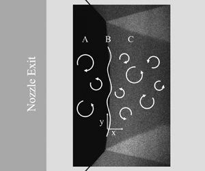
The overarching objective of this study was to provide detailed experimental measurements to quantify the role of a normal shock wave on the modification of turbulence through measurement of vortical and entropic fluctuations across a normal shock wave in a high Mach number wind tunnel environment. An experimental campaign took place within the Texas A&M University National Aerothermochemistry and Hypersonics Laboratory, in a pulsed wind tunnel facility. The target Mach number was selected to be sufficiently high to resolve the differences between classical (Ribner Reference Ribner1954, Reference Ribner1955), and contemporary theories (Larsson Reference Larsson2010; Donzis Reference Donzis2012a,Reference Donzisb) and simulations (Larsson et al. Reference Larsson, Bermejo-Moreno and Lele2013; Chen & Donzis Reference Chen and Donzis2019), while not introducing undue experimental difficulty (e.g. the excessive heating to avoid liquefaction at hypersonic conditions). Hence, Mach 4.5 was targeted. Generating controlled turbulence at high Mach number represents a significant technical challenge. However, vortical (velocity), entropy (temperature) and acoustic (pressure) disturbances are commonly observed in high-speed wind tunnel free streams. These small-scale free-stream disturbances are typically assumed to be uncorrelated in a linearized approach (Kovasznay Reference Kovasznay1953). Thus, the wind tunnel free stream was selected as the test bed for these experiments. A Mach-stem generator was selected to produce a normal shock within the wind tunnel free stream. An open-wedge design was developed to enable optical access. An image of the Mach stem at Mach 4.5 is shown in figure 1 with a diagram outlining the interests of the study.

Figure 1. Schematic of canonical shock–turbulence interaction in relation to example Mach 4.5 Mach-stem flow. (A) Free-stream turbulent flow; (B) example wrinkling of normal shock due to STI; (C) downstream amplified turbulent flow; (W) Mach-stem generator ‘wedges’ illustrating the experiment configuration in the tunnel (not to scale), black lines shown connecting to the Mach-stem image represent the leading edge oblique shock waves.
The instruments were selected to be non-intrusive and responsive to the rapid jump in properties across a shock wave, which occur over a spatial range corresponding to approximately 3–5 molecular mean free paths. High energy, pulsed (10 Hz), laser-based systems to monitor the velocity and temperature of seeded nitric oxide were available. Hence, molecular tagging velocimetry (MTV) and two-line planar laser induced fluorescence (PLIF) instrumentation was selected to quantify the vortical and entropic fluctuations. The expected uncertainties in the velocity and temperature were less than 0.5 %, which was sufficient to characterize the expected changes across the normal shock. The free-stream gas was selected to be nitrogen to improve the PLIF signal-to-noise ratio over that of air, where the presence of oxygen leads to significant quenching of nitric oxide fluorescence.
A new pulsed wind tunnel was developed to achieve large data sets ( $>$10 000 samples). The pulsed facility was synchronized to the laser systems with a duty cycle of nominally 20 seconds. However, the overall test duration was unbounded within the available infrastructure. The facility repeatability was within 3 % and 4 % for velocity and temperature, respectively, which was sufficient to quantify the expected changes across the normal shock. Optical measurement of the acoustic (sound) fluctuations was not attempted in this study due to the unavailability of instrumentation. This is not considered a strong drawback as Quadros, Sinha & Larsson (Reference Quadros, Sinha and Larsson2016b) has shown good agreement between LIA and DNS for the acoustic field.
2. Literature review
Lists of current computational and experimental works in canonical shock turbulence interaction are given in tables 1 and 2 respectively. Classical investigations of STI typically take the LIA approach first attributed to Ribner (Reference Ribner1954, Reference Ribner1955, Reference Ribner1987) and Moore (Reference Moore1953). While such a linearized approach will inherently lose some turbulence information, its use has been widely accepted, particularly in the cases of strong shock waves and weak turbulence where the assumptions most closely match the environment. Attempts have also been made to apply rapid distortion theory to the shock problem (Lele Reference Lele1992; Jacquin, Cambon & Blin Reference Jacquin, Cambon and Blin1993b); however, the results indicated this approach was insufficient in predicting STI behaviour. With the rise of modern computation abilities, contemporary works have mainly transitioned to large eddy simulation (LES) and DNS approaches. These modern approaches have observed divergence from classic LIA solutions, particularly as Mach numbers of interest have increased. It has been shown (Rotman Reference Rotman1991; Ryu & Livescu Reference Ryu and Livescu2014), however, that for small turbulent Mach number  $(M_t)$ DNS solutions converge to LIA. Lee, Lele & Moin (Reference Lee, Lele and Moin1993) observed that increasing
  $M_t$ leads to a discrepancy in turbulent kinetic energy (TKE) enhancement, which may account for some of the disagreement between these approaches. Donzis (Reference Donzis2012a) introduced a scaling parameter ‘
 $K$’ as the ratio of laminar shock thickness to Kolmogorov length scale, which allowed for easy categorization of STI. It was believed that some of the disparity between differing studies was a result of incomplete comparison, influencing variables typically left out in previous works, the turbulent Mach number and Taylor Reynolds number (
 $M_t$,
  $Re_\lambda$), were captured in the value of ‘
 $K$’ for a more clear indication of behaviour. More recently, Chen & Donzis (Reference Chen and Donzis2019) continued the exploration of similarity scaling, and was able to collapse all available data of amplification factors, including simulations that stray from classic LIA assumptions. Another factor in simulations, separating experimental and computational results, is likely the influence of upstream correlations between Kovasznay modes. Few works have explored these influences, namely Hannappel, Hauser & Friedrich (Reference Hannappel, Hauser and Friedrich1995); Mahesh, Lele & Moin (Reference Mahesh, Lele and Moin1997) and Jamme et al. (Reference Jamme, Cazalbou, Torres and Chassaing2002). Mahesh et al. (Reference Mahesh, Lele and Moin1997) suggested that negative correlation between upstream velocity and temperature fluctuations would increase amplification of TKE as well as vortical and thermodynamic fluctuations across the shock wave. This observation is thought to be of particular importance in the current study.
Table 1. Computational works in canonical STI.

Table 2. Current experimental works in canonical STI. P is pressure; T is temperature; ρ is density, and U is velocity.

The majority of experimental works in canonical STI have been studied in shock tube facilities, observing decaying turbulent fields interacting with traveling shock waves. Measurements are typically made with the use of hot-wires and pressure transducers and the authors report significant amplification of turbulent intensities as well as length and time scales (Trolier & Duffy Reference Trolier and Duffy1985; Honkan & Andreopoulos Reference Honkan and Andreopoulos1990, Reference Honkan and Andreopoulos1992; Honkan, Watkins & Andreopoulos Reference Honkan, Watkins and Andreopoulos1994; Briassulis & Andreopoulos Reference Briassulis and Andreopoulos1996; Xanthos, Briassulis & Andreopoulos Reference Xanthos, Briassulis and Andreopoulos2002; Agui, Briassulis & Andreopoulos Reference Agui, Briassulis and Andreopoulos2005). These results have shown moderate agreement with theory, although some limitations exist in these comparisons due to the experimental conditions and unknowns. Shadowgraphy, schlieren and speckle photography (Haas & Sturtevant Reference Haas and Sturtevant1987; Hesselink & Sturtevant Reference Hesselink and Sturtevant1988; Keller & Merzkirch Reference Keller and Merzkirch1994) have been performed as well, though the results are rather limited and high errors have been reported.
A few studies have been performed observing STI for a stationary shock wave using the laser Doppler velocimetry (LDV) technique in conventional wind tunnel facilities (Jacquin, Blin & Geffroy Reference Jacquin, Blin and Geffroy1993a; Barre, Alem & Bonnet Reference Barre, Alem and Bonnet1996). It was determined in both cases, however, that the LDV was unable to fully capture the turbulent motion and thus was not sufficient for STI investigation. Another wind tunnel investigation of STI in a large-scale blowdown facility measured total pressure fluctuations and turbulent length scales for a Mach 6 stationary shock wave, the highest experimental Mach number investigated thus far in canonical STI (Mai & Bowersox Reference Mai and Bowersox2014). The authors believe the current work is the first truly non-intrusive investigation of velocity and temperature fluctuations in canonical STI, at one of the highest experimental Mach numbers in the field to date.
3. Facility
All experiments in this work were conducted in the pulsed hypersonic adjustable contour expansion nozzle for aero-thermochemical test environments (PHACENATE) facility located at the National Aerothermochemistry and Hypersonics Laboratory (NAL) at Texas A&M University in College Station, Texas. The PHACENATE (pronounced ‘fascinate’) facility nominally operates with a 60 ms total run time with 10–15 ms of stable flow and a duty cycle of 10–20 s. The pulsed operation is ideal for laser diagnostic based experiments, and allows for large-sample data collection in order to analyse fluctuating quantities.
PHACENATE is a tabletop-scale facility with a converging–diverging planar nozzle (exit dimensions  $10.2\ \textrm {cm}\times 10.2\ \textrm {cm}$) that exits into a rectangular test section (dimensions
  $25.4\ \textrm {cm}\ \textrm {H}\times 25.4\ \textrm {cm}\ \textrm {D}\times 58.4\ \textrm {cm}\ \textrm {L}$). The nozzle was designed using a method of characteristics approach, similar to the method described in Semper, Pruski & Bowersox (Reference Semper, Pruski and Bowersox2012). The facility supports a variable Mach number range by allowing the height of the nozzle throat to be adjusted via a series of shims while the two nozzle planes are allowed to rotate in order to maintain a constant exit area.
The test section has a series of mounting holes on the upper and lower walls of the cell for instrumentation capabilities. A series of rails was mounted to these holes, which were used to support a set of aerodynamic wedges with one degree of freedom. The test section provides optical access from all sides with 15.2 cm diameter schlieren quality windows in both sidewalls for imaging and  $17.8\ \textrm {cm}\ \textrm {L}\times 2.5\ \textrm {cm}\ \textrm {W}$ fused silica windows in the upper and lower walls for laser access. There are multiple window ports on the top and bottom walls of the tunnel allowing adjustment of diagnostic location. Several window blanks were outfitted as well, to allow additional pressure ports or sting assemblies to be used in the facility.
To achieve hypersonic conditions, a set of vacuum pumps evacuate both the test cell and nozzle to 133 Pa (0.5 Torr) and the settling chamber is pressurized between 170 and 650 kPa. The facility is operated on a high pressure liquid nitrogen (N $_{2}$) tank running through a regulator to the supply line. A set of mass flow controllers are located in line to allow controlled mixing of nitric oxide (NO) into the supply for optical diagnostic capabilities. The gas mixture enters a pebble bed heater which acts to pre-heat the supply and force mixing for even composition. The temperature of the heater is set such that the expansion process of the gas entering the tunnel and flowing through the nozzle will not result in liquefaction. The heated gas exits the pebble bed and fills a 0.1 m
 $^3$ reservoir which enters the settling chamber through a pair of 2.5 cm poppet valves, pictured in figure 2. The poppet valves operate with energize times of 12 ms and are actuated by a series of MHJ Festo valves.

Figure 2. Image of the PHACENATE facility. Included labels are the mass flow controllers (A), pebble bed heater (B), inlet tank (C), poppet valves (D) and knife gate (E) leading to the dump tank and vacuum pumps through the wall.
A Quantum Composer 9520 series pulse delay generator is used to control tunnel operation. The Festo valves are triggered to open and close the poppet valves and then the lasers, cameras and data acquisition are triggered at optimal time delays. The pulse delay generator has picosecond resolution on 8 channels with  $<$50 ps jitter, and thus, is capable of controlling both tunnel operation and laser timing simultaneously. A custom program, written in LabVeiw, integrates tunnel control with data acquisition and system monitoring under a single graphical user interface.
4. Wind tunnel model
The goal for the wind tunnel model used in this work was to produce a ‘canonical STI’ flow field by forming a freestanding normal shock wave in an optically accessible location. This was achieved by creating a Mach stem at the nozzle exit, through a set of opposing aerodynamic wedges (Hornung & Robinson Reference Hornung and Robinson1982; Mouton & Hornung Reference Mouton and Hornung2007). Predictions of Mach-stem height and growth rates are detailed in Mouton & Hornung (Reference Mouton and Hornung2007). The flow geometry is a function of incoming Mach number, specific heat ratio and deflection surface geometry. From the work of Mouton and Hornung, only the angle and length of the leading edge of the deflection model is needed to satisfy the geometry unknowns. In an experimental work by Chpoun & Leclerc (Reference Chpoun and Leclerc1999), it is shown that Mach-stem formation and height is consistent between different model geometries, so long as the leading edge angle and length are kept constant. From this, Mach-stem generator models can be developed for specific incoming flow conditions.
The model design in this work was chosen by optimizing the leading edge angle and overall wedge height (easily related to leading edge length) using a Matlab procedure developed by Mai & Bowersox (Reference Mai and Bowersox2014) following the routine of Mouton & Hornung (Reference Mouton and Hornung2007). For an expected Mach number range of 4 to 6, the ideal leading edge angle was found to be 32 $^{\circ }$. This was determined by looking at the critical deflection angles for both the incident and reflected shocks and selecting an angle that remains between the two curves for the entire Mach number range. An overall height of 0.953 cm was chosen to optimize the Mach-stem height within the bounds of tunnel blockage allowance and the expected core flow diameter of 5.1 cm.
An additional consideration for the model design was optical access to the near region of the Mach stem from multiple directions. Camera access from the side of the tunnel was needed for imaging, as well as access for multiple laser sheets from the top or bottom of the tunnel. For this purpose, the model was designed with an open body concept where the leading edge is followed by an acute return angle creating a triangular profile, in contrast to a typical hypersonic body design. It was believed that the absence of a model structure downstream of the triple point may also help to stabilize the flow by removing the shock–boundary layer interaction of the reflected shock. Finally, the wedge implemented a swept back design to delay the influence of the shear layer of the nozzle sidewalls in hopes of minimizing blockage and stabilizing the flow. Figure 3 shows a schematic of the model on its rail assembly as it would be installed in the tunnel, as well as a cut-out view that shows the leading edge profile.

Figure 3. Schematic and cut-out view of final wedge design.
5. Experimental methods and data reduction
5.1. Total pressure measurements
Total pressure measurements were conducted using a constructed Pitot pressure probe. A Kulite XCEL-100-5A pressure sensor was flush mounted in precision stainless steel tubing. Three sections of increasing diameter tubing were connected downstream of the sensor head with epoxy-smoothed transitions to bring the outer diameter from the size of the transducer (0.26 cm) up to 0.6 cm (further described in Mai (Reference Mai2014)). The Pitot probe could then be mounted in a sting assembly to position it in the test section. The Kulite sensor was sampled at 300 kHz and the signal was low pass filtered at 50 kHz before being recorded on the computer's data acquisition system.
Total pressure measurements were taken along the centreline of the nozzle exit plane in vertical and horizontal directions. Fifty runs were recorded at each of 9 locations across the nozzle exit plane while the probe was moved manually using a transition stage. Target locations of the probe were measured with a ruler across the nozzle exit and marked on the transition stage, accuracy of the location of the probe is of the order of 0.2 cm. For each location a 2 ms section of data was taken from each run in the region of stable pressure. The same 2 ms section of data from the settling chamber pressure was normalized against itself and used to correct the Pitot signal to account for shot-to-shot influences over time. This was done for both vertical and horizontal rakes.
5.2. Laser system description and experiment configuration
Two identical pulsed laser systems were used in this study for excitation of nitric oxide in various LIF techniques. Each system consisted of an injection seeded Spectra Physics PRO-290-10 Nd:YAG laser and a Sirah Cobra Stretch dye laser with a sum frequency mixing unit. The YAG laser operated at 10 Hz with a linewidth of 0.003 cm $^{-1}$, and was tuned for output in both second and third harmonics (532 nm and 355 nm respectively). A fundamental beam was generated in the dye laser by pumping a dye solution consisting of Rhodamine 610 and Rhodamine 640 in methanol with the first harmonic output of the YAG. The resulting fundamental beam was tuneable in the range of 600 to 630 nm. The dye fundamental beam was then mixed with the third harmonic output from the YAG in a Sirah SFM-355 mixing unit, resulting in an ultraviolet (UV) 223 to 227 nm output beam. Typical linewidth and power of the UV beam was 0.08 cm
 $^{-1}$ and 5–12 mJ pulse
 $^{-1}$ respectively.
The experimental configuration used for both laser based methods is depicted in figure 4. The model wedges were installed flush with the exit plane of the nozzle and spaced 5.1 cm apart vertically. The optimal vertical spacing for the wedges was determined via schlieren imaging flow visualization, where the Mach stem's height was maximized while remaining downstream of the wedge geometry. A Pitot pressure probe was mounted outside of the laser diagnostic area, in the lower corner of the core flow, to monitor tunnel conditions. A Princeton Instruments PI-MAX4 ICCD camera was mounted for viewing from the right-hand side of the tunnel.

Figure 4. Model wedge configuration for MTV and PLIF thermometry experiments. (a) Image of actual configuration in tunnel; (b) diagram showing model wedge and Pitot probe position from behind, looking straight into nozzle exit.
The tunnel N $_{2}$ supply was pre-seeded with 0.5 %–1.0 % NO and pre-heated to achieve 375 K in the tunnel settling chamber. The initial laser was timed at 30–32 ms following initial tunnel valve opening and the second laser followed at a 1.7
  $\mathrm {\mu }$s time delay. This time delay was selected to minimize the uncertainty in the velocimetry technique, and was used in both laser based methods for consistency. The camera was liquid cooled to
  $-$35 C with the intensifier enabled. The dual image feature setting was used and camera gates were set to 3/100 ns for the velocimetry ‘write’/‘read’ exposures and 10–15 ns for both PLIF exposures.
5.3. Molecular tagging velocimetry
Velocity measurements were made across a normal shock using a single component MTV approach. Two lasers were used in the MTV technique, one ‘write’ laser to initially excite the ground state NO, and one ‘read’ laser that would later target the tagged  $v''=1$ NO, as previously demonstrated in Sánchez-González, Bowersox & North (Reference Sánchez-González, Bowersox and North2014). The final turning mirrors and sheeting optics for both lasers were mounted to an optical breadboard, which in turn was mounted to a linear transition stage on a rail system. A diagram of this set-up is shown in figure 5. The linear transition stage was used to optimize the location of the ‘write’ laser lines in relation to the normal shock wave during operation of the tunnel. The camera gate was set to 100 ns exposure so that signal from the scattered laser between the focused lines could be detected in order to reveal the shock location. The transition stage was then adjusted until the ‘write’ line was just downstream of the shock wave, usually with a separation of roughly 5 pixels. Once the lines were in optimal location, the transition stage was locked to prevent accidental motion.

Figure 5. Diagram of experiment set-up for MTV measurements.
For each Reynolds number condition a series of images was taken. First a dotcard image was taken to align and focus the camera on the laser excitation region, as well as provide a distance conversion factor to be used in post-processing. The background intensity was corrected by taking a ‘dark-charge’ image of the covered camera lens and subtracting this from each frame. In order to confirm the location of the shock wave in post-processing, a long term PLIF exposure of NO(0,0) was recorded and averaged over 100 frames. Finally, the MTV images were recorded at several locations. Five hundred image pairs were taken in the ‘optimal’ position described previously. The transition stage would then be adjusted to shift the laser lines 5–10 pixels farther downstream, and 500 image pairs were taken at the new location. This was repeated until 4 total locations had been recorded.
All velocimetry images in this study were processed using a custom program written in Matlab. Cross-correlation was performed using the built in ‘ $x$-corr’ Matlab function. First, each image pair was divided into ‘sub-images’ representing a region of single pixel height surrounding the location of the initial ‘write’ laser line. A threshold value was subtracted from each sub-image to remove the background signal and avoid corruption of the cross-correlation results. The ‘
 $x$-corr’ function was then applied and the resulting correlation matrix was cropped around the peak value and fitted with a third-order polynomial with centring and scaling applied.
A goodness of fit ( $r^2$) value was recorded for the correlation function so that the user could remove poor correlation results. An example cross-correlation result is shown in figure 6. It was found that the correlation fit would underestimate the correlation peak value in most cases with the polynomial fit. While the peak value itself is not meaningful, in order to make sure the location of the peak was as accurate as possible a secondary fitting procedure was applied. If the initial polynomial fit returned a goodness of fit value above a user specified threshold (typically 0.95), the application would crop even closer around the peak and perform another polynomial fit. Including more points initially allows for poor correlations, without strong peaks, to be excluded from further processing; and it was found to be within 0.5 pixels of the true peak. The secondary fitting further reduced this uncertainty to 0.1 pixels.

Figure 6. Cross-correlation example of a selected sub-image pair. The far (a) shows the normalized and thresholded sub-images, where the delayed image has been shifted by the correlation peak. In the (b) is the primary cross-correlation fit, and to the (c) is the secondary cross-correlation fit. Each is cropped around the peak value. A third order polynomial fit is applied with 95 % confidence bounds, and the resulting peak and goodness-of-fit  $r^2$ value are displayed at the top.
The recorded sub-pixel correlation peak was then converted to a velocity value via the pixel-to-metre conversion factor and time delay. This was repeated for all ‘sub-image’ regions across each image pair recorded in the series. The velocity and goodness of fit values were then sent to post-processing where mean and fluctuating values could be determined across the region of interest.
5.4. PLIF thermometry
Temperature measurements were made across a normal shock wave by a two-line PLIF thermometry technique, similar to that of Sánchez-González et al. (Reference Sánchez-González, Bowersox and North2014). The ‘read’ lasers in this study were tuned to probe transitions in the  $A^2\varSigma ^+(v'=0)- X^2\varPi (v''=0)$ band for ground state NO. For the nominal flow Mach number of 4.4, the expected mean temperature conditions were 77 K in the free stream and 361 K downstream of the normal shock wave. Target rotational states were chosen based on the Boltzmann population distributions of ground state NO at these temperatures. The rotational states
  $J''=1$ and
  $J''=8$ were chosen to maximize temperature sensitivity, particularly in the region downstream of the normal shock, while retaining reasonable signal potential from both regions of flow. Laser wavelengths were set for these rotational states and the power was balanced to
  $\sim$1.5 mJ pulse
 $^{-1}$ for both lasers.
A schematic of the experimental set-up for PLIF thermometry is shown in figure 7. Both lasers were introduced through the top window of the tunnel. In order to optimize the overlap of the laser sheets, the angle between the beams was minimized by mounting the final turning mirrors as close to each other as possible without clipping the beams. Both lasers were sent through a cylindrical lens to alter the circular profile into a planar sheet oriented in the direction of flow. A Princeton Instruments PI-MAX4 ICCD camera was mounted on the right-hand side of the tunnel for image collection.

Figure 7. Diagram of experimental set-up for PLIF thermometry.
A dotcard image was taken first, to focus the camera on the plane of the laser sheets. The background intensity was corrected in situ by subtracting a ‘dark-charge’ image of the covered camera lens from each frame. Five hundred image pairs were taken of the normal shock region for each Reynolds number condition and processed as described below. This was repeated in the same region of flow with the model wedges removed to further characterize the free-stream conditions. Additional image pairs were taken in regions of known temperature for calibration and image correction purposes during processing.
Thermometry images were processed using a custom application, written in Matlab. Free-stream images were initially processed following a conventional approach for linear LIF thermometry to establish baseline conditions. It was believed that the high laser intensity needed to obtain signal in the low density free stream led to a LIF response in the higher density post-shock region that was at the edge of the linear limit, possibly in the transitional to saturated regime for LIF thermometry. A separate processing routine was written to examine the Mach-stem PLIF images, where each region of the flow was individually analysed for an assumed mean temperature based on the previously established conditions. Because the quantities of interest in this study were fluctuations, and the mean flow conditions are well known conventionally, it was determined that this ‘in situ’ processing would be sufficient for the scope of this analysis.
In this two-line PLIF technique, temperature is determined via (5.1), where  $R_{12}$ is the ratio of LIF signals from rotational states ‘1’ and ‘2’,
  $C_{12}$ is a calibration constant based on experimental conditions,
  ${\rm \Delta} E$ is the energy separation between the states,
  $k$ is Boltzmann's constant and
  $T$ is the rotational temperature.
 \begin{equation} R_{12}=C_{12}\exp({-{\rm \Delta} E/kT}).\end{equation}
 The processing routine analysed the upstream and downstream locations as separate images. Calibration images were not used in this routine. Instead, a mean temperature was assumed based on the previous free-stream measurements and conventional shock-jump relations. The calibration constant ( $C_{12}$) was then specified to match this assumed temperature for the image intensity ratio (
 $R_{12}$) values at each pixel. This temperature specification method essentially acts as a laser profile correction step, combined with a temperature calibration, as is typically seen in the conventional approach. The raw images were cropped to view only the normal shock region with fluorescence signal, and then a region in front of and behind the normal shock was selected for further processing. Next, the images were binned in two dimensions for both pre- and post-shock regions, in this case a bin size of
  $4\times 4$ was selected to optimize both signal and resolution. The mean value of the pixels within each bin, excluding negative or ‘not a number’ values, was recorded and returned as the value for the entire bin.
Each pixel was then analysed individually to determine the appropriate  $C_{12}$ value and resulting mean and fluctuating temperatures. For each pixel coordinate,
  $R_{12}$ was first determined for all image pairs. Spurious
  $R$ values beyond three standard deviations from the mean
  $R$ value were removed for the determination of
  ${C_{12}}^{\prime }$. A
  ${C_{12}}^{\prime }$ value was then selected such that the resulting mean temperature, calculated for the range of
  $R$ values, would match the specified mean temperature of the region. This was done through manipulation of the standard PLIF thermometry equation into (5.2) to find ‘
 $\left \langle {{C_{12}}^{\prime }}\right \rangle$’ based on the given
  $R_{12}$ range and specified mean temperature.
 \begin{equation} \langle {{C_{12}}^{\prime}}\rangle=\langle {\exp({(\ln(R_{12})+{\rm \Delta} E/k\bar{T})})}\rangle . \end{equation}
 Once the appropriate  ${C_{12}}^{\prime }$ value was determined for a given pixel coordinate, temperature values for each image pair at that coordinate were calculated and recorded. This was repeated across both regions of interest, and the resulting temperature data were sent to post-processing. Mean and fluctuating temperatures were analysed for each region, the results of which are discussed in the next section.
6. Results
A list of the experiments performed in this work and the coinciding tunnel conditions is given in table 3. Total pressure measurements were taken during ‘free-stream’ studies only, while ‘Mach-stem’ investigations were purely optical investigations with wind tunnel models installed. The tunnel conditions remain comparable across the individual measurement campaigns, and the results between free-stream and pre-shock Mach-stem measurements show good agreement. During two of the Mach-stem investigations it was noted that a heater malfunction warning occurred. During these tests, the proportional-integral-derivative loop was reset during tunnel operation, and it was observed that the reservoir temperature increased above the desired temperature range by not more than 2 K for a period of several minutes (3–9 tunnel shots). Interrogation of the PLIF images for the course of these measurement campaigns showed no distinguishable indication of the isolated heater events, and the mean behaviour of the results again show good agreement with the measurements where no heater warnings occurred; thus it is believed that the effects were negligible.
Table 3. List of experiments and relevant tunnel conditions.

*Denotes a heater malfunction warning, the pebble bed heater PID loop was reset during tunnel operation and the supply temperature may have temporarily increased above the desired range. RMS, root mean square.
6.1. Total pressure characterization
Characterization of the free-stream total pressure was performed by traversing a Pitot pressure probe across the centreline of the nozzle exit taking snapshots of data. The total pressure was measured at nine locations across the vertical and horizontal nozzle exit centreline. Following the procedure previously described, a section of data was analysed for each location to determine the mean and fluctuating total pressure components across the nozzle exit plane. Plots of these are shown in figures 8 and 9 below. The uncertainty in the location of the probe at each point is of the order 0.2 cm. The model wedges, when installed, inhabit the area within  $\pm$0.5
  $x/l$ and
  $\pm$0.5
  $y/h$. Within this region, no significant anomalies in the mean or fluctuating total pressures are seen.

Figure 8. Total pressure traverse measurements for three Reynolds conditions in horizontal and vertical directions.

Figure 9. Total pressure fluctuation measurements for three Reynolds conditions in horizontal and vertical traverse directions.
Total pressure fluctuations were found to be  $\sim$2 % for all three cases. The
  $Re/m=2.1\times 10^6$ case was marginally lower. It is noted that it is expected that a significant portion (up to 50 %) of the fluctuating content was not resolved due to filtering and the physical size of the total pressure sensor. This would indicate an increase in the reported total pressure fluctuations by up to a factor of 2. However, the level of free-stream disturbances observed here are comparable to the results of Mai & Bowersox (Reference Mai and Bowersox2014) when their facility experienced turbulent boundary layers. Whereas the laminar boundary layer cases in their facility had significantly reduced free-stream disturbances. This comparison indicates that the present nozzle experienced turbulent boundary layers at all conditions.
The pressure and temperature data taken during each tunnel run were used in conjunction with isentropic and shock-jump relations to determine the expected bulk conditions for velocity and temperature in the Mach-stem flow. These values and their uncertainties are listed in table 4.
Table 4. Expected Mach-stem conditions.
6.2. MTV across normal shock
MTV experiments were performed on the Mach-stem flow at four locations downstream of the normal shock wave for each Reynolds condition. The measurement locations were determined in post-processing and were found to inhabit the region within 0.1 to 0.4 mm downstream of the normal shock wave. Early measurements taken further downstream showed signs of significant acceleration due to the convergence of the shear layer, thus the domain was restricted to the close region where this influence was minimized. The free-stream measurements were taken at a distance 1.6 to 2.0 mm upstream of the shock wave. Further, the centre 300 pixels were extracted for analysis to avoid potential interactions with the shear layer or influences of shock curvature. It was determined that the curvature led to a maximum change in shock angle of 2.5 $^{\circ }$ across the domain, which accounts for a maximum difference of 0.004 in the normal Mach number component. Given this analysis, it is believed the slight curvature had no measurable effect within the region. This final interrogation window is shown in figure 10, overlaid on a PLIF image of the Mach stem at
  $Re/m = 5.2\times 10^6$ for visual reference.

Figure 10. MTV measurement domain overlaid on PLIF image of Mach stem at  $Re/m = 5.2\times 10^6$.
The mean and fluctuating velocities across the shock wave for each of the Reynolds conditions is presented in table 5 below. The mean velocities are found to be within the uncertainty of the expected conditions. The uncertainty in cross-correlation peak estimation is believed to be of the order of 0.1 pixels following secondary fitting procedures, which does not account for the 3 % difference in mean velocities observed. It is believed the main source of variability in velocity determination arises from the uncertainty of actual tunnel conditions during typical operation. Higher free-stream and post-shock velocity fluctuations are noted in the lowest Reynolds condition, opposed to expectation. This trend is consistent with the free-stream measurements performed without model wedges installed, thus it is believed that the operation of the facility at such a low pressure leads to an increase in free-stream disturbances, possibly due to mass flow inconsistencies through the control valves at this condition.
Table 5. Mean and fluctuating velocities across a normal shock. Ranges shown for the four measurement locations of each Reynolds condition. The subscript FS denotes the upstream free-stream. The subscript DS denotes downstream of the normal shock-wave.

The mean velocities discussed above for the three Reynolds conditions were time-averaged over 500 samples. Figure 11 shows 10 randomly selected velocity profiles in comparison with the mean velocity for a single-line location in the middle Reynolds condition. This shows the overall spread of the data, and the result of the 500 sample averaging.

Figure 11. Several single-shot velocity profiles (colour) in comparison to the time-averaged mean velocity (black).
The number of data points (or image pairs) that were above the uncertainty cutoff of  $r^2=0.95$ across the measurement domain for each measurement location and Reynolds condition is listed in table 6. For the
  $Re/m = 2.1\times 10^6$ condition, the free stream shows 98 %–100 % of data points are retained using this cutoff. Downstream of the shock wave, however, there is an increase in the number of data points that are cutoff. The closest and farthest locations from the shock wave in the downstream case show the highest loss of data, at only 85 %–95 % retention. The discrepancy of the first location is possibly due to the proximity of the shock wave. In post-processing, the shock wave was found to alter the line shape at this first location in some of the image pairs (due to shot-to-shot inconsistency in shock formation). These images were excluded from further processing, however, it is possible that some inconsistency at this proximity was carried through in the remaining images as well. The low retention of the final location is presumably due to a discrepancy of laser intensity compared to the other cases. The
  $Re/m = 3.5\times 10^6$ condition experiences virtually no loss of data points to the uncertainty cutoff across the domain at all four measurement locations in both free stream and downstream of shock-wave measurements. Similarly, the highest Reynolds condition (
 $Re/m = 5.2\times 10^6$) experiences only minor data loss to the uncertainty cutoff, mostly occurring at the third measurement location downstream of the normal shock, although not at a level that produces concern.
Table 6. Per cent of data points above the uncertainty cutoff of  $r^2=0.95$ across the domain for each measurement location and Reynolds condition.

The velocity amplification factor is defined as the square of downstream fluctuations divided by upstream fluctuations,  $G={({U_{DS}}^\prime )}^2$/
  ${({U_{FS}}^\prime )}^2$, in this work. Amplification factor is plotted against distance downstream of the shock at each point in figures 12, 13 and 14 for the
  $Re/m = 2.1\times 10^6, 3.5\times 10^6$ and
  $5.2\times 10^6$ conditions respectively. All four measurement locations are included, and the mean value for each location is shown in black over the raw data. In the lowest Reynolds condition, the larger scatter observed closer to the shock is likely due, again, to the shock proximity and decrease in data retention. Moving farther downstream the amplification factor is found to trend towards unity with a spread of
  $\pm$0.2. Similar data point spread is observed in the
  $Re/m=3.5\times 10^6$ and
  $Re/m=5.2\times 10^6$ conditions, having mean values across the domain of 1.2 and 1.1 respectively.

Figure 12. Velocity amplification factor as a function of distance downstream of shock for  $Re/m=2.1\times 10^6$.

Figure 13. Velocity amplification factor as a function of distance downstream of shock for  $Re/m=3.5\times 10^6$.

Figure 14. Velocity amplification factor as a function of distance downstream of shock for  $Re/m=5.2\times 10^6$.
Average amplification factors of the three Reynolds conditions are plotted together in figure 15. There does not appear to be a significant Reynolds number trend in velocity amplification for these conditions. The low Reynolds condition is perhaps an anomaly, due to discrepancies described previously. The final two conditions lie in close proximity to each other, with perhaps a slight reduction in amplification with increasing Reynolds number.

Figure 15. Velocity amplification factors across shock for all Reynolds conditions.
Finally, the velocity amplification factors from this work are shown in relation to the LIA predictions from Donzis (Reference Donzis2012a) in figure 16. The mean values fall just below the LIA curve, with no distinct Reynolds number trend. Error bars representing the spread of the data in this study are found to almost reach the LIA prediction. In contrast, the other works included in Donzis’ study around this Mach number all lie well above the LIA prediction line. Although transverse velocity components were not measured in this work, an attempt can be made to estimate the TKE by assuming the post shock anisotropy is somewhere between 1 and 1.1 (Barre et al. Reference Barre, Alem and Bonnet1996; Larsson et al. Reference Larsson, Bermejo-Moreno and Lele2013). This would result in estimated amplification factors for TKE, ‘ $G_{TKE}$’, in the ranges 1.05–1.16, 1.18–1.30 and 1.10–1.21 for the Reynolds conditions
  $2.1\times 10^6\ {\rm m}^{-1}$,
  $3.5\times 10^6\ {\rm m}^{-1}$ and
  $5.2\times 10^6\ {\rm m}^{-1}$ respectively. In many cases,
  $G_{TKE}$ may be preferred for comparison (and may be considered a more fair comparison to LIA), thus this estimate is provided as a basis. However, due to the inability to measure the transverse velocity components, and for consistency with Donzis (Reference Donzis2012a) where G is defined as in this study, this work focuses on amplification of only the axial velocity in discussion.

Figure 16. Velocity amplification factors in relation to LIA predictions (adapted from Donzis (Reference Donzis2012a)).
6.3. Thermometry across normal shock
As previously discussed, the PLIF thermometry experiments were found to be outside of the linear regime. The mean temperature was specified for two defined regions in front of and behind the shock wave, based on the expected conditions determined previously. Each region was processed using averaged  $4\times 4$ pixel bins, and temperature outliers beyond three standard deviations from the mean were excluded. Using these techniques, there was at least 98 % retention of data points (image pairs) across the domain for all three Reynolds conditions. Contour plots of the fluctuating temperatures for each Reynolds condition are shown in figure 17. The two analysis regions are overlaid on the average PLIF image for each case for visual representation.

Figure 17. Temperature RMS fluctuations across shock for three Reynolds conditions. (a)  $Re/m =2.1\times 10^6$, (b)
  $Re/m = 3.5\times 10^6$, (c)
  $Re/m = 5.2\times 10^6$.
In thermometry processing, laser intensity fluctuations play into the systematic error of the results. It could be suggested that the observed fluctuations are truly a result of laser intensity and not turbulent properties. Figure 18 below shows the evolution of temperature fluctuations at 10 randomly selected pixels in each of the pre- and post-shock domains for the highest Reynolds condition. The scale is set to view only the first 200 image pairs to better visualize the correlation. It is expected that dominating laser intensity fluctuations would lead to correlated behaviour between all of the pixels, where true temperature fluctuations would be represented by 10 randomly fluctuating lines. While there are some common peaks, it can be seen that the 10 pixels act independently, therefore, it is believed that the systematic error did not dominate these measurements.

Figure 18. Temperature fluctuation evolution for the first 200 image pairs of 10 randomly selected pixels in the pre- and post-shock domains.
Line plots representing the average temperature fluctuation across the vertical direction are shown in figure 19. Again, similar to the velocity results, the lowest Reynolds condition is found to have increased fluctuations in both the free-stream and post-shock regions, while the remaining Reynolds conditions lie in close proximity to each other. Free-stream fluctuations range 4.5 %–6 %, increasing to 15 %–25 % in the region downstream of the shock wave.

Figure 19. Average temperature RMS fluctuations as a function of distance downstream of shock for three Reynolds conditions.
Due to the significant temperature fluctuations observed downstream of the shock wave, the temperature amplification factor is defined in reference to the normalized fluctuations in this work. Specifically,  $G_{T}=\sqrt {({{T_{DS}}^\prime }/{\overline {T_{DS}}})^2/({{T_{FS}}^\prime }/{\overline {T_{FS}}})^2}$, where the upstream and downstream fluctuations are normalized by their respective mean temperatures. The temperature amplification factors are plotted in figure 20. Under this definition, the lowest Reynolds condition settles to an amplification factor of 4.5, while the middle and high Reynolds conditions converge around 3. Moving towards the shock wave, the temperature amplification increases dramatically in all three cases. It is not truly possible to measure temperature fluctuations within the shock in this study, due to the time delay between images and uncertainty in specific shock location. Thus, the peak amplification is rather uncertain. In fact, due to pixel binning effects, only the region beyond 100
  $\mathrm {\mu }$m is considered further, and the region closer to the shock can only be a rough approximation of behaviour.

Figure 20. Average temperature amplification factor as a function of distance downstream of shock for three Reynolds conditions. (a) The entire domain is included, (b) only the region downstream of 100  $\mathrm {\mu }$m is shown.
7. Uncertainty analysis
A large concern in this work was signal-to-noise (SNR) limitations, particularly in the low temperature and low density free stream. To mitigate this, the camera was liquid cooled to  $-$35 C, which reduces the charge buildup on the sensor. Additionally, the dark charge was subtracted within the camera software, which brought the base noise level down to approximately 60 counts. The lowest signal applications in this study experienced approximately 600 counts, thus, the SNR was found to be 10 or higher. Another source of error in the MTV application arises from the timing jitter of the system (pulse/delay generator, camera and lasers). The maximum reported timing jitter from each of these components arises from the YAG laser, at
  $<$0.5 ns, and the expected uncertainty from the system is
  $<$0.06 %. The uncertainty of the MTV data processing algorithm was 0.1 pixels (as discussed in § 5.3), which in the low velocity region downstream of the shock results in an uncertainty of 0.4 %. The random error was reduced by taking large-sample data sets. The total number of data points was of the order 600 thousand samples, and the expected error is
  $<$0.2 %. Thus, the total error in the MTV application is expected to be of the order 0.5 %.
The thermometry application experienced similar sources of error, including SNR, data processing and laser intensity fluctuations. Due to the pixel binning routine, the random error for thermometry is expected to increase to 0.25 %. There was a reported 4 % uncertainty in the mean temperature estimate, however, once established it is believed that this does not translate directly to the uncertainty in determination of the fluctuating temperatures. Overall, the total uncertainty from systematic and random sources is expected to be less than 0.5 %.
8. Conclusions
The goal of this study was to observe velocity and temperature fluctuation behaviour through a stationary normal shock wave at Mach 4.4. This Mach number was selected for observation due to the high discrepancy between current theoretical and computational works, as well as the lack of experimental data in this regime. Three conditions were studied, listed in table 7. Experiments were performed in a small-scale pulsed operation wind tunnel facility with Mach-stem generator models installed to produce a normal shock wave in the free stream. No turbulence generating apparatus was used, rather the free-stream fluctuations were a product of typical tunnel operation. This would include the incident noise due to flow through the tunnel supply lines and through the inlet valve orifices, as well as acoustic waves originating from the nozzle wall boundary layers.
Table 7. List of cases observed in this work in terms of turbulent Mach and Reynolds conditions and the observed amplification factors.

 ${}^{\dagger}ger G_T$ is defined in § 6.3 as the square root of the ratio of normalized fluctuations.
 ${}^\ddagger K$ is the similarity parameter defined in Donzis (Reference Donzis2012a).
Several optical techniques were employed in this work to observe amplification of vortical and entropic turbulence modes. Single component velocity measurements were taken at four locations downstream of the Mach stem for each Reynolds condition. This was followed by a PLIF thermometry investigation across the same region of interest for each case. Of the three conditions studied, the lowest Reynolds case seems to be an anomaly, having increased levels of free-stream disturbances in both velocity and temperature. This is thought to be due to tunnel operation at low pressure. The behaviour is observed during all experiments, with and without model wedges installed, so it is unlikely to be an experimental error.
Free-stream velocity fluctuations for the axial mode were measured to be 0.7 %–1.2 %, normalized by the mean velocity. In the post-shock region, the RMS fluctuations were found to increase to 3 %–6 %, normalized by the respective post-shock mean velocity. Transverse velocity fluctuations were not obtained in this study, therefore the role of the transverse modes are not indicated. Amplification of the axial mode was found to be 1.1–1.2, with no strong Reynolds number effect. The free-stream velocity fluctuations are relatively weak compared to the other modes in this study, therefore it is difficult to separate its role in the observed amplification.
The measured velocity amplification factor is found to be lower than both LIA prediction and results of computational studies in a similar Mach and  $K$ regime (see Chen & Donzis Reference Chen and Donzis2019). The LIA prediction is in closer agreement to the measured amplification of this study, although a clear discrepancy is still observed in all cases. The absence of transverse velocity components may play a role in this discrepancy, although it should be noted that this is not truly a direct comparison. Many theoretical and computational studies report amplification factor as the ratio of fluctuating velocities that are computed at the shock boundary (or often some defined peak location), where these measurements were made approximately 200
  $\mathrm {\mu }$m downstream of the shock wave. Experimentally, approaching the shock boundary led to significant corruption of the signal, and it became impossible to distinguish the true physical behaviour at closer proximity. Alternatively, the Mach-stem flow begins to experience significant acceleration moving downstream from the normal shock location due to the converging shear layer. The measurement domain was selected to mitigate these effects on either end, however, it is possible that this caused the amplification peak to not be captured within the domain. Another comment on the seemingly low measured amplification comes from the action of the shock wave itself; by spectral linear transfer, the compression of the shock moves the energetic range to smaller scales. This shift towards the dissipative range could facilitate a decrease in fluctuations at some distance downstream of the shock. If this region is coincident with the measurement domain, this could influence the reported amplification factors as well. It is believed another source of discrepancy may arise from the presence of temperature fluctuations. The LIA results and DNS works presented in Donzis (Reference Donzis2012a) focus on ‘isotropic turbulence consisting of mostly vortical fluctuations’, thus the larger pressure and temperature fluctuations observed in this study likely skew the results in comparison. It has been shown (Quadros, Sinha & Larsson Reference Quadros, Sinha and Larsson2016a) that the presence of entropy fluctuations is influential to the correlation of
  $U^\prime$ and
  $T^\prime$ for strong shocks and high Mach numbers. Additionally, the behaviour of this correlation may have a suppressing effect on amplification of thermodynamic properties in STI (Mahesh et al. Reference Mahesh, Lele and Moin1997). It is indicated in this work that the presence of strong entropy fluctuations may be providing a suppression affect toward the amplification of axial velocity fluctuations. In fact, with increased free-stream disturbances in the lowest Reynolds number case, the amplification factor of velocity is found to decrease. This could explain the lower amplification factors compared with the LIA and other works in Donzis (Reference Donzis2012a) and Chen & Donzis (Reference Chen and Donzis2019). Unfortunately, the upstream correlation could not be measured in the current experiment, thus further comment on the nature of this interaction is avoided.
Temperature fluctuations were measured to be 4.5 %–6 % in the free stream and 15 %–25 % in the post-shock region. The  $Re/m = 2.1\times 10^6$ condition had significantly higher fluctuations than the
  $Re/m = 3.5\times 10^6$ and
  $5.2\times 10^6$ cases. The region downstream of the shock was defined starting at the shock boundary, and was binned in
  $4\times 4$ pixel intervals. The time delay between image pairs was 1.7
  $\mathrm {\mu }$s, to remain consistent with previous MTV measurements. These factors led to significant uncertainty in temperature fluctuation measurements near the shock boundary. Amplification factors were reported to be 3–4.5 for the region beyond 100
  $\mathrm {\mu }$m downstream of the shock, where the amplification factor in this case is defined for the normalized fluctuating temperatures. It is noted that the case with significantly increased turbulent Mach number reports the highest temperature fluctuation amplification. The other two cases show similarity in both turbulent Mach number and amplification factor. This would indicate that increased turbulent Mach number may lead to increased temperature fluctuation amplification. In fact, a power law fit to this data shows a trend of
  $M_t^{1.5}$, however, the small sample of only three data points makes this relationship rather uncertain.
The work presented provides a preliminary database of vortical and entropic fluctuation amplification in high Mach number STI. The selected high Mach number and non-intrusive measurement techniques allowed for novel measurements that provide new insight where classical and contemporary theories do not yet agree, however, these observations do not fully close the knowledge gap in this regime of STI. High-fidelity investigation of the acoustic mode in addition to the velocity/entropy mode would lead to a deeper understanding of the potential pressure coupling and its overall role in STI. Further, investigation of pressure fluctuations using a non-intrusive method would be ideal, as the advantages of optical techniques for STI have been shown in this work. Additionally, investigation of the velocity–temperature correlation in STI is severely limited. The dominating entropy mode in this work indicated the importance of this correlation, as some previous works (Mahesh et al. Reference Mahesh, Lele and Moin1997; Quadros et al. Reference Quadros, Sinha and Larsson2016a) have suggested, however, a full investigation was not possible. It is known that typical wind tunnel environments will experience free-stream disturbances of all three Kovazsnay modes, and it is expected that atmospheric conditions will be similar due to the presence of thermal gradients and gravitational/Coriolis effects, thus it is imperative to continue the exploration of this behaviour. Simultaneous optical approaches exist for measuring temperature and velocity in turbulent fields (Sanchez-Gonzalez Reference Sanchez-Gonzalez2012; Sánchez-González et al. Reference Sánchez-González, Bowersox and North2014) and experiments of this nature would broaden STI knowledge.
Acknowledgements
This work was conducted in partial fulfilment of a doctoral degree, portions of this text and graphics have been reprinted from the dissertation (McManamen Reference McManamen2019).
Funding
The authors gratefully acknowledge support for this work in part from a fellowship from Texas A&M University, a grant from the Air Force Office of Scientific Research (Grant no. FA9550-12-1-0443) and a grant from the Department of Defense Office of the Under Secretary of Defense (Vannevar Bush Faculty Fellowship Grant no. N00014-18-1-3020). Its contents are solely the responsibility of the authors and do not necessarily represent the official views of Texas A&M University, the Air Force Office of Scientific Research, or the Department of Defense Office of the Under Secretary of Defense.
Declaration of interests
The authors report no conflict of interest.


