2.1. Domain

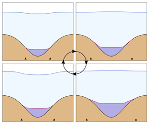
We consider a body of water beneath an ice sheet in the plane. We denote the spatial coordinate by $\boldsymbol {x}=(x,z)$. We assume the lower boundary of the ice is described by a function $s(x,t)$ that is bounded below by the bed, $\beta (x)$. We define $h(x,t)$ to be the surface elevation of the ice sheet. The ice-filled domain is defined by

(2.1)\begin{equation} \varOmega = \left\{(x,z):\; |x| < L/2,\ s(x,t)< z < h(x,t)\right\}, \end{equation}

for a constant length $L$. As we are mainly concerned with modelling ice flow near the grounding lines, the length $L$ is arbitrary but much smaller than the length of the ice sheet. We let $\varGamma _w$ and $\varGamma _b$ be the ice–water and ice–bed surfaces, respectively. These boundaries are defined by

(2.2)\begin{gather} \varGamma_w = \{(x,z)\in\partial\varOmega: \ z=s(x,t)>\beta(x) \}, \end{gather}

(2.3)\begin{gather}\varGamma_b = \{(x,z)\in\partial\varOmega: \ z=s(x,t)=\beta(x) \}, \end{gather}

(2.4)\begin{gather}\varGamma_s = \varGamma_w\cup\varGamma_b, \end{gather}

where $\varGamma _s$ denotes the entirety of the lower boundary. Grounding lines exist where the ice–water and ice–bed boundaries meet. We let the minimum and maximum grounding-line positions be $x_-(t)$ and $x_+(t)$, respectively. We use $x_\pm$ to collectively refer to both grounding lines. We assume that the subglacial-lake water is not connected to the surface, although this is not true for all glacial lakes. The model geometry for both settings is illustrated in figure 1.

Figure 1. (a) Model geometry for the marine ice-sheet problem, highlighting the boundaries defined in §§ 2.1 and 2.4. The horizontal inflow speed is noted by $u_0>0$. (b) Model geometry for the subglacial-lake problem. We consider zero inflow and outflow ($u_0=0$) in this setting.

2.2. Ice flow

Here, we outline the ice-flow component of the model. We let $\boldsymbol {u}$ be the ice velocity, $p$ the ice pressure, $\rho _i$ the ice density and $\eta$ the ice viscosity. We denote the horizontal and vertical components of a vector $\boldsymbol {v}$ by $v_x$ and $v_z$, respectively. We assume that ice deforms as an incompressible viscous fluid subject to the Stokes equations

(2.5)\begin{gather} -\boldsymbol{\nabla} \boldsymbol{\cdot} \boldsymbol{\sigma}(\boldsymbol{u},p) = \rho_i\boldsymbol{g}, \end{gather}

(2.6)\begin{gather}\boldsymbol{\nabla} \boldsymbol{\cdot} \boldsymbol{u} = 0, \end{gather}

where $\boldsymbol {g}=g[0,-1]^{\mathrm {T}}$ is gravitational acceleration with magnitude $g$. Momentum conservation and incompressibility are ensured through (2.5) and (2.6), respectively. The stress is related to pressure and velocity through

(2.7)\begin{equation} \boldsymbol{\sigma}(\boldsymbol{u},p)={-}p\boldsymbol{\mathsf{I}} + 2\eta(\boldsymbol{u}) \boldsymbol{\mathsf{D}}(\boldsymbol{u}), \end{equation}

where

(2.8)\begin{equation} \boldsymbol{\mathsf{D}}(\boldsymbol{u}) = \tfrac{1}{2}\left[\boldsymbol{\nabla} \boldsymbol{u} + (\boldsymbol{\nabla} \boldsymbol{u})^{\mathrm{T}} \right] \end{equation}

is the strain rate and $\boldsymbol{\mathsf{I}}$ is the identity matrix. Throughout, we use the Frobenius norm $|\boldsymbol{\mathsf{D}}| = \sqrt {\boldsymbol{\mathsf{D}}\boldsymbol {:}\boldsymbol{\mathsf{D}}}$ for tensors. Defining $n\geqslant 1$ to be the stress exponent and $A>0$ the ice softness, we use Glen's law to relate the viscosity to the strain rate through the equation

(2.9)\begin{equation} \eta(\boldsymbol{u}) = \tfrac{1}{2}B(|\boldsymbol{\mathsf{D}}(\boldsymbol{u})|^2 + \delta)^{({r-2})/{2}}, \end{equation}

where $r=1+1/n$ and $B=2^{({n-1})/{2n}}A^{-{1}/{n}}$ are flow law parameters (Glen Reference Glen1955; Cuffey & Paterson Reference Cuffey and Paterson2010). The parameter $\delta \ll 1$ is used to prevent infinite viscosity at zero strain rate in numerical simulations (Jouvet & Rappaz Reference Jouvet and Rappaz2011; Helanow & Ahlkrona Reference Helanow and Ahlkrona2018). While ice has a viscoelastic rheology on the tidal time scales explored in § 4.1, we consider the purely viscous rheology here to illustrate the numerical method and provide a point of comparison for studies that include elasticity.

The evolution of the upper and lower surfaces are governed by the kinematic equations

(2.10)\begin{gather} \frac{\partial h}{\partial t}(x,t) = \sqrt{1+\left(\frac{\partial h}{\partial x}\right)^2}\, u_n(x,h,t), \end{gather}

(2.11)\begin{gather}\frac{\partial s}{\partial t}(x,t) ={-}\sqrt{1+\left(\frac{\partial s}{\partial x}\right)^2} \, u_n(x,s,t), \end{gather}

where

(2.12)\begin{equation} u_n = \boldsymbol{u}\boldsymbol{\cdot}\boldsymbol{n}|_{\partial\varOmega} \end{equation}

is the normal component of the velocity on the boundary and $\boldsymbol {n}$ is the outward-pointing unit normal to the boundary (Durand et al. Reference Durand, Gagliardini, De Fleurian, Zwinger and Le Meur2009a; Schoof Reference Schoof2011). We neglect mass change at the surface (e.g. accumulation or ablation) and bed (e.g. melting or freezing) in (2.10) and (2.11), respectively, in order to focus on the mechanical contact problems.

2.3. Water pressure and volume change

We assume that both the ocean and subglacial lake are hydrostatic. We let $p_w$ be the water pressure at the ice–water interface, with $p_w^{o}$ and $p_w^{l}$ denoting the particular expressions for the ocean and subglacial lake, respectively. For marine ice sheets, the hydrostatic water pressure is $p_w^o = \rho _w g (\ell -s)$, where $\ell$ is sea level. However, using the elevation $s$ computed from the velocity solution at the previous time step is numerically unstable (Durand et al. Reference Durand, Gagliardini, De Fleurian, Zwinger and Le Meur2009a). We approximate $s$ at the current time step by applying the backward Euler method to (2.11) under the assumption of small gradients, $({\partial s}/{\partial x})^2\ll 1$, to yield

(2.13)\begin{equation} s_*(x,t) = s(x,t-\Delta t) - (\Delta t) u_n (x,s,t), \end{equation}

where $\Delta t$ is the time-step size. Using the approximation $s_*$, the sub-shelf water pressure becomes

(2.14)\begin{equation} p_{w}^o(x,s,t) = \rho_w g (\ell(t)-s_*(x,t)) . \end{equation}

Subglacial lakes have finite volume that can change considerably over time. The subglacial-lake volume $\mathcal {V}$ evolves according to

(2.15)\begin{equation} \dot{\mathcal{V}}(t) ={-}\int_{\varGamma_s}u_n\,\mathrm{d}\boldsymbol{s}. \end{equation}

For a prescribed volume change rate, equation (2.15) acts as an integral constraint on the normal component of the velocity at the base. In contrast, the marine ice-sheet problem does not have a constraint such as (2.15) because the ocean volume is larger than the sub-shelf cavity volume. In the marine case, the water volume change is instead controlled by the ice-flow response to water pressure variations, analogous to models of subglacial cavitation (Schoof Reference Schoof2005; Gagliardini et al. Reference Gagliardini, Cohen, Råback and Zwinger2007).

We assume that subglacial-lake water is not connected to the surface, so there is no datum where water pressure is known a priori. Assuming hydrostatic balance ($\boldsymbol {\nabla } p_w = \rho _w \boldsymbol {g}$), the expression for water pressure is only determined up to a constant. Therefore, we choose to express the subglacial-lake water pressure as $p_w^{l} = \rho _wg (\bar {s}-s) + \bar {p}_w,$ where $\bar {s}$ and $\bar {p}_w$ are the means of $s$ and $p_w^{l}$ over $(x_-,x_+)$. Although we expect that the water pressure is near the cryostatic pressure as assumed in previous models, determining $\bar {p}_w$ is part of the solution to the problem (Pattyn Reference Pattyn2008; Gudlaugsson et al. Reference Gudlaugsson, Humbert, Kleiner, Kohler and Andreassen2016). In the following, we show that approximating $\bar {p}_w$ by the mean cryostatic pressure is accurate within a few kilopascals. However, the utility of leaving $\bar {p}_w$ undetermined is that it acts as a Lagrange multiplier that enforces the volume-change constraint (§ 3.1).

We also require a numerically stable approximation of the subglacial-lake water pressure. We may replace $\varGamma _s$ with $\varGamma _w$ in (2.15) by applying Leibniz's rule to $\mathcal {V}=\int _{x_-}^{x_+}s-b\,\mathrm {d} x$ if $x_-(t)$ and $x_+(t)$ are continuously differentiable. Although this smoothness assumption may not hold in general, we use it as an approximation in the stabilising scheme. Taking the mean of (2.13), we approximate $\bar {s}(t)$ at the current time step by

(2.16)\begin{equation} \bar{s}_*(t) = \bar{s}(t-\Delta t) + (\Delta t) \dot{\mathcal{V}}/|\varGamma_w|, \end{equation}

where we have assumed $-\int _{\varGamma _w} u_n\,\mathrm {d}\boldsymbol {s}\approx \dot {\mathcal {V}}$ and denoted the measure of $\varGamma _w$ by $|\varGamma _w|$. Using the approximations (2.13) and (2.16), we arrive at the expression for subglacial-lake water pressure

(2.17)\begin{equation} p_{w}^l(x,s,t) = \rho_wg (\bar{s}_*(t)-s_*(x,t)) + \bar{p}_w(t) . \end{equation}

We omit time arguments for brevity.

2.4. Boundary conditions

Stress continuity at the ice–water boundary implies

(2.18)\begin{equation} \boldsymbol{\sigma} \boldsymbol{n} ={-}p_w\boldsymbol{n} \quad \mathrm{on}\ \varGamma_w, \end{equation}

where $p_w$ is given by either (2.14) or (2.17), depending on the setting. Equation (2.18) implies that the shear stress vanishes on the ice–water boundary. We assume a stress-free condition at the ice–air interface, which requires that

(2.19)\begin{equation} \boldsymbol{\sigma} \boldsymbol{n} = \boldsymbol{0} \quad \mathrm{on}\ z=h(x,t). \end{equation}

On the inflow and outflow boundaries, we consider two types of boundary conditions (figure 1). First, we prescribe a uniform horizontal velocity and zero vertical shear stress

(2.20)\begin{equation} \left. \begin{array}{l@{}} u_x = u_0 \\ \boldsymbol{\mathsf{T}}\boldsymbol{\sigma} \boldsymbol{n} = \boldsymbol{0} \end{array} \right\} \quad \mathrm{on}\ \varGamma_{D}, \end{equation}

where $u_0\geqslant 0$ is the horizontal flow speed and $\boldsymbol{\mathsf{T}}= \boldsymbol{\mathsf{I}}-\boldsymbol {n} \boldsymbol {n}^{\mathrm {T}}$ is an orthogonal projection on to the boundary. Here $\varGamma _D$ coincides with the inflow boundary in the case $u_0 > 0$ (marine case), or both the inflow and outflow boundaries when $u_0=0$ (subglacial-lake case). In the marine case ($u_0> 0$), we assume a cryostatic normal-stress condition of the form

(2.21)\begin{equation} \boldsymbol{\sigma} \boldsymbol{n} ={-}\rho_i g (h-z)\boldsymbol{n} \quad \mathrm{on}\ \varGamma_{N}, \end{equation}

where $\varGamma _N$ coincides with the outflow boundary. These inflow and outflow conditions are noted in figure 1.

In the marine case, equating the normal stresses

(2.22)\begin{equation} {\sigma}_n ={-}\boldsymbol{n}\boldsymbol{\cdot}\boldsymbol{\sigma}\boldsymbol{n}|_{\partial\varOmega} \end{equation}

associated with (2.18) and (2.21), where $\varGamma _N$ and $\varGamma _w$ meet (see figure 1a) leads to the flotation condition

(2.23)\begin{equation} h= s+\frac{\rho_w}{\rho_i}(\ell-s) \quad ({\equiv} h_f) \end{equation}

in the limit $\Delta t\to 0$ ($s_*\to s$). We confirm in what follows that the ice-surface elevation near the outflow boundary remains close to $h_f$ (§ 4.1).

On the ice–bed boundary, we assume a sliding law of the form

(2.24)\begin{equation} \boldsymbol{\mathsf{T}}\boldsymbol{\sigma}\boldsymbol{n}+ \alpha (\boldsymbol{u}) \boldsymbol{\mathsf{T}}\boldsymbol{u} = \boldsymbol{0} \quad \mathrm{on}\ \varGamma_b \end{equation}

with friction $\alpha$ given by

(2.25)\begin{equation} \alpha(\boldsymbol{u}) = C(|\boldsymbol{\mathsf{T}}\boldsymbol{u}|^2 + \delta)^{({r-2})/{2}}, \end{equation}

where $C> 0$ is the friction coefficient and $|\boldsymbol {a}|$ denotes the Euclidean norm of a vector $\boldsymbol {a}$ (Weertman Reference Weertman1957; Kamb Reference Kamb1970). In the friction law (2.25), we assume the same value of regularisation parameter $\delta$ as in the flow law (2.9).

There are three possibilities for the normal stress ${\sigma }_n$ and normal component of the velocity $u_n$ at the ice–bed boundary. The first possibility is that the normal stress exceeds the water pressure ($\sigma _n >p_w$) and the ice is not lifted off of the bed ($u_n=0$). The second possibility is that the ice is lifted from the bed ($u_n<0$) and the normal stress equals the water pressure ($\sigma _n=p_w$) (Durand et al. Reference Durand, Gagliardini, De Fleurian, Zwinger and Le Meur2009a; Schoof Reference Schoof2011). The third possibility is that the normal stress reaches the water pressure ($\sigma _n=p_w$), but the ice is not lifted from the bed ($u_n=0$). These three cases are represented by either

(2.26)\begin{equation} \left. \begin{array}{c@{}} {\sigma}_n \geqslant p_w \\ u_n = 0 \end{array}\right\} \quad \mathrm{or} \quad \left. \begin{array}{c@{}} {\sigma}_n = p_w \\ u_n \leqslant 0 \end{array}\right\} \quad \mathrm{on} \ \varGamma_b. \end{equation}

The two sets of conditions in (2.26) are equivalent to

(2.27)\begin{equation} \left. \begin{array}{c@{}} {\sigma}_n \geqslant p_w \\ u_n \leqslant 0 \\ ({\sigma}_n - p_w)u_n = 0 \end{array}\right\} \quad \mathrm{on}\ \varGamma_b. \end{equation}

The contact conditions (2.27) are analogous to those in the Signorini problem from elasticity (Kikuchi & Oden Reference Kikuchi and Oden1988). We refer to the condition $u_n \leqslant 0$ as bed impenetrability.

3.1. Derivation of mixed formulations

We now derive weak formulations of the models. We let $V$ and $Q$ be appropriate function spaces for the velocity and pressure, respectively (Appendix A.1). We define the set of admissible velocity fields by

(3.1)\begin{equation} {K} = \{\boldsymbol{v}\in V: \ v_n|_{\varGamma_b} \leqslant 0 \ \mathrm{and}\ v_x|_{\varGamma_{D}} = u_0 \}, \end{equation}

which is a closed, convex subset of $V$. We let $\boldsymbol {v}\in K$ be an arbitrary test function, multiply (2.5) by $\boldsymbol {v}-\boldsymbol {u}$ and integrate by parts to obtain

(3.2)\begin{equation} \int_{\varOmega}2\eta(\boldsymbol{u})\boldsymbol{\mathsf{D}}(\boldsymbol{u})\boldsymbol{:} \boldsymbol{\mathsf{D}}(\boldsymbol{v}-\boldsymbol{u}) - \rho_i\boldsymbol{g}\boldsymbol{\cdot}(\boldsymbol{v}-\boldsymbol{u}) -p\boldsymbol{\nabla}\boldsymbol{\cdot} (\boldsymbol{v}-\boldsymbol{u}) \, \mathrm{d}\boldsymbol{x} - \int_{\partial \varOmega} \boldsymbol{\sigma} \boldsymbol{n}\boldsymbol{\cdot} (\boldsymbol{v}-\boldsymbol{u}) \, \mathrm{d}\boldsymbol{s}=0, \end{equation}

where we used the identity $\boldsymbol{\mathsf{D}}(\boldsymbol {u})\boldsymbol {:}\boldsymbol {\nabla }(\boldsymbol {v}-\boldsymbol {u}) =\boldsymbol{\mathsf{D}}(\boldsymbol {u})\boldsymbol {:}\boldsymbol{\mathsf{D}}(\boldsymbol {v}-\boldsymbol {u})$.

We turn our attention to the boundary integral over $\varGamma _b$. Using $\boldsymbol {\sigma } \boldsymbol {n} = \boldsymbol{\mathsf{T}}\boldsymbol {\sigma }\boldsymbol {n} - {\sigma }_n \boldsymbol {n}$, the sliding law (2.24) and the identity $\boldsymbol{\mathsf{T}}\boldsymbol {u}\boldsymbol {\cdot } (\boldsymbol {v}-\boldsymbol {u})=\boldsymbol{\mathsf{T}}\boldsymbol {u}\boldsymbol {\cdot } \boldsymbol{\mathsf{T}}(\boldsymbol {v}-\boldsymbol {u})$ (since $\boldsymbol{\mathsf{T}}$ is an orthogonal projection), we obtain

(3.3)\begin{equation} - \int_{\varGamma_b} \boldsymbol{\sigma} \boldsymbol{n}\boldsymbol{\cdot} (\boldsymbol{v}-\boldsymbol{u}) \, \mathrm{d}\boldsymbol{s} = \int_{\varGamma_b} \alpha(\boldsymbol{u})\boldsymbol{\mathsf{T}}\boldsymbol{u}\boldsymbol{\cdot} \boldsymbol{\mathsf{T}}(\boldsymbol{v}-\boldsymbol{u}) \, \mathrm{d}\boldsymbol{s} + \int_{\varGamma_b} {\sigma}_n(v_n-u_n) \, \mathrm{d}\boldsymbol{s}. \end{equation}

The contact conditions (2.27) and $v_n|_{\varGamma _b}\leqslant 0$ imply that

(3.4)\begin{equation} \int_{\varGamma_b} {\sigma}_n(v_n-u_n) \, \mathrm{d}\boldsymbol{s} \leqslant \int_{\varGamma_b} p_w(v_n-u_n) \,\mathrm{d}\boldsymbol{s}. \end{equation}

Combining inequality (3.4) with (3.2)–(3.3) and the boundary conditions (2.18)–(2.21), we obtain the variational inequality

(3.5)\begin{align} &\int_{\varOmega} \left[ 2\eta(\boldsymbol{u})\boldsymbol{\mathsf{D}}(\boldsymbol{u})\boldsymbol{:}\boldsymbol{\mathsf{D}}(\boldsymbol{v}-\boldsymbol{u}) - \rho_i\boldsymbol{g}\boldsymbol{\cdot}(\boldsymbol{v}-\boldsymbol{u}) -p\boldsymbol{\nabla}\boldsymbol{\cdot} (\boldsymbol{v}-\boldsymbol{u})\right] \mathrm{d}\boldsymbol{x} + \int_{\varGamma_s} p_w (v_n-u_n) \, \mathrm{d}\boldsymbol{s} \nonumber\\ &\quad+\int_{\varGamma_b} \alpha(\boldsymbol{u})\boldsymbol{\mathsf{T}}\boldsymbol{u}\boldsymbol{\cdot} \boldsymbol{\mathsf{T}}(\boldsymbol{v}-\boldsymbol{u}) \, \mathrm{d}\boldsymbol{s} +\int_{\varGamma_{N}} \rho_i g (h-z) (v_n-u_n) \, \mathrm{d}\boldsymbol{s} \geqslant 0. \end{align}

To simplify notation, we write

(3.6)\begin{align} \mathcal{F}(\boldsymbol{u},\boldsymbol{v}) &= \int_{\varOmega} \left[ 2\eta(\boldsymbol{u})\boldsymbol{\mathsf{D}}(\boldsymbol{u})\boldsymbol{:}\boldsymbol{\mathsf{D}}(\boldsymbol{v}) - \rho_i\boldsymbol{g}\boldsymbol{\cdot}\boldsymbol{v}\right] \mathrm{d}\boldsymbol{x} +\int_{\varGamma_b} \alpha(\boldsymbol{u})\boldsymbol{\mathsf{T}}\boldsymbol{u}\boldsymbol{\cdot} \boldsymbol{\mathsf{T}}\boldsymbol{v} \, \mathrm{d}\boldsymbol{s}\nonumber\\ &\quad +\int_{\varGamma_{N}}\rho_i g (h-z) v_n \, \mathrm{d}\boldsymbol{s} \end{align}

(3.7)\begin{align} b_\varOmega(q,\boldsymbol{u}) &= \int_\varOmega q\boldsymbol{\nabla}\boldsymbol{\cdot}\boldsymbol{u} \, \mathrm{d}\boldsymbol{x}, \end{align}

for $\boldsymbol {u},\boldsymbol {v}\in V$ and $q\in Q$, which constitute the usual weak forms in Stokes ice-flow models. We also define

(3.8)\begin{gather} \mathcal{P}_{w}^o (\boldsymbol{u},\boldsymbol{v}) = \rho_w g \int_{\varGamma_s} \left[ \ell - s + (\Delta t) u_n \right] v_n \,\mathrm{d}\boldsymbol{s}, \end{gather}

(3.9)\begin{gather}\mathcal{P}_{w}^l(\boldsymbol{u},\boldsymbol{v}) = \rho_wg \int_{\varGamma_s} [ \bar{s} - s + (\Delta t) (u_n + {\dot{\mathcal{V}}}/{|\varGamma_w|} )] v_n \,\mathrm{d}\boldsymbol{s}, \end{gather}

(3.10)\begin{gather}b_\varGamma (q_w,\boldsymbol{u}) ={-} \int_{\varGamma_s} q_wu_n\, \mathrm{d}\boldsymbol{s}, \end{gather}

for $\boldsymbol {u},\boldsymbol {v}\in V$ and $q_w\in \mathbb {R}$, which originate from the weak forms of the ocean water pressure (2.14), subglacial-lake water pressure (2.17) and lake volume-change constraint (2.15), respectively. In (3.8) and (3.9), $s$ and $\bar {s}$ are known from the previous time step (§ 2.3).

We supplement inequality (3.5) with the weak form of incompressibility (3.7) and sub-shelf water pressure (3.8) to arrive at the mixed variational problem for marine ice sheets. We seek $(\boldsymbol {u},p)\in K \times Q$ such that

(3.11)\begin{equation} \left\{\begin{array}{@{}ll} \mathcal{F}(\boldsymbol{u},\boldsymbol{v}-\boldsymbol{u}) + \mathcal{P}_{w}^o(\boldsymbol{u},\boldsymbol{v}-\boldsymbol{u}) - b_\varOmega(p,\boldsymbol{v}-\boldsymbol{u}) \geqslant 0 \\ b_\varOmega(q,\boldsymbol{u}) = 0 \end{array}\right.\end{equation}

for all $(\boldsymbol {v},q)\in K\times Q$. Similarly, the variational problem for subglacial lakes is to find $(\boldsymbol {u},p,\bar {p}_w)\in K \times Q\times \mathbb {R}$ such that

(3.12)\begin{equation} \left\{ \begin{array}{@{}ll} \mathcal{F}(\boldsymbol{u},\boldsymbol{v}-\boldsymbol{u}) + \mathcal{P}_{w}^l(\boldsymbol{u},\boldsymbol{v}-\boldsymbol{u}) - b_\varOmega(p,\boldsymbol{v}-\boldsymbol{u}) - b_\varGamma(\bar{p}_w,\boldsymbol{v}-\boldsymbol{u}) \geqslant 0 \\ b_\varOmega(q,\boldsymbol{u}) + b_\varGamma(q_w,\boldsymbol{u}) = q_w\dot{\mathcal{V}} \end{array}\right.\end{equation}

for all $(\boldsymbol {v},q,q_w)\in K \times Q \times \mathbb {R}$. In deriving (3.12), we used the subglacial-lake volume-change constraint (2.15) and the expression for water pressure (2.17). The form of (3.12) shows that the mean water pressure $\bar {p}_w$ acts as a Lagrange multiplier that enforces the volume-change constraint, analogous to $p$ enforcing incompressibility; we elaborate on this in the context of the penalty formulation in § 3.3.

3.2. Minimisation formulation

We now introduce minimisation formulations of problems (3.11) and (3.12) that justify the penalty methods discussed in the following section. We denote the set of divergence-free admissible velocity fields that obey the volume-change constraint by

(3.13)\begin{equation} K_\star{=} \{\boldsymbol{u}\in K:\ b_\varOmega(q,\boldsymbol{u}) + b_\varGamma(q_w,\boldsymbol{u})=q_w\dot{\mathcal{V}} \ \mathrm{for}\ \mathrm{all}\ (q,q_w)\in Q\times \mathbb{R} \}, \end{equation}

which is a closed, convex subset of $V$ (Appendix A.2). On this subset, the mixed variational problem (3.12) reduces to finding $\boldsymbol {u}\in K_\star$ such that

(3.14)\begin{equation} \mathcal{F}(\boldsymbol{u},\boldsymbol{v}-\boldsymbol{u}) + \mathcal{P}_w^l(\boldsymbol{u},\boldsymbol{v}-\boldsymbol{u}) \geqslant 0 \end{equation}

for all $\boldsymbol {v}\in K_\star$. For the sake of clarity, we set the regularisation parameter to $\delta =0$ in the flow law (2.9) and sliding law (2.25). The results below still hold for $\delta >0$ (Jouvet & Rappaz Reference Jouvet and Rappaz2011). The left side of (3.14) is the Gâteaux derivative of the functional

(3.15)\begin{align} \mathcal{J}(\boldsymbol{v}) &= \int_{\varOmega} \frac{B}{r}|\boldsymbol{\mathsf{D}}(\boldsymbol{v})|^{r} -\rho_i\boldsymbol{g}\boldsymbol{\cdot}\boldsymbol{v} \, \mathrm{d}\boldsymbol{x} + \int_{\varGamma_b} \frac{C}{r} |\boldsymbol{\mathsf{T}}\boldsymbol{v}|^{r} \, \mathrm{d}\boldsymbol{s} + \int_{\varGamma_{N}} \rho_i g (h-z) v_n \, \mathrm{d}\boldsymbol{s} \nonumber\\ &\quad + \rho_w g\int_{\varGamma_s} \gamma_1 v_n^2 + \left(\gamma_2-s\right) v_n \,\mathrm{d}\boldsymbol{s} \end{align}

in the direction $\boldsymbol {v}-\boldsymbol {u}$, where $\gamma _1 = {\Delta t}/{2}$ and $\gamma _2 = {\dot {\mathcal {V}}\Delta t}/{|\varGamma _w|}+ \bar {s}$.

The problem of minimising $\mathcal {J}$ (3.15) over $K_\star$ is equivalent to solving variational inequality (3.14) (Kikuchi & Oden Reference Kikuchi and Oden1988, Theorem 3.7). The functional $\mathcal {J}$ is convex, continuous and coercive (Appendix A.2). These properties ensure that a minimiser $\boldsymbol {u}\in {K}_\star$ of $\mathcal {J}$ exists (Ekeland & Temam Reference Ekeland and Temam1999, Proposition 1.2). Uniqueness follows from the strict convexity of $\mathcal {J}$ (Chen, Gunzburger & Perego Reference Chen, Gunzburger and Perego2013, Lemmas 9 and 12). Therefore, there exists a unique solution $\boldsymbol {u}$ to the reduced problem (3.14). Existence and uniqueness of the corresponding pressures $p$ and $\bar {p}_w$ in the mixed formulation (3.12) follow from an inf–sup condition on the constraint operators $b_\varOmega$ and $b_\varGamma$ (Appendix A.3). Existence and uniqueness of solutions to the marine ice-sheet problem follows the same argument applied to the functional $\mathcal {J}$, with $\gamma _2 =\ell$, over the set of divergence-free admissible velocity fields.

3.3. Penalty formulation

Working with the set $K$ is inconvenient for arbitrary bed geometry. Instead, we introduce a penalty formulation that is posed over $V$. To enforce the impenetrability constraint, we introduce the penalty functional

(3.16)\begin{equation} \varPi(\boldsymbol{v}) = \int_{\varGamma_b} \tfrac{1}{2}\left(v_n^2 + v_n|v_n| \right) \mathrm{d}\boldsymbol{s}. \end{equation}

The Gâteaux derivative of $\varPi$ at $\boldsymbol {u}$ in a direction $\boldsymbol {v}$ is

(3.17)\begin{equation} \varPi'(\boldsymbol{u},\boldsymbol{v}) = \int_{\varGamma_b} \left(u_n + |u_n| \right)v_n \, \mathrm{d}\boldsymbol{s}. \end{equation}

$\varPi$ and $\varPi '$ are non-zero only when impenetrability is violated (i.e.when $u_n>0$). Therefore, $({1}/{\varepsilon })\varPi$ (and $({1}/{\varepsilon })\varPi '$) penalises $u_n>0$ when the penalty parameter $\varepsilon$ is chosen to be small. We seek $\boldsymbol {u}\in V$ that minimises the penalised functional

(3.18)\begin{equation} \mathcal{J}_\varepsilon(\boldsymbol{v}) = \mathcal{J}(\boldsymbol{v}) + \frac{1}{\varepsilon}\varPi(\boldsymbol{v}), \end{equation}

and satisfies the relevant equality constraints, depending on the problem. Minimisers of $\mathcal {J}_\varepsilon$ converge weakly to minimisers of $\mathcal {J}$ as $\varepsilon \to 0$, justifying the numerical method (Kikuchi & Oden Reference Kikuchi and Oden1988, Theorem 3.15).

To enforce the equality constraints, we introduce the Lagrangian for the marine problem

(3.19)\begin{equation} \mathcal{L}^o(\boldsymbol{v},q) = \mathcal{J}_\varepsilon(\boldsymbol{v}) - b_\varOmega(q,\boldsymbol{v}), \end{equation}

and for lake problem

(3.20)\begin{equation} \mathcal{L}^l(\boldsymbol{v},q,q_w) = \mathcal{J}_\varepsilon(\boldsymbol{v}) - b_\varOmega(q,\boldsymbol{v})- b_\varGamma(q_w,\boldsymbol{v}) + q_w\dot{\mathcal{V}}, \end{equation}

where the pressures $(q,q_w)\in Q\times \mathbb {R}$ have been reintroduced as Lagrange multipliers. The solutions $(\boldsymbol {u},p)$ to the marine problem and $(\boldsymbol {u},p,\bar {p}_w)$ to the lake problem are saddle points of (3.19) and (3.20), respectively. We obtain the penalty formulations of (3.11) and (3.12) by taking Gâteaux derivatives of these Lagrangians (Kikuchi & Oden Reference Kikuchi and Oden1988, Theorem 3.13).

For the marine ice-sheet model, the penalised problem is to find $(\boldsymbol {u},p)\in V\times Q$, satisfying the Dirichlet condition, such that

(3.21)\begin{equation} \left\{\begin{array}{@{}ll} \mathcal{F}(\boldsymbol{u},\boldsymbol{v}) + \mathcal{P}_w^o(\boldsymbol{u},\boldsymbol{v}) - b_\varOmega(p,\boldsymbol{v}) + \dfrac{1}{\varepsilon}\varPi'(\boldsymbol{u},\boldsymbol{v}) = 0 \\ b_\varOmega(q,\boldsymbol{u}) = 0 \end{array}\right.\end{equation}

for all $(\boldsymbol {v},q)\in V_D\times Q$, where $V_D=\{\boldsymbol {v}\in V:\ v_x|_{\varGamma _D}=0 \}$. Similarly, the subglacial-lake problem reduces to finding $(\boldsymbol {u},p,\bar {p}_w)\in V\times Q\times \mathbb {R}$ such that

(3.22)\begin{equation} \left\{ \begin{array}{@{}ll} \mathcal{F}(\boldsymbol{u},\boldsymbol{v}) + \mathcal{P}_w^l(\boldsymbol{u},\boldsymbol{v}) - b_\varOmega(p,\boldsymbol{v}) - b_\varGamma(\bar{p}_w,\boldsymbol{v}) + \dfrac{1}{\varepsilon}\varPi'(\boldsymbol{u},\boldsymbol{v}) = 0 \\ b_\varOmega(q,\boldsymbol{u}) + b_\varGamma(q_w,\boldsymbol{u}) = q_w\dot{\mathcal{V}} \end{array}\right.\end{equation}

for all $(\boldsymbol {v},q,q_w)\in V_D\times Q\times \mathbb {R}$. Variational problems (3.21) and (3.22) readily extend to three spatial dimensions; the details depend on the additional boundary conditions on the side walls of the domain, that must be chosen.

3.4. Numerical implementation

At each time step, we solve variational problem (3.21) or (3.22) with the finite-element package FEniCS (Logg, Mardal & Wells Reference Logg, Mardal and Wells2012; Alnæs et al. Reference Alnæs, Blechta, Hake, Johansson, Kehlet, Logg, Richardson, Ring, Rognes and Wells2015). We use the Taylor–Hood element for velocity and pressure (Jouvet & Rappaz Reference Jouvet and Rappaz2011). In the subglacial-lake case, the Taylor–Hood element is augmented with a Lagrange multiplier for $\bar {p}_w,q_w\in \mathbb {R}$, constituting a single additional global degree of freedom. We update the free surfaces $h$ and $s$ using (2.10) and (2.11) and the velocity solution, moving the boundary nodes of the mesh to obtain the new domain. The geometric constraint $s\geqslant \beta$ is then enforced explicitly. The interior nodes of the mesh are smoothed using the ALE (arbitrary Lagrangian–Eulerian) class in DOLFIN (Logg & Wells Reference Logg and Wells2010; Logg et al. Reference Logg, Mardal and Wells2012). For the simulations discussed in § 4, we set the element width to 250 m at the upper surface and refine it to $\Delta x = 12.5\ \textrm {m}$ at the lower surface. We choose the regularisation parameter $\delta =10^{-15}$, flow law coefficient $B = 8.6 \times 10^{7}\ \textrm {Pa}\ \textrm {s}^{1/3}$, flow law exponent $r=4/3$, friction coefficient $C = 10^{5}\ \textrm {Pa}\ \textrm {s}^{1/3}\ \textrm {m}^{-1/3}$ and penalty parameter $\varepsilon = 10^{-13}$. The time-step sizes $\Delta t$ for the different problems are provided subsequently. These parameters provide well-resolved and converged solutions (Appendix B.1).

In general, the true grounding-line positions exist between the mesh nodes. The numerical grounding-line positions depend on how the discretised ice–water (2.2) and ice–bed (2.3) boundaries are defined. Here, the discretised ice–bed boundary is defined as all element edges satisfying $s-\beta \leqslant \tau$ for a specified numerical tolerance $\tau$, 1 mm for all examples herein. The discretised ice–water boundary includes all edges on the lower boundary satisfying $s-\beta > \tau$ and the edges where the true grounding lines exist (i.e. where $s-\beta -\tau$ changes sign). This choice of discretisation corresponds to the ‘last-grounded’ scheme in Gagliardini et al. (Reference Gagliardini, Brondex, Gillet-Chaulet, Tavard, Peyaud and DURAND2016). Sub-grid parameterisations of the transition between these boundaries have been developed (Seroussi et al. Reference Seroussi, Morlighem, Larour, Rignot and Khazendar2014; Cheng et al. Reference Cheng, Lötstedt and von Sydow2020). We do not explore these schemes here because they introduce additional terms in the weak forms that depend on the grounding-line positions. For plotting and convergence testing, we estimate the true grounding-line positions by linear interpolation between the mesh nodes. Throughout, we plot the interpolated positions rather than the adjacent mesh nodes where the discretised ice–water and ice–bed boundaries meet.

Verification and validation of the numerical model are established by providing a known subglacial-lake volume change rate. The computed results can then be compared with the true volume change and, in some cases, an expected grounding-line migration rate. Using this approach, we discuss convergence of the numerical method with decreasing $\varepsilon$, $\Delta t$ and $\Delta x$ (Appendix B.1). We provide a second benchmark test for validation that is based on an expected rate of grounding-line migration for a slow-filling triangular lake (Appendix B.2). For the marine problem, satisfaction of the flotation condition (2.23) near the outflow boundary is also a useful validation measure (figures 2 and 3). The code is openly available as an archived Git repository (Stubblefield Reference Stubblefield2020, doi:10.5281/zenodo.4302610).

Figure 2. (a) Sea-level change $\Delta \ell = \ell (t)-\ell (0)$, mean ice–air elevation change $\Delta \bar {h} = \bar {h}(t)-\bar {h}(0)$ and mean ice–water elevation change $\Delta \bar {s} = \bar {s}(t)-\bar {s}(0)$ over the course of four tidal cycles, where $\bar {h}$ and $\bar {s}$ denote the mean of $h$ and $s$ over the ice–water boundary. The black diamonds mark the times and relative sea levels associated with the free-surface plots in figure 3. (b) Comparison of the outflow elevation $\Delta h_{{out}} = h(L/2,t)-h(L/2,0)$ with the flotation elevation $\Delta h_f = h_f(t)-h_f(0)$, given by (2.23). (c) Minimum and maximum grounding-line positions over time. An extended grounding zone forms when sea level falls, characterised by the presence of a thin water layer between $x_-$ and $x_+$ (discussed in § 4.1). The extended grounding zone is lost when sea level begins to rise, resulting in a single grounding line. We plot the results for $t\geqslant 5$ days after transients in the grounding-line time series have relaxed.

Figure 3. Plot of free-surface geometry over the course of one tidal cycle, with time increasing from (a–d). The times and relative sea levels are noted in figure 2(a). The initial geometry is depicted by dashed black lines in (a). Sea level $\ell$ is depicted by a dash-dotted green line and the ice-flotation elevation $h_f$ (2.23) is depicted by a dashed purple line. For visualisation, 98 % of the initial sea-level and ice-surface elevation have been subtracted from $\ell$ and $h$, respectively. The reference upper surface elevation is $h_0=500$ m. The sea levels in (b,d) are the same. The colour scheme follows figure 1. The minimum and maximum grounding-line positions $x_\pm$ are noted by black triangles.

4.1. Tidal cycles

Here, we illustrate the grounding-line response to tidal cycles in the marine ice-sheet problem. We consider sinusoidal tidal cycles of the form

(4.1)\begin{equation} \ell(t) = \frac{\rho_i}{\rho_w}h_0 + \sin(2{\rm \pi} t/P), \end{equation}

where the initial ice-shelf surface elevation is $h_0=500\ \textrm {m}$, the period $P$ is a half day and the maximum deviation from mean sea level $({\rho _i}/{\rho _w})h_0$ is $1 m$ (figure 2). We choose a linear bed geometry

(4.2)\begin{equation} \beta(x) ={-}\frac{5x}{L}, \end{equation}

where the length $L=20\ \textrm {km}$. The inflow speed is set to $u_0=1\ \textrm {km}\ \textrm {yr}^{-1}$ on $\varGamma _D$. We assume that the cryostatic condition (2.21) holds on the outflow boundary $\varGamma _N$ (figure 1). To construct appropriate initial free surfaces for the tidal problem, we keep the sea level fixed at $\ell (t)=(\rho _i/\rho _w) h_0$ and evolve the initial conditions $s(x,0) = \max (\beta (x),0)$ and $h(x,0) = h_0$ to time $t=0.35$ yr, using a time-step size of $\Delta t=5\times 10^{-4}\ \textrm {yr}$. The resulting initial ice-sheet profile for the tidal simulation thickens inland from the shelf (figure 3a). For the tidal simulation, we reduce the time step to $\Delta t=2\times 10^{-6}\ \textrm {yr}$ to obtain a similar number of time steps per oscillation period as in the subglacial-lake problem where numerical accuracy has been verified. We explore numerical convergence and accuracy with respect to ($\Delta x, \Delta t$) in Appendix B.1 and demonstrate that these solutions are well resolved in space and time.

The mean elevations of the ice–water interface and overlying ice–air interface closely follow the tidal cycle over time (figure 2a). At the outflow boundary, the ice elevation closely matches the flotation condition (2.23) that results from the stress boundary conditions (figure 2b). The grounding-line response is also periodic in time, migrating roughly 5 km over each cycle (figure 2c). The free-surface geometry over the course of one tidal cycle is shown in figure 3. We provide a movie of the complete simulation in the supporting information (supplementary movie 1). An intriguing feature of this solution is that, for oscillations on a tidal time scale, multiple contact points can form (figure 2c).

The tidal cycle causes flexure in the ice sheet that leads to multiple contact points (figure 4). After high tide, ice begins to make contact with the bed as sea level falls. The strong downward flexure of the floating ice shelf causes an upward flexure inland of the main grounding line $x_+$, which acts like a hinge (figure 4a). Ice is lifted from the bed in a zone adjacent to $x_+$, forming a $\sim$1 mm thick water layer of width $\sim$1 km (figure 4b). We refer to this area of thin separation between ice and bed as the extended grounding zone. The upward flexure is balanced by a slight downward flexure farther inland that causes previously lifted patches of ice to progressively regain contact with the bed (figure 4a). This flexural response causes the thin water layer to migrate seaward behind the main grounding line $x_+$ while decaying in amplitude until low tide (figure 2c).

Figure 4. (a,c) Vertical velocity $u_z$ near the grounding line plotted on the displaced mesh during the falling and rising stages of the tidal cycle. The times are noted in figure 2(a). The instantaneous displacement $\boldsymbol {u}\times \Delta t$ has been exaggerated by a factor of ${\sim }3\times 10^5$ for visualisation. The width and structure of the extended grounding zone are noted in (a). Minimum and maximum grounding-line positions are noted by black triangles. (b,d) Water-layer thickness $s-\beta -\tau$ during the falling and rising stages of the tidal cycle, where $\tau$ is the boundary geometry tolerance parameter defined in § 3.4. (b) shows the $\sim$1 mm thick water layer that forms between $x_-$ and $x_+$. Supplementary movies 2–4 available at https://doi.org/10.1017/jfm.2021.394 show the evolution of the water-layer thickness over the full simulation for a range of numerical parameters.

We show that the extended grounding zone forms for a wide range of mesh spacings in supplementary movie 2 ($\Delta x = 12.5$, $50$ and 100 m), time-step sizes in supplementary movie 3 ($\Delta t=1$, $2$ and 4 min) and boundary geometry tolerances in supplementary movie 4 ($\tau =10^{-2}$, $10^{-3}$ and $10^{-4}\ \textrm {m}$). The width, maximum amplitude and migration speed of the water layer are insensitive to changes in these parameters. Therefore, the extended grounding zone is a robust feature of the solution. When the water layer collapses near low tide, differences between the solutions can occur on the sub-millimetre scale.

After low tide, the extended grounding zone is lost as ice is lifted off the bed by the rising sea (figures 2c, 3b). Only one grounding line exists as sea level rises because a downward flexure occurs inland of $x_+$, balancing the strong upward flexure of the ice shelf (figure 4c,d). The grounding line migrates inland until high tide, when the cycle is completed. The extended grounding zone does not form at longer (e.g.weekly) oscillation periods because the flexural response is absent (supplementary movie 5).

4.2. Subglacial lake filling–draining cycles

Here, we illustrate grounding-line responses to subglacial-lake filling–draining cycles. Motivated by observations and modelling studies of sub-decadal cycles, we use a volume change rate $\dot {\mathcal {V}}$ obtained from a smoothed sawtooth volume-change time series with a period of one year (Fowler Reference Fowler2009; Kingslake Reference Kingslake2015; Siegfried & Fricker Reference Siegfried and Fricker2018; Stubblefield et al. Reference Stubblefield, Creyts, Kingslake and Spiegelman2019). The volume change $\mathcal {V}$ is shown in figure 5(a). We assume that the subglacial lake exists in a topographic low point on the bed beneath an ice slab of length $L=10$ km. Therefore, we let the bed topography be a Gaussian

(4.3)\begin{equation} \beta(x) ={-} 10\exp\left({-}16\frac{x^2}{L^2}\right). \end{equation}

We choose an initial lower surface given by $s(x,0) = \max (\beta (x),-5\ \mathrm {m}),$ and a uniform initial upper-surface elevation of $h(x,0)\equiv 1$ km (figure 6a). We set the horizontal inflow and outflow speeds to $u_0=0$ on $\varGamma _D = \{|x|=L/2\}$ so that $\varGamma _N = \emptyset$ (figure 1). We choose a time-step size of $\Delta t=5\times 10^{-4}$ yr.

Figure 5. (a) Computed lake volume change $\mathcal {V}/\mathcal {V}_0$ compared with the exact volume change $\mathcal {V}_{true}/\mathcal {V}_0$, where $\mathcal {V}_0$ is the initial lake volume. The black diamonds mark the times and relative water volumes associated with the free-surface plots in figure 6. (b) Change in mean values of $h$ and $s$ over the ice–water boundary (cf. figure 2a). The response of the upper surface is smaller in magnitude than that of the lower surface. (c) Motion of the grounding lines $x_-$ and $x_+$ over time. (d) Plot of the deviation of the mean water pressure $\bar {p}_w$ from the mean cryostatic pressure $p_o=\rho _i g(\bar {h}-\bar {s})$ over time. The line $\bar {p}_w=p_o$ is shown for reference.

Figure 6. Plot of free-surface geometry over the course of one filling–draining cycle, with time increasing from (a–d). The reference upper-surface elevation is $h_0=1$ km and the initial geometry is depicted by dashed black lines in (a). For visualisation, 99 % of the initial ice-surface elevation has been subtracted from $h$. The times and relative water volumes are noted in figure 5(a). The water volumes in (b,d) are the same. The colour scheme follows figure 1. The grounding-line positions $x_\pm$ are noted by black triangles.

The ice–air and ice–water surface-response time series mirror the sawtooth volume change (figure 5a,b). However, the upper-surface response is smaller in magnitude than the lower-surface response because it is distributed over a wider area. The grounding lines move inward and outward during the draining and filling stages, respectively (figure 5c). Both grounding lines migrate a total distance of $\sim$1.9 km over the course of the cycle. We also plot the deviation of $\bar {p}_w$ from the mean cryostatic pressure $p_o=\rho _i g (\bar {h}-\bar {s})$ over time (figure 5d). The difference $\bar {p}_w-p_o$ is slightly positive during the filling stage as the subglacial water forces the ice upwards. During the draining stage, the cryostatic pressure exceeds the water pressure by up to ${\sim }2\ \textrm {kPa}$ because the water is not fully supporting the weight of the ice.

We show the spatial pattern of elevation change and grounding-line migration over one filling–draining cycle in figure 6. The elevations of the grounding lines remain close to the mean elevation of the ice–water interface $\bar {s}$ during lake lowstand and the draining stages (figure 6a,d). During the filling stage, the grounding lines move outward as the ice separates from the bed (figure 6b,c). The grounding-line elevations quickly surpass the mean elevation $\bar {s}$, leaving only a thin gap between the ice and the bed initially (figure 6b). Over the time scale considered here, the lower surface deforms to the shape of the bed so that it records the lowest elevation experienced during the draining stage. At slower volume change rates, this crack-like geometry near the grounding lines does not develop because the lower surface can relax viscously (Appendix B.2). As before, we provide a movie of the complete simulation (supplementary movie 6).