


1. Introduction
Thermal transport is an important process in both nature and engineering (Kays & Crawford Reference Kays and Crawford1980; Incropera & DeWitt Reference Incropera and DeWitt1990; Bergman et al. Reference Bergman, Incropera, Lavine and DeWitt2011), and the scaling of the basic thermal quantity, i.e. temperature, has received much attention (Wolfshtein Reference Wolfshtein1969; Kader Reference Kader1981; Bradshaw & Huang Reference Bradshaw and Huang1995). For flows at low speeds, the Reynolds analogy and the logarithmic scaling of the mean velocity together give rise to the logarithmic scaling of the temperature in the constant-stress-layer/logarithmic-layer/constant-flux-layer (Kader Reference Kader1981)
 \begin{equation} \frac{\bar{T}_w-\bar{T}}{\theta_\tau}=\frac{1}{\kappa_T}\log(y^+)+B(Pr), \end{equation}
where  $\bar {T}$ is the mean temperature,
  $\bar {T}_w$ is the wall temperature,
  $\theta _\tau =\bar {q}_w/(\rho _w c_p u_\tau )$ is a temperature scale,
  $\bar {q}_w$ is the mean wall heat flux,
  $c_p$ is the heat capacity,
  $u_\tau =\sqrt {\bar {\tau }_w/\rho _w}$ is the friction velocity,
  $\kappa _T\approx 0.47$ is the counterpart of the von Kármán constant,
  $y^+$ is the viscous-scaled wall-normal distance, the subscript
  $w$ denotes quantities evaluated at the wall, and
  $B$ is a function of the molecular Prandtl number. (For low-speed flows, the fluid density is a constant and
  $\rho =\rho _w$, and the subscript
  $w$ is redundant.) The temperature scaling in (1.1) shares a form similar to the velocity scaling (Marusic et al. Reference Marusic, Monty, Hultmark and Smits2013). The basic logic is that turbulent eddies that carry the momentum flux also carry the heat flux (Yang & Abkar Reference Yang and Abkar2018), and therefore the temperature and the velocity should have similar behaviours. Equation (1.1) and its variants like Kader's formula (Kader Reference Kader1981) have received much empirical support at low speeds; see e.g. Kader (Reference Kader1981), Kim & Moin (Reference Kim and Moin1989), Kasagi, Tomita & Kuroda (Reference Kasagi, Tomita and Kuroda1992), Abe, Kawamura & Matsuo (Reference Abe, Kawamura and Matsuo2004), Pirozzoli, Bernardini & Orlandi (Reference Pirozzoli, Bernardini and Orlandi2016), Zhang, Huang & Xu (Reference Zhang, Huang and Xu2021) and Alcántara-Ávila, Hoyas & Pérez-Quiles (Reference Alcántara-Ávila, Hoyas and Pérez-Quiles2021). However, because the temperature scale
  $\theta _\tau$ is proportional to the wall heat flux, the scaling in (1.1) is defined if and only if there is a non-zero wall heat flux. This poses challenges to adiabatic walls.
Adiabatic walls are not much of an issue at low speeds. At low speeds, aerodynamic heating is negligible (Van Driest Reference Van Driest1956; Yang et al. Reference Yang, Urzay, Bose and Moin2018). In the absence of aerodynamic heating, the heat flux in the constant stress layer sustains only if  $\bar {T}_w-\bar {T}\neq 0$. Hence an adiabatic wall necessarily implies
  $\bar {T}_w-\bar {T}=0$ at the equilibrium condition. In other words, in the absence of aerodynamic heating, the limit
 \begin{equation} \lim_{\theta_\tau\to 0}\frac{\bar{T}_w-\bar{T}}{\theta_\tau} \end{equation}
degenerates to  $\bar {T}=\bar {T}_w$. The situation is rather different at high Mach numbers/high speeds. At high speeds, aerodynamic heating generates much heat in the wall layer, leading to a non-zero
  $\bar {T}_w-\bar {T}$ above an adiabatic wall. Consequently, the limit in (1.2) becomes singular. This paper aims to address the above issue and arrive at a unified scaling for both the adiabatic and non-adiabatic walls.
The issue concerns flow compressibility and adiabatic walls. Compressibility can be tackled via ‘transformations’. Morkovin (Reference Morkovin1962) hypothesized that ‘the essential dynamics of (compressible) shear flows will follow the incompressible pattern’. It follows that there should be ‘transformations’ that map compressible flow statistics to their incompressible counterparts. In the past 70 years or so, Howarth (Reference Howarth1948), Van Driest (Reference Van Driest1951), Brun et al. (Reference Brun, Boiarciuc, Haberkorn and Comte2008), Zhang et al. (Reference Zhang, Bi, Hussain, Li and She2012), Trettel & Larsson (Reference Trettel and Larsson2016), Volpiani et al. (Reference Volpiani, Iyer, Pirozzoli and Larsson2020b), Patel, Boersma & Pecnik (Reference Patel, Boersma and Pecnik2016) and Griffin, Fu & Moin (Reference Griffin, Fu and Moin2021), among others, have proposed scalings that map the velocity to the conventional logarithmic law of the wall. The effort has been quite prolific (Modesti & Pirozzoli Reference Modesti and Pirozzoli2016; Zhang, Duan & Choudhari Reference Zhang, Duan and Choudhari2018; Yao & Hussain Reference Yao and Hussain2020; Yu & Xu Reference Yu and Xu2021). Meanwhile, temperature scalings have received much less attention. In a recent work, Patel, Boersma & Pecnik (Reference Patel, Boersma and Pecnik2017) studied flows above non-adiabatic walls. They concluded first, that the Van-Driest-type temperature scaling, which reads
 \begin{equation} \theta_{vd}=\int_{0}^{\theta/\theta_{\tau}}\sqrt{\frac{\bar{\rho}}{\rho_w}}\,{\rm d} \left(\frac{\theta}{\theta_\tau}\right), \end{equation}
does not collapse data, and second, that the semi-local-type temperature scaling, which reads
 \begin{equation} {\theta}_{sl} = \int_0^{\theta_{vd}}\left[1+\frac{y}{Re_\tau^*}\, \frac{{\rm d} Re_\tau^*}{{\rm d}y}\right]{\rm d}{\theta_{vd}}, \end{equation}
collapses data. Here,  $\theta =\bar {T}_w-\bar {T}$ is the mean temperature difference,
  $\bar {\rho }$ is the mean density,
  $Re_\tau ^*=Re_\tau \sqrt {\bar {\rho }/\rho _w}\,\mu _w/\bar {\mu }$ is the semi-local-scaled Reynolds number,
  $Re_\tau$ is the typical friction Reynolds number defined based on the fluid density, viscosity and stress at the wall,
  $\bar {\mu }$ is the mean dynamic molecular viscosity, and the subscripts
  $vd$ and
  $sl$ denote ‘Van Driest (type)’ and ‘semi-local (type)’, respectively. Like other temperature scalings, the scaling in Patel et al. (Reference Patel, Boersma and Pecnik2017) uses
  $\theta _\tau$ for normalization and therefore is singular for adiabatic walls. Because of flow compressibility, both the fluid density
  $\bar {\rho }$ and the dynamic viscosity
  $\bar {\mu }$ are functions of the wall-normal distance
  $y$, and we will use the subscript
  $w$ when referring to a quantity's wall value. The scaling in (1.4) is subsequently examined in Wan et al. (Reference Wan, Zhao, Liu, Wang and Lei2020) and Chen et al. (Reference Chen, Lv, Xu, Shi and Yang2022) for flows above non-adiabatic walls, and the results are in general favourable. Modesti, Pirozzoli & Grasso (Reference Modesti, Pirozzoli and Grasso2019) and Modesti & Pirozzoli (Reference Modesti and Pirozzoli2019) established a similar scaling for passive scalars. In all, the community has much experience dealing with compressibility. However, we do not have much experience dealing with adiabatic walls, at least in the context of temperature scaling. When the wall is adiabatic, it is immediately clear that the following two limits do not exist:
 \begin{equation} \lim_{\theta_\tau\to 0}\theta_{vd},\quad \lim_{\theta_\tau\to 0}\theta_{sl}. \end{equation}
Consequently, the scalings in (1.3) and (1.4) fail. In the existing literature, a scaling that potentially can handle adiabatic walls is the Walz equation (Walz Reference Walz1969):
 \begin{equation} \frac{\bar{T}}{\bar{T}_c}=\frac{\bar{T}_w}{\bar{T}_c}+ \frac{T_r-\bar{T}_w}{\bar{T}_c}\left(\frac{\bar{u}}{\bar{u}_c}\right)-r\, \frac{\gamma-1}{2}\,M_c^2\left(\frac{\bar{u}}{\bar{u}_c}\right)^2, \end{equation}
where  $T_r=\bar {T}_c[1+r(\gamma -1)M_c^2/2]$ is the recovery temperature,
  $r$ is the recovery factor, and the subscript
  $c$ denotes quantities evaluated at the channel centreline/freestream. The scaling in (1.6) does not involve
  $\theta _\tau$ and is therefore not singular for adiabatic walls (Duan, Beekman & Martin Reference Duan, Beekman and Martin2010):
 \begin{equation} \frac{\bar{T}}{\bar{T}_c}=\frac{\bar{T}_w}{\bar{T}_c}-r\, \frac{\gamma-1}{2}\,M_c^2\left(\frac{\bar{u}}{\bar{u}_c}\right)^2. \end{equation}
Nonetheless, (1.7) suffers from two weaknesses. First, it is not a  $y$ scaling. Here, we clarify why we consider this as a weakness. Conventional wall laws are functions of
  $y$. These scalings are strong scalings. A scaling that expresses one flow quantity as a function of another flow quantity – e.g.
  $\overline {u^2}$ as a function of
  $\bar {U}$ (Yang, Pirozzoli & Abkar Reference Yang, Pirozzoli and Abkar2020; Yang et al. Reference Yang, Chen, Hu and Abkar2022), or
  $\left \langle \exp (q u)\right \rangle$ as a function of
  $\left \langle \exp (p u)\right \rangle$ (where
  $p$ and
  $q$ are real numbers, and
  $p\neq q$) (Yang et al. Reference Yang, Meneveau, Marusic and Biferale2016) – are often considered weak scalings. We do not favour weak scalings because of possible error cancellation and error propagation. Second, (1.7) relies on the direct assumption that
  $\bar {T}$ is a function of
  $\bar {u}$ and an empirical recovery factor (Van Driest Reference Van Driest1951).
The primary objective of this work is to find a  $y$ scaling for the temperature. The scaling should be able to handle both adiabatic walls and non-adiabatic walls. We will carry out direct numerical simulations (DNS) of supersonic Couette flow for validation and testing. The rest of the paper is organized as follows. We derive the scaling in § 2. Details of our DNS are provided in § 3. The results are presented and discussed in § 4. The paper finishes with conclusions in § 5.
2. Temperature scaling
The available temperature scalings, i.e. the Van Driest scalings in (1.3) and the semi-local scaling in (1.4), are singular for adiabatic walls. In this section, we attempt to account for adiabatic walls. The method applies to any temperature scaling, but, for brevity, the discussion is limited to the two scalings used most extensively, i.e. the Van Driest scaling and the semi-local scaling. In addition to a rigorous derivation, we present a heuristic argument in § 2.1, so that we do not obscure the physics with long mathematical derivations.
2.1. Heuristics
When the previous authors derive (1.3) and (1.4), the momentum and the heat flux are assumed to be constants in the constant-stress-layer/constant-flux-layer. The constant momentum flux and heat flux give rise to the velocity scale  $u_\tau ^*=\sqrt {\bar {\tau }_w/\bar {\rho }}$ (Patel et al. Reference Patel, Peeters, Boersma and Pecnik2015, Reference Patel, Boersma and Pecnik2017), and similarly the temperature scale
  $\theta _\tau ^*=\bar {q}_w/(c_p \bar {\rho } u_\tau ^*)$. While the momentum flux is, by definition, a constant in the constant stress layer, the heat flux is not. If we follow the logic that motivated the semi-local scaling, i.e. one must use local quantities for scaling, then we must also use the local heat flux rather than the wall heat flux to scale
  $\theta$. The above heuristic argument leads to the temperature scale
  $\theta _{\tau,c}^*=(\bar {q}_w+\bar {q})/(\bar {\rho } c_p u_\tau ^* )$, where
  $\bar {q}$ is the diffusive flux, and the subscript
  $c$ denotes ‘corrected’. We note that this temperature scale
  $\theta _{\tau,c}^*$ is not attached to a specific scaling. In the following, we will show that by replacing
  $\theta ^*_{\tau }$ with
  $\theta ^*_{\tau,c}$, we will be able to remove the adiabatic wall singularity in any temperature scaling. Here, we will show this for the Van Driest scaling and the semi-local scaling.
It follows from the definition of  $\theta _{\tau,c}^*$ that the Van Driest transformation and the semi-local scaling must be
 \begin{equation} \theta_{vd,c}=\int_{0}^{\theta}\frac{{\rm d}{\theta}}{\theta_{\tau,c}^*} \end{equation}
and
 \begin{equation} {\theta}_{sl,c} = \int_0^{\theta}\left[1+\frac{y}{Re_\tau^*}\, \frac{{\rm d} Re_\tau^*}{{\rm d}y}\right]\frac{{\rm d}{\theta}}{\theta_{\tau,c}^*}. \end{equation}
In (2.1) and (2.2),  $\theta _{vd,c}$ and
  $\theta _{sl,c}$ do not carry any dimension, and
  ${\rm d}\theta ={\rm d}(\bar {T}_w-\bar {T})$ and
  $\theta _{\tau,c}^*$ carry the dimension of temperature. The expectation is
 \begin{equation} \theta_{vd,c}=\begin{cases} Pr_w y^+ & \text{at the wall},\\ \dfrac{1}{\kappa_T}\log\left(y^+\right)+B(Pr^*) & \text{in the logarithmic layer}, \end{cases} \end{equation}
and
 \begin{equation} \theta_{sl,c}=\begin{cases} Pr_w y^* & \text{at the wall},\\ \dfrac{1}{\kappa_T}\log\left(y^*\right)+B(Pr^*) & \text{in the logarithmic layer}, \end{cases} \end{equation}
where
 \begin{equation} y^*=\sqrt{\frac{\bar{\rho}}{\bar{\rho}_w}}\,\frac{\bar{\mu}_w}{\bar{\mu}}\,y^+ \end{equation}
is the conventional semi-local-scaled wall-normal distance, and  $Pr^*=c_p \bar {\mu }/\bar {k}$ is the semi-local-scaled Prandtl number. In the following, we derive rigorously the scalings in (2.1) and (2.2).
2.2. Governing equations
We first list the governing equations. The mass conservation reads
 \begin{equation} \frac{\partial \rho}{\partial t}+\frac{\partial \rho u_j}{\partial x_j}=0, \end{equation}
the momentum equation reads
 \begin{equation} \frac{\partial}{\partial t}(\rho u_i) +\frac{\partial }{\partial x_j}(\rho u_ju_i) ={-} \frac{\partial p}{\partial x_i}+\frac{\partial \sigma_{ij}}{\partial x_j}, \end{equation}
and the energy equation reads
 \begin{equation} \frac{\partial}{\partial t}\left[\rho\left(c_v T+\frac{1}{2}\,u_i u_i\right)\right]+ \frac{\partial }{\partial x_j} \left[\left(c_v\rho T+\frac{1}{2}\,\rho u_i u_i \!+\!p\right)u_j\right] \!=\! \frac{\partial \sigma_{ij} u_i}{\partial x_j} \!+\! \frac{\partial }{\partial x_j} \left( k\,\frac{\partial T}{\partial x_j}\right)+\phi, \end{equation}
where  $u, v, w$ are the instantaneous velocities in the streamwise, wall-normal and spanwise directions, respectively,
  $\sigma _{ij}$ is the viscous stress tensor,
  $k$ is molecular thermal conductivity,
  $\phi$ is a heat source,
  $f''=f-\tilde {f}$,
  $\tilde {f}=\bar {\rho f}/\bar {\rho }$ denotes the Favre average, and
  $f$ is a generic flow quantity.
2.3. Derivation
We derive rigorously the scalings in (2.1) and (2.2) from the governing equations in § 2.2. The derivation follows roughly the steps in Patel et al. (Reference Patel, Boersma and Pecnik2016, Reference Patel, Boersma and Pecnik2017) and Chen et al. (Reference Chen, Lv, Xu, Shi and Yang2022).
We begin by deriving the scaling in (2.2). In anticipation of the results in the next section, we will assume Couette flow. For a fully developed Couette flow, Reynolds averaging the  $x$ momentum equation and the energy equation gives
 \begin{equation} \frac{\partial}{\partial y}\left(\overline{\sigma_{xy}} -\overline{\rho v'' u'' }\right)= 0 \end{equation}
and
 \begin{equation} \frac{\partial}{\partial y}\left[\overline{k\,\frac{\partial T}{\partial y}}- \overline{c_p\rho v'' T''}+\overline{\sigma_{i2}} \overline{u_i}+\overline{\sigma_{i2}' u_i'}- \overline{\rho v'' u_i''}\, \tilde{u}_i- \overline{\rho v''\,\frac{1}{2}\,u_i'' u_i''}\right]+\phi=0. \end{equation}
Here, the pressure term in (2.8) has been absorbed into the turbulent diffusion of the temperature term, i.e.  $-\overline {c_v \rho v T} -\overline {pv}=-\overline {c_p \rho v T}=-\overline {c_p \rho v'' T''}$, where the last equality is because
  $\tilde {v}=0$. We have followed Huang, Coleman & Bradshaw (Reference Huang, Coleman and Bradshaw1995) and decomposed the (instantaneous) kinetic energy flux as
 \begin{equation} \overline{\rho v \tfrac{1}{2} u_i u_i} = \overline{\rho \left(\tilde{v}+v''\right) \left(\tfrac{1}{2} \tilde{u}_i \tilde{u}_i+\tilde{u}_i u_i''+\tfrac{1}{2} u_i'' u_i''\right)}= \overline{\rho v'' u_i''}\tilde{u}_i+\overline{\rho v'' \tfrac{1}{2} u_i'' u_i''}. \end{equation}
The flux terms in (2.10) are the molecular diffusion of the temperature, the turbulent diffusion of the temperature, the molecular diffusion of the mean kinetic energy, the molecular diffusion of the turbulence kinetic energy, the turbulent diffusion of the mean kinetic energy, and the turbulent diffusion of the turbulence kinetic energy, respectively. We define
 \begin{equation} \bar{q}= \overline{\sigma_{i2}}\overline{u_i}+\overline{\sigma_{i2}' u_i'}- \overline{\rho v'' u_i''} \tilde{u}_i- \overline{\rho v''\tfrac{1}{2} u_i'' u_i''}, \end{equation}
which are neglected in Patel et al. (Reference Patel, Boersma and Pecnik2017). Substituting (2.12) into (2.10), we have
 \begin{equation} \frac{\partial }{\partial y}\left[\overline{k\,\frac{\partial T}{\partial y}}- \overline{c_p\rho v'' T''}+\bar{q}\right]+\phi=0. \end{equation}
Integrating (2.13) from the bottom wall to the top wall leads to the familiar total energy balance for a Couette flow with adiabatic walls:
 \begin{equation} 2\bar{\tau}_w U_w+2\phi\delta=0. \end{equation}
Hence  $\phi =-\bar {\tau }_w U_w/\delta$, and (2.13) becomes
 \begin{equation} \frac{\partial}{\partial y}\left[\overline{k\,\frac{\partial T}{\partial y}}- \overline{c_p\rho v'' T''}+\bar{q}\right]-\frac{U_w\overline{\tau_w}}{\delta}=0, \end{equation}
which leads directly to
 \begin{equation} \frac{\partial}{\partial y}\left[\overline{k\,\frac{\partial T}{\partial y}}- \overline{c_p\rho v'' T''}+\bar{q}-U_w\overline{\tau_w}\,\frac{y}{\delta}\right]=0. \end{equation}
Like previous work (Tennekes & Lumley Reference Tennekes and Lumley1972; Patel et al. Reference Patel, Boersma and Pecnik2016, Reference Patel, Boersma and Pecnik2017; Trettel & Larsson Reference Trettel and Larsson2016), we also focus on the constant stress layer, where  $y/\delta \ll 1$. Following Tennekes & Lumley (Reference Tennekes and Lumley1972) (the derivation in § 5.2), we can neglect the
  $O(y/\delta )$ term in (2.14), and the equation becomes
 \begin{equation} \frac{\partial}{\partial y}\left[\overline{k\,\frac{\partial T}{\partial y}}- \overline{c_p\rho v'' T''}+\bar{q}\right]= 0. \end{equation}
By invoking the eddy-viscosity/eddy-conductivity assumption, (2.9) and (2.17) lead to
 \begin{equation} \frac{{\rm d}}{{\rm d}y}\left[\left( 1+\frac{\mu_t}{\bar{\mu}}\right) \bar{\mu}\,\frac{{\rm d}\tilde{u}}{{\rm d}y}\right]= 0 \end{equation}
and
 \begin{equation} \frac{{\rm d}}{{\rm d}y}\left[ c_p \left(\frac{1}{Pr^*} +\frac{k_t}{c_p\bar{\mu}}\right) \bar{\mu}\,\frac{{\rm d} \tilde{T}}{{\rm d}y}+\bar{q} \right]= 0, \end{equation}
where  $\mu _t$ and
  $k_t$ are the eddy viscosity and conductivity, respectively. By integrating (2.18) and (2.19) from the no-slip wall to a distance
  $y$, and by defining
  $u^+=\tilde {u}/u_\tau$ and
  $\theta =\tilde {T}_w-\tilde {T}$, (2.18) and (2.19) yield
 \begin{equation} \left( 1+\frac{\mu_t}{\bar{\mu}}\right) \frac{\bar{\mu}}{\bar{\mu}_w}\,\frac{{\rm d} u^+}{{{\rm d}y}^+}= 1 \end{equation}
and
 \begin{equation} \frac{\bar{\rho}_w c_p u_\tau\theta_{ref}}{\bar{q}_w+\bar{q}} \left(\frac{1}{Pr^*} +\frac{k_t}{c_p\bar{\mu}}\right) \frac{\bar{\mu}}{\bar{\mu}_w}\, \frac{{\rm d}}{{{\rm d}y}^+}\left(\frac{\theta}{\theta_{ref}}\right)= 1, \end{equation}
where  $\theta _{ref}$ is a reference temperature used for non-dimensionalization and is left unspecified. It will be clear in the following derivation that
  $\theta _{ref}$ is not critical to this derivation.
Per (2.5) and the definition of  $Re_\tau ^*$, we have
 \begin{equation} \frac{y^*}{y^+}=\frac{Re_\tau^*}{Re_\tau} \end{equation}
and
 \begin{equation} \frac{{{\rm d}y}^*}{{{\rm d}y}^+}=\frac{Re_\tau^*}{Re_\tau}+\, \frac{y^+}{Re_\tau}\frac{{\rm d} Re_\tau^*}{{{\rm d}y}^+} =\frac{Re_\tau^*}{Re_\tau}\left[1+\frac{y}{Re_\tau^*}\,\frac{{\rm d} Re_\tau^*}{{\rm d}y}\right] =\sqrt{\frac{\bar{\rho}}{\bar{\rho}_w}}\,\frac{\bar{\mu}_w}{\bar{\mu}} \left[1+\frac{y}{Re_\tau^*}\,\frac{{\rm d} Re_\tau^*}{{\rm d}y}\right]. \end{equation}
It follows from (2.20) and (2.21) that
 \begin{equation} \left( 1+\frac{\mu_t}{\bar{\mu}}\right) \sqrt{\frac{\bar{\rho}}{\bar{\rho}_w}} \left[1+\frac{y}{Re_\tau^*}\,\frac{{\rm d} Re_\tau^*}{{\rm d}y}\right] \frac{{\rm d} u^+}{{{\rm d}y}^*}= 1 \end{equation}
and
 \begin{equation} \frac{\bar{\rho}_w c_p u_\tau\theta_{ref}}{\bar{q}_w+\bar{q}} \left(\frac{1}{Pr^*} +\frac{k_t}{c_p\bar{\mu}}\right) \sqrt{\frac{\bar{\rho}}{\bar{\rho}_w}}\left[1+\frac{y}{Re_\tau^*}\, \frac{{\rm d} Re_\tau^*}{{\rm d}y}\right]\frac{{\rm d}}{{{\rm d}y}^*} \left(\frac{\theta}{\theta_{ref}}\right)= 1. \end{equation}
Define  $u^*$ and
  $\theta _{sl,c}$ such that
 \begin{equation} {\rm d} u^*= \left[1+\frac{y}{Re_\tau^*}\,\frac{{\rm d} Re_\tau^*}{{\rm d}y}\right] \sqrt{\frac{{\bar{\rho}}}{\bar{\rho}_w}}\,{\rm d} u^+ \end{equation}
and
 \begin{equation} {\rm d}\theta_{sl,c} =\frac{\bar{\rho} c_p u_\tau^*\theta_{ref}}{\bar{q}_w+\bar{q}} \left[1+\frac{y}{Re_\tau^*}\,\frac{{\rm d} Re_\tau^*}{{\rm d}y}\right] {\rm d} \left(\frac{\theta}{\theta_{ref}}\right). \end{equation}
 \begin{equation} \left( 1+\frac{\mu_t}{\bar{\mu}}\right) \frac{{\rm d} u^*}{{{\rm d}y}^*}= 1 \end{equation}
and
 \begin{equation} \left(\frac{1}{Pr^*} +\frac{k_t}{c_p\bar{\mu}}\right) \frac{{\rm d} \theta_{sl,c} }{{{\rm d}y}^*}= 1. \end{equation}
Here, (2.26) is the semi-local velocity scaling (Patel et al. Reference Patel, Boersma and Pecnik2016), and (2.27) is (2.2). Also,  $u^*$ and
  $\theta _{sl,c}$ are functions of
  $y^*$ only (Huang et al. Reference Huang, Coleman and Bradshaw1995; Patel et al. Reference Patel, Peeters, Boersma and Pecnik2015, Reference Patel, Boersma and Pecnik2017; Trettel & Larsson Reference Trettel and Larsson2016), and it follows that
  $(1+\mu _t/\bar {\mu })$ and
  $(1/Pr^*+k_t/(c_p\bar {\mu }))$ are functions of
  $y^*$ only. Notice that in (2.25) and (2.27)
  $\theta _{ref}$ in the integrant (in the integration variable) cancels with that outside the integrant, and therefore the exact specification of
  $\theta _{ref}$ is not critical to the derivation.
We now derive the scaling in (2.1), by following the same steps that lead to (2.20) and (2.21) but neglecting the diffusion/conduction terms in the logarithmic layer as done in Van Driest (Reference Van Driest1951). The following relations are obtained:
 \begin{equation} \bar{\tau}_w=\bar{\rho} \nu_t\,\frac{{\rm d}\tilde{u}}{{\rm d}y} \end{equation}
and
 \begin{equation} \bar{q}_w+\bar{q}=\bar{\rho} (k_t/\bar{\rho})\,\frac{{\rm d}\theta}{{\rm d}y}. \end{equation}
Invoking the mixing length model  $\nu _t=(\kappa y)^2\,{\rm d}\tilde {u}/{{\rm d}y}$, (2.30) and (2.31) become
 \begin{equation} \sqrt{\frac{\bar{\rho}}{\bar{\rho}_w}}\,\frac{{\rm d} u^+}{{\rm d}y}=\frac{1}{\kappa y} \end{equation}
and
 \begin{equation} \bar{q}_w+\bar{q}=\bar{\rho} c_p\,\frac{\kappa_T}{\kappa}\,(\kappa y)^2\, \frac{{\rm d}\tilde{u}}{{\rm d}y}\,\frac{{\rm d}\theta}{{\rm d}y}. \end{equation}
Equation (2.33) may be simplified further by substituting (2.32) into it:
 \begin{equation} \frac{\bar{\rho} c_p u_\tau^*\theta_{ref}}{\bar{q}_w+\bar{q}}\, \frac{{\rm d}}{{\rm d}y}\left(\frac{\theta}{\theta_{ref}}\right)=\frac{1}{\kappa_T y}. \end{equation}
If one defines  $u_{vd}$ such that
  ${\rm d} u_{vd}/{{\rm d}y}\sim 1/y$, then (2.32) leads directly to
 \begin{equation} \frac{{\rm d} u_{vd}}{{\rm d}y}= \sqrt{\frac{\bar{\rho}}{\bar{\rho}_w}}\, \frac{{\rm d} u^+}{{\rm d}y}, \end{equation}
i.e. the Van Driest transformation. Similarly, if one defines  $\theta _{vd}$ such that
  ${\rm d}\theta _{vd}/{{\rm d}y}\sim 1/y$, then (2.34) leads directly to
 \begin{equation} {\rm d}\theta_{vd,c}=\frac{\theta_{ref}}{\theta_{\tau,c}^*}\,{\rm d}\left(\frac{\theta}{\theta_{ref}}\right), \end{equation}
i.e. (2.1). Again,  $\theta _{ref}$ in the integrant (in the integration variable) cancels with that outside the integrant and therefore is not critical to the derivation.
Equations (2.27) and (2.36) are the adiabatic-wall-compatible Van-Driest-type and the semi-local-type temperature scalings. Notice that both the nominators and the denominators in (2.27) and (2.36) are zero at the wall when the wall is adiabatic. In the following, we show that this is a removable singularity. Since  $\theta _{sl,c}$ and
  $\theta _{vd,c}$ are 0 at the wall (integration from 0 to 0), in order to show that the singularity at the wall (
 $y=0$) is a removable singularity, we need to show only that
  ${\rm d}\theta _{sl,c}/{{\rm d}y}$ and
  ${\rm d}\theta _{vd,c}/{{\rm d}y}$ are finite. Applying L'Hospital's rule, we have
 \begin{equation} \lim_{y\to 0}\frac{{\rm d}\theta_{sl,c}}{{\rm d}y} =\lim_{y\to 0}\frac{\bar{\rho} c_p u_\tau^*\theta_{ref}}{\bar{q}_w+\bar{q}} \left[1+\frac{y}{Re_\tau^*}\,\frac{{\rm d} Re_\tau^*}{{\rm d}y}\right] \frac{{\rm d}}{{\rm d}y} \left(\frac{\theta}{\theta_{ref}}\right)=\rho_w c_p u_\tau \lim_{y\to 0}\frac{\dfrac{{\rm d}^2 \theta}{{{\rm d}y}^2}}{\dfrac{{\rm d} \bar{q}}{{\rm d}y}} \end{equation}
and
 \begin{equation} \lim_{y\to0}\frac{{\rm d}\theta_{vd,c}}{{\rm d}y}=\lim_{y\to 0} \frac{\theta_{ref}}{\theta_{\tau,c}^*}\,\frac{{\rm d}}{{\rm d}y} \left(\frac{\theta}{\theta_{ref}}\right)=\lim_{y\to 0} \frac{\theta_{ref}\,\dfrac{{\rm d}^2}{{{\rm d}y}^2} \left(\dfrac{\theta}{\theta_{ref}}\right)}{\dfrac{{\rm d} \theta_{\tau,c}^*}{{\rm d}y}}= \rho_w c_p u_\tau \lim_{y\to 0}\frac{\dfrac{{\rm d}^2 \theta}{{{\rm d}y}^2}}{\dfrac{{\rm d} \bar{q}}{{\rm d}y}}. \end{equation}
Hence the singularity at the wall is a removable singularity. Also, notice that we have not yet specified  $\theta _{ref}$. The purpose of
  $\theta _{ref}$ is to make the integration variable non-dimensional, and it is not critical to our derivation or the resulting scalings. We may define
  $\theta _{ref}=(\bar {q}_w+\tau _w u_\tau )/(\bar {\rho }c_p u_\tau )$, which conforms to the friction temperature
  $\theta _\tau$ at low speeds (when
  $q_w\gg \bar {\tau }_w u_\tau$ and
  $\theta _{ref}\approx \theta _\tau$) (authors' unpublished observations). We may also define
  $\theta _{ref}=T_w$, which conforms to the Walz equation (Walz Reference Walz1969).
Finally, notice that the flux  $\bar {q}$ involves high-order statistics and is unclosed. This is a weakness. Closures for
  $\bar {q}$ are available in the literature. Here, we invoke the closure model used commonly in equilibrium wall models (Kawai & Larsson Reference Kawai and Larsson2012; Yang & Lv Reference Yang and Lv2018; Yang et al. Reference Yang, Urzay, Bose and Moin2018; Chen et al. Reference Chen, Lv, Xu, Shi and Yang2022):
 \begin{equation} \bar{q}_m=\bar{\tau}_{xy} \tilde{u}, \end{equation}
where  $\bar {\tau }_{xy}=(\bar {\mu }+\mu _t)\,{\rm d}\bar {u}/{{\rm d}y}$ is the total shear stress, and the subscript
  $m$ denotes ‘modelled’. A more detailed discussion of the validity of the model is outside the scope of this work. Invoking (2.39), (2.2) and (2.1) become
 \begin{equation} \theta_{vd,c,m}=\int_{0}^{\theta}\frac{{\rm d}{\theta}}{\theta_{\tau,c,m}^*} \end{equation}
and
 \begin{equation} {\theta}_{sl,c,m} = \int_0^{\theta}\left[1+\frac{y}{Re_\tau^*}\, \frac{{\rm d} Re_\tau^*}{{\rm d}y}\right]\frac{{\rm d}{\theta}}{\theta_{\tau,c,m}^*}, \end{equation}
where  $\theta _{\tau,c,m}^*=(\bar {q}_w+\bar {\tau }_{xy}\tilde {u})/\bar {\rho } c_p u_\tau ^*$.
2.4. A mathematical property of the scalings in the viscous sublayer
We show, mathematically, that the behaviours of  $\theta _{vd,c}(y^+)$ and
  $\theta _{sl,c}(y^*)$ in the viscous sublayer are insensitive to the wall condition. This property allows the scalings in (2.1) and (2.2) to handle both adiabatic and non-adiabatic walls. Evaluating
  ${\rm d}\theta _{vd,c}/{{\rm d}y}^+$ and
  ${\rm d}\theta _{sl,c}/{{\rm d}y}^*$ at
  $y=0$, we have
 \begin{align} \left.\frac{{\rm d}\theta_{vd,c}}{{{\rm d}y}^+}\right|_{y=0}&= \left[\frac{{\rm d}\theta_{vd,c}}{{\rm d}\theta}\,\frac{{\rm d}\theta}{{{\rm d}y}^+}\right]_{y=0} =\left[\frac{1}{\theta^*_{\tau,c}}\,\frac{\bar{\mu}_w}{ \bar{\rho}_w u_\tau}\, \frac{{\rm d}\theta}{{\rm d}y}\right]_{y=0}=\left[\frac{\bar{\rho} c_p u_\tau^*}{\bar{q}_w+\bar{q}}\, \frac{\bar{\mu}_w}{\bar{\rho}_w u_\tau}\,\frac{{\rm d}\theta}{{\rm d}y}\right]_{y=0} \nonumber\\ &=\left[Pr_w\left(\frac{c_p\bar{\mu}_w}{Pr_w}\,\frac{{\rm d}\theta}{{\rm d}y}\right)/(\bar{q}_w+ \bar{q})\right]_{y=0}=Pr_w\,\frac{\bar{q}_w}{\bar{q}_w+\bar{q}({y=0})}\equiv Pr_w \end{align}
and
 \begin{align} \left.\frac{{\rm d}\theta_{sl,c}}{{{\rm d}y}^*}\right|_{y=0}&= \left[\frac{\bar{\rho}_w c_p u_\tau}{\bar{q}_w+\bar{q}}\, \frac{\bar{\mu}}{\bar{\mu}_w}\,\frac{\bar{\mu}_w}{\bar{\rho}_w u_\tau}\, \frac{{\rm d}\theta}{{\rm d}y}\right]_{y=0} \nonumber\\ &=\left[Pr_w\left(\frac{c_p\bar{\mu}_w}{Pr_w} \frac{{\rm d}\theta}{{\rm d}y}\right)/(\bar{q}_w+\bar{q})\right]_{y=0}\equiv Pr_w, \end{align}
i.e. irrespective of the wall thermal condition.
2.5. Walz equation
We connect the Walz equation and the scalings in (2.1) and (2.2). For illustration purposes, the discussion focuses on the corrected semi-local scaling in (2.2).
A direct consequence of (1.7) is
 \begin{equation} {{\rm d}\bar{T}}={-}r\,\frac{\bar{u}}{c_p}\,{\rm d}\bar{u}={-}r\, \frac{\bar{\tau}_w \bar{u}}{c_p\bar{\tau}_w}\,{{\rm d}\bar{u}} \end{equation}
for flows above adiabatic walls. In the following, we attempt to get (2.44) from the semi-local scaling. In the logarithmic layer, we have  ${{\rm d} u^*}/{{{\rm d}y}^*}={1}/{\kappa y^*}$ and
  ${{\rm d} \theta _{sl, c}}/{{{\rm d}y}^*}={1}/{\kappa _T y^*}$, and therefore
 \begin{equation} \frac{{\rm d} \bar{u}}{{\rm d}y}=\frac{\bar{\tau}_w}{\bar{\mu}}\,\frac{1}{\kappa y^*} \end{equation}
and
 \begin{equation} \frac{{\rm d} \theta}{{\rm d}y}={-}\frac{\bar{q}}{c_p\bar{\mu}}\,\frac{1}{\kappa_T y^*} \end{equation}
above adiabatic walls. Equations (2.45) and (2.46) together give rise to
 \begin{equation} {\rm d} \theta=\frac{\kappa}{\kappa_T}\,\frac{\bar{q}}{c_p\bar{\tau}_w}\,{\rm d}\bar{u}. \end{equation}
Because  ${\rm d}\bar {T}\approx -{\rm d}\theta$,
  $\bar {q}\approx \bar {\tau }_w \tilde {u}$ in a Couette flow, (2.44) is (2.47) if
  $r\approx \kappa /\kappa _T$. The typical numbers are
  $r=0.89$ and
  $\kappa /\kappa _T\approx 0.9$ (Smits & Dussauge Reference Smits and Dussauge2006), and indeed
  $r\approx \kappa /\kappa _T$. A connection between the Walz equation and the temperature transformations in (2.2) is hereby established.
3. Computational setups
We acknowledge that there are online DNS databases that host high-speed boundary-layer/channel data (Coleman, Kim & Moser Reference Coleman, Kim and Moser1995; Modesti & Pirozzoli Reference Modesti and Pirozzoli2016; Zhang et al. Reference Zhang, Duan and Choudhari2018; Volpiani, Bernardini & Larsson Reference Volpiani, Bernardini and Larsson2020a; Yao & Hussain Reference Yao and Hussain2020). We conduct DNS ourselves because most databases do not report  $\bar {q}$. Also, our new DNS study will enrich the literature.
In the present study, the Couette flow configuration is considered, and the adiabatic condition is imposed on the two walls. A negative body heat source is added following Yu, Xu & Pirozzoli (Reference Yu, Xu and Pirozzoli2019, Reference Yu, Xu and Pirozzoli2020) and Yu & Xu (Reference Yu and Xu2021), in order to keep the temperature  $T_b=\int \rho T \,{\rm d} V/\rho _b$ a constant in time, where
  $\rho _b=\int \rho \,{\rm d} V/V$ is the bulk density. The in-house high-order finite-difference code Hoam-OpenCFD (Li, Fu & Ma Reference Li, Fu and Ma2008) is employed for our DNS. The code solves the compressible Navier–Stokes equations. It uses a fifth-order WENO for the convective terms, a sixth-order centre differential scheme for the viscous terms, and a third-order explicit Runge–Kutta scheme for time stepping. The working fluid is an ideal gas. The molecular viscosity varies with the temperature according to Sutherland's law:
 \begin{equation} \frac{\mu}{\mu_{ref}}=\left(\frac{T}{T_{ref}}\right)^{3/2}\frac{T_{ref}+T_s}{T+T_s}, \end{equation}
where  $T_s=110.4$ K and
  $T_{ref}=288.15$ K are the Sutherland temperature and the reference temperature, respectively. The molecular Prandtl number is
  $Pr=0.7$, kept constant. The code has been used extensively for high-speed flows (Zhu et al. Reference Zhu, Lee, Chen, Wu, Chen and Gad-el Hak2018; Yu et al. Reference Yu, Xu and Pirozzoli2019, Reference Yu, Xu and Pirozzoli2020). Further details can be found in Li, Fu & Ma (Reference Li, Fu and Ma2006) and are not shown here for brevity.
The details of our DNS are as follows. We vary the Mach number from 1 to 6, and the bulk Reynolds number from 5000 to 50 000. The size of the computational domain is  $L_x\times L_y\times L_z=2{\rm \pi} \times 2 \times 4{\rm \pi} /3 (\delta )$, which is sufficiently large to capture the low-order statistics (Lozano-Durán & Jiménez Reference Lozano-Durán and Jiménez2014). Nonetheless, it is worth noting that the Couette flow configuration gives rise to streamwise rollers that extend
  $O(100{\rm \pi} )$ in the streamwise direction at
  $Re_\tau \sim 500$ (Lee & Moser Reference Lee and Moser2018), and therefore the present domain is not sufficient for high-order statistics. A Cartesian grid is employed. The grid spacing is constant in the streamwise and the spanwise directions. The wall-normal grid is stretched according to
 \begin{equation} {y_j}/{\delta}=\tanh{\left[b_g\left(2\,\frac{j-1}{N_y-1}-1\right)\right]}/\tanh{(b_g)}, \end{equation}
where  $j=1, 2,\ldots, N_y$, and
  $N_y$ is the grid number index, and
  $b_g$ controls the grid stretching. Because it is hard to know the mean flow a priori, one must refine/coarsen the grid as needed. The grid resolution is such that it is comparable to or finer than the previous DNS (Pirozzoli, Grasso & Gatski Reference Pirozzoli, Grasso and Gatski2004; Pirozzoli & Bernardini Reference Pirozzoli and Bernardini2011a, ; Modesti, Bernardini & Pirozzoli Reference Modesti, Bernardini and Pirozzoli2015; Volpiani, Bernardini & Larsson Reference Volpiani, Bernardini and Larsson2018). Table 1 shows further details of our DNS. We have 14 Couette flow cases. The nomenclature is M
 $[U_w/a_{ref}]{\rm R}[Re_b/1000]$[A/C/QA/H], where the last letter stands for the thermal condition on the walls: ‘A’ for ‘adiabatic’, ‘C’ for ‘cold’, ‘QA’ for ‘quasi-adiabatic’, and ‘H’ for ‘heated’. Here,
  $a_{ref}$ is the speed of sound at the reference temperature, and
  $U_w$ is the wall speed. Cases ‘QA’, ‘C’ and ‘H’ are cases with isothermal walls, and ‘A’ cases are cases above adiabatic walls. In addition to the Couette flow DNS, we also conduct two channel flow DNS, CHM3R05C and CHM3R10C. The details of the two channels are also listed in table 1. We employ a slightly larger computational domain for the two channel flow cases:
  $L_x\times L_y\times L_z=4{\rm \pi} \times 2 \times 2{\rm \pi} (\delta )$. In all, we have had 8 cases with isothermal walls, and 8 cases with adiabatic walls. The discussion will focus on the adiabatic wall cases, considering that the behaviours of the mean temperature above adiabatic walls have received comparably less attention than the behaviours of the mean temperature above isothermal walls.
Table 1. DNS details. Here,  $Ma$ is the Mach number (specifically,
  $Ma=U_w/a_{ref}$ for Couette flows, and
  $Ma=U_b/a_{ref}$ for channel flows),
  $a_{ref}=\sqrt {\gamma R T_{ref}}$ is the speed of sound at the reference temperature,
  $\tilde {T}_w$ is the mean temperature at the wall,
  $Re_b$ is the bulk Reynolds number (specifically,
  $Re_b=\rho _b U_w \delta /\mu _{ref}$ for Couette flows, and
  $Re_b=\rho _b U_b \delta /\mu _{ref}$ for channel flows),
  $Re_\tau =\bar {\rho }_w u_\tau \delta /\bar {\mu }_w$ is the friction Reynolds number,
  $Re_\tau ^*=\sqrt {\bar {\rho }/\bar {\rho }_w}(\bar {\mu }_w/\bar {\mu })\,Re_\tau$ is the semi-local-scaled Reynolds number,
  $N_x$,
  $N_y$ and
  $N_z$ are the grid numbers in the streamwise, wall-normal and spanwise directions,
  $b_g$ is a parameter that controls the grid stretching in the wall-normal direction,
  ${\rm \Delta} x^*$ and
  ${\rm \Delta} z^*$ are the largest semi-local-scaled grid spacings in the streamwise and spanwise directions,
  ${\rm \Delta} y^+$ is the grid spacing at the wall,
  ${\rm \Delta} y^*$ is the grid space at the centreline,
  $T_b$ is the bulk temperature (kept constant in time in any given calculation), and
  $\phi$ is the average body heat source normalized by
  $\rho _bU_w^3/\delta$.

Ensuring statistical convergence is critical to the evaluation of scaling transformations (Chen et al. Reference Chen, Lv, Xu, Shi and Yang2022). Figure 1 shows a sample time history of the friction Reynolds number in M1R15A. The flow is statistically stationary, and the instantaneous Reynolds number fluctuates around its mean. All statistics are averaged in time for about 120–150 flow-throughs after the flow reaches a statistically stationary state. The excessive time average ensures the statistical convergence of the thermal field (Chen et al. Reference Chen, Lv, Xu, Shi and Yang2022). Following Oliver et al. (Reference Oliver, Malaya, Ulerich and Moser2014), one may verify the statistical convergence of DNS by examining the budgets. In a Couette flow, the momentum budget reads  $-\bar {\rho }\,\widetilde {u''v''}+\overline {\mu \,\partial u/\partial y}=\bar {\tau }_w$. Figure 2 shows the turbulent flux
  $-\bar {\rho }\,\widetilde {u''v''}$ and the viscous flux
  $\overline {\mu \, \partial u/\partial y}$ as functions of the wall-normal coordinate in cases M1R30A, M3R50A and M6R25A, i.e. the cases with the highest Reynolds numbers at their respective Mach numbers. The viscous term dominates in the wall layer, and the turbulent term dominates in the core. The sum of the two terms is the total momentum flux and is a constant in the channel. The error in the total momentum flux is less 1 % and is comparable to the previous DNS (Lee & Moser Reference Lee and Moser2015; Pirozzoli et al. Reference Pirozzoli, Bernardini and Orlandi2016). In addition to the momentum budget, ensuring statistical convergence of the energy budget is also important, especially considering that temperature is the quantity of interest here. Figures 3(a–c) show the terms in the energy budget (2.17). The sum of the fluxes should give the total energy flux
  $y\phi$, which is borne out in figure 3.

Figure 1. A sample time history of the friction Reynolds number in M1R15A after the flow reaches a statistically stationary state. Here,  $T_f$ is the flow through time, i.e.
  $T_f=t/(L_x/U_w)$.

Figure 2. Terms in the momentum budget equation, for (a) M1R30A, (b) M3R50A, and (c) M6R25A. Here,  $y$ is the distance from the bottom wall. The data are symmetric with respect to the channel centreline, and we show data in the bottom half-channel only.

Figure 3. Terms in the energy budget equation (2.17), for (a) M1R30A, (b) M3R50A, and (c) M6R25A. Here, we have chosen a frame of reference such that the bottom wall is stationary and at  $y/\delta =0$.
4. Results and discussions
Adiabatic wall DNS data are not available extensively. The DNS in table 1 fill in this gap in the literature. In addition to testing the temperature scalings in (2.1) and (2.2), we will also report the basic flow statistics.
The rest of the section is organized as follows. We examine the instantaneous flow field in § 4.1. The basic flow statistics are reported in § 4.2. Finally, we compare our DNS to (2.1) and (2.2) in § 4.3.
4.1. Basic flow phenomenology
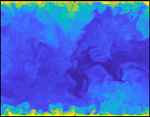
Figure 4 shows the instantaneous streamwise velocity and temperature at a constant  $x$ location in the cases M1R30A, M3R50A and M6R25A. The flow is very well mixed, with high-speed fluid intrusions from the top wall to the bottom wall, and vice versa. A pair of large-scale vortices is found in both the
  $u$ and
  $T$ fields in all three cases (Lozano-Durán & Jiménez Reference Lozano-Durán and Jiménez2014), leading to a high-momentum pathway and a low-momentum pathway across the spanwise direction. Again, while a small domain is less of a concern for low-order statistics, streamwise rollers that arise in Couette flow are not resolved, and we see high- and low-momentum pathways spanning the entire streamwise domain (Lee & Moser Reference Lee and Moser2018). M6R25A is at a lower Reynolds number than M1R30A and M3R50A, and the flow lacks fine-scale eddies. A higher Mach number leads to a larger variation of the fluid temperature in the flow field: the variation is about a few per cent of
  $T_b$ in the case M1R30A, and a few times
  $T_b$ in the case M6R25A.

Figure 4. Instantaneous streamwise velocity at a constant  $x$ location in (a) M1R30A, (b) M3R50A, and (c) M6R25A. Instantaneous temperature at a constant location in (d) M1R30A, (e) M3R50A, and (f) M6R25A. Here,
  $U_w$ is the wall velocity, and
  $T_b$ is the bulk temperature. For visualization purposes, the colour bar ranges in (d–f) are different.
Figure 5 shows the contours of the instantaneous wall-shear stress and wall temperature in the cases M1R30A, M3R50A and M6R25A. Footprints of the high- and low-momentum pathways are clearly visible in both the wall-shear stress and the wall temperature. Coherence in the streamwise direction, manifested as streaks, is found in the two lower Mach number cases, i.e. M1R30A and M3R50A (Yao & Hussain Reference Yao and Hussain2020). In the Mach 6 cases, we see spanwise coherence. The same is observed in Yu et al. (Reference Yu, Xu and Pirozzoli2019) and is a result of bouncing acoustic waves in the channel.

Figure 5. Instantaneous wall-shear stress in (a) M1R30A, (b) M3R50A, and (c) M6R25A. Instantaneous wall temperature in (d) M1R30A, (e) M3R50A, and (f) M6R25A.
4.2. Flow statistics
Figure 6 shows the Favre-averaged temperature, the mean density, the mean molecular viscosity and the semi-local-scaled wall-normal coordinate. The temperature decreases as a function of  $y$. Consequently, the density is an increasing function of
  $y$ (the mean pressure is approximately a constant in the channel), and the dynamic viscosity is a decreasing function of
  $y$. The increasing density and the decreasing viscosity together give rise to a
  $y^*$ such that
  $y^*>y^+$. The gradient of the temperature is zero at the wall because of the adiabatic condition, and similarly for the gradients of the density and the viscosity. Integrating the density profile
  $\bar {\rho }/\rho _b$ from the wall to the centre of the channel gives unity as a result of mass conservation. The Mach number strongly affects the statistics in figure 6. Higher Mach numbers lead to significant variations in temperature, density and viscosity across the channel.

Figure 6. Profiles of (a) temperature, (b) density, (c) dynamic viscosity, and (d) semi-local-scaled wall-normal distance. The insert in (a) shows the temperature profiles in the wall layer.
Figure 7 shows the mean velocity according to the Van Driest transformation (Van Driest Reference Van Driest1951) and the semi-local transformation (Patel et al. Reference Patel, Boersma and Pecnik2016). The data follow the linear scaling in the viscous sublayer in figures 7(a,b). Both the Van Driest transformation and the semi-local transformation collapse the adiabatic wall data in the logarithmic layer, but the transformed velocities are slightly above the incompressible logarithmic law of the wall. The upshift in the log layer has also been observed in the literature (Modesti & Pirozzoli Reference Modesti and Pirozzoli2016; Zhang et al. Reference Zhang, Duan and Choudhari2018; Yu et al. Reference Yu, Xu and Pirozzoli2019). A more in-depth discussion of the velocity falls outside the scope of this work.

Figure 7. Velocity profiles: (a) Van Driest transformed (Van Driest Reference Van Driest1951); (b) semi-local transformed (Patel et al. Reference Patel, Boersma and Pecnik2016). The two black lines are  $U=y$ and
  $U=\log (y)/\kappa +B$ (with proper normalization).
Figures 8(a–c) show the root-mean-square (r.m.s.) of the streamwise, wall-normal and spanwise velocity fluctuations. The streamwise velocity fluctuation is by far the most energetic component. The Couette flow configuration is known to give rise to a more energetic inner peak than the channel configuration (Pirozzoli, Bernardini & Orlandi Reference Pirozzoli, Bernardini and Orlandi2014). This explains an energetic inner peak in figure 8(a). A plateau develops in  $u''_{rms}$ at the (comparably) high Reynolds number cases above the buffer layer. A logarithmic layer could not yet be found in the profiles (
 $u^2$ is not shown) because of the limited Reynolds number. In addition to a more energetic inner peak, the Couette flow configuration is also known to give rise to a peak in
  $v_{rms}''$ at the centreline, which is also borne out in figure 8(b). Figure 8(d) shows the temperature r.m.s. We know from figure 6(a) that a large Mach number gives rise to a large temperature variation across the flow field, which, because of turbulence mixing, in turn leads a large temperature r.m.s.

Figure 8. Turbulent flow statistics: (a) r.m.s. of the streamwise velocity fluctuation; (b) r.m.s. of the wall-normal velocity fluctuation; (c) r.m.s. of the spanwise velocity fluctuation; (d) r.m.s. of the temperature fluctuation.
4.3. Temperature scaling
In this subsection, we compare the two scalings in (2.1) and (2.2) to DNS. We keep in mind that the original Van Driest temperature scaling and the original semi-local temperature scaling are singular for flows above adiabatic walls, and a data comparison with regard to those original scalings is not possible in this case.
Figure 9(a) shows the temperature profiles transformed according to the corrected Van Driest transformation in (2.1). We have the following observations. First, the transformation in (2.1) is non-singular for adiabatic walls, and the transformed adiabatic wall data follow the expected linear scaling in the viscous sublayer. Second, the adiabatic wall data and the hot wall data follow the expected logarithmic scaling closely in the logarithmic layer. Third, accounting for the flux  $\bar {q}$ in the Van Driest transformation does not help collapse the cold wall data (Patel et al. Reference Patel, Boersma and Pecnik2017). A direct conclusion of Van Driest transformation is the universality of
  $k_t$ as a function the viscous-scaled wall-normal coordinate
  $y^+$. Figure 9(b) shows the eddy conductivity as a function of the viscous-scaled wall-normal distance. We see that the adiabatic and hot wall data collapse and follow the scaling
  $\kappa _T y^+$ in the logarithmic layer, whereas the cold wall data fall below, which is consistent with the results in figure 9(a).

Figure 9. (a) Temperature profiles transformed according to the corrected Van Driest transformation (2.1). (b) The eddy conductivity.
Figure 10(a) shows the temperature profiles transformed according to the corrected semi-local scaling in (2.2), and figure 10(b) shows the eddy conductivity as a function of the semi-local-scaled wall-normal coordinate  $y^*$. It is seen from figure 10(a) that except for the case M6R25A, which is at an exceptionally low Reynolds number
  $Re_\tau =105$, all data follow the expected scaling in (2.4). Specifically, the transformed temperature profiles follow the linear scaling
  $Pr_w y^*$ in the viscous sublayer irrespective of whether the wall is adiabatic or isothermal, hot or cold. A clear log layer emerges and extends as the Reynolds number increases. Furthermore, we observe in figure 10(b) the universality of the eddy conductivity as a function of the semi-local-scaled wall-normal distance.

So far, we have relied on DNS to compute  $\bar {q}$ exactly. In the following, we test (2.40) and (2.41), where the term
  $\bar {q}$ is modelled according to (2.39). Figure 11 shows the transformed temperature profiles. We see that the transformed temperature profiles also follow the incompressible logarithmic law, although not as closely as in figures 9(a) and 10(a), suggesting that (2.39) is a good model for
  $\bar {q}$.


Finally, we compare DNS to the Walz equation in figure 12 to complete the story. For the DNS in table 1, the temperature at the channel centreline is lower than that at the wall, and  $\tilde {T}/\tilde {T}_c$ is a decreasing function of the velocity
  $\tilde {u}/\tilde {u}_c$. By adjusting the recovery constant, the Walz equation is able to match the DNS data very well, as illustrated in figure 12.

Figure 12. DNS (lines) and (1.7) (symbols). The recovery factor is set to  $r=0.89$. The frame of reference is such that the velocity is 0 at the wall.
5. Conclusions
Conventional temperature scalings are not applicable to high-speed turbulent flows with adiabatic walls because the wall heat flux is zero and the corresponding transformations become singular. By accounting for a specific diffusive flux of the kinetic energy ( $\bar {q}$) in the Van Driest (temperature) transformation and the semi-local (temperature) transformation, we show that
  $\theta _{\tau,c}^*\sim \bar {q}_w+\bar {q}$, i.e. a scale that is proportional to the local heat flux, is an appropriate temperature scale. The corrected transformations are
 \begin{equation} \theta_{vd,c}=\int_{0}^{\theta}\frac{{\rm d}{\theta}}{\theta_{\tau,c}^*} \end{equation}
and
 \begin{equation} {\theta}_{sl,c} = \int_0^{\theta}\left[1+\frac{y}{Re_\tau^*}\, \frac{{\rm d} Re_\tau^*}{{\rm d}y}\right]\frac{{\rm d}{\theta}}{\theta_{\tau,c}^*}, \end{equation}
where  $\theta =\tilde {T}_w-\tilde {T}$ is the temperature,
  $\theta _{\tau,c}^*= ({\bar {q}_w+\bar {q}})/{\bar {\rho } c_p u_\tau ^*}$,
  $\bar {q}= \overline {\sigma _{i2}}\overline {u_i}+\overline {\sigma _{i2}' u_i'}$
  $- \overline {\rho v'' u_i''}\,\tilde {u}_i- \overline {\rho v''\frac {1}{2} u_i'' u_i''}$,
  $\sigma _{ij}$ is the viscous stress tensor, and the superscript
  $*$ denotes normalization by local quantities. We show mathematically that the above corrected Van Driest and semi-local transformed temperatures follow
  $Pr_w y^+$ and
  $Pr_w y^*$, respectively, at the wall, irrespective of whether the wall is adiabatic or isothermal, hot or cold. The data favour the semi-local scaling in the logarithmic layer. The corrected semi-local temperature scaling is able to collapse the adiabatic, hot and cold wall data, but the Van Driest scaling is able to collapse the adiabatic and hot wall data only. In addition, we also show that the Walz equation is consistent with both the Van Driest transformation and the semi-local transformation, thereby unifying all existing theories.
This work patches the existing temperature scalings so that they can handle both adiabatic and non-adiabatic walls. The general framework in Morkovin (Reference Morkovin1962) remains intact, and we assume a simple viscous layer plus logarithmic layer structure. This assumption has recently been shown to be imprecise, particularly when one considers dissipation (Wei et al. Reference Wei, Fife, Klewicki and McMurtry2005a,Reference Wei, Fife, Klewicki and McMurtryb; Zhou, Pirozzoli & Klewicki Reference Zhou, Pirozzoli and Klewicki2017). Relaxing the above assumption would break the general framework in Morkovin (Reference Morkovin1962) and may give rise to more accurate scalings, but that is left for future investigation.
Funding
Y.S. acknowledges financial support from NSFC 91752202. Y.L. acknowledges the startup support from the Chinese Academy of Sciences.
Declaration of interests
The authors report no conflict of interest.


