1. Introduction
Turbulent thermal convection characterises many physical phenomena such as heat transport in stars (Busse Reference Busse1970), atmospheric flows (Wyngaard Reference Wyngaard1992) and oceanic currents (Thorpe Reference Thorpe2004). Even though these phenomena appear to be very different from one another, they share some fundamental features and can therefore be studied by using essentially the same set of equations (Busse Reference Busse1978). The most commonly studied configuration resembling these flows is Rayleigh–Bénard convection, i.e. a fluid layer that is heated from below and cooled from above. This simple configuration helped to shed some light on the rich physics of turbulent thermal convection, both in terms of the large-scale (Ahlers, Grossmann & Lohse Reference Ahlers, Grossmann and Lohse2009) and small-scale (Lohse & Xia Reference Lohse and Xia2010) dynamics. Several studies enriched the classical Rayleigh–Bénard system with additional features such as emulsions (Liu et al. Reference Liu, Chong, Ng, Verzicco and Lohse2021a), two fluid layers (Liu et al. Reference Liu, Chong, Wang, Ng, Verzicco and Lohse2021b), phase transition (Wang, Mathai & Sun Reference Wang, Mathai and Sun2019) and point-like particles (Oresta & Prosperetti Reference Oresta and Prosperetti2013). To the best of the authors’ knowledge, there has been no previous study considering suspensions of finite-size particles (or non-colloidal suspensions) under turbulent conditions. Given the importance of particle-laden natural convection in applications such as atmospheric pollution (Xu et al. Reference Xu, Tao, Shi and Xi2020) and energy harvesting in solar thermal plants (Pouransari & Mani Reference Pouransari and Mani2017; Rahmani et al. Reference Rahmani, Geraci, Iaccarino and Mani2018), the present study focuses on turbulent Rayleigh–Bénard convection in non-colloidal suspensions.
Two of the most important characteristics of turbulent Rayleigh–Bénard convection are the large-scale circulation structures and the boundary layers that form next to the horizontal, thermally active walls. The large-scale circulation structures are fed by plumes ejected from the boundary layers, and their behaviour is strongly affected by the domain geometry (Zhou, Sun & Xia Reference Zhou, Sun and Xia2007). These structures can exhibit oscillations of the circulation plane (Castaing et al. Reference Castaing, Gunaratne, Heslot, Kadanoff, Libchaber, Thomae, Wu, Zaleski and Zanetti1989) and azimuthal rotations (Brown & Ahlers Reference Brown and Ahlers2006) in cylindrical geometries, in addition to random cessations and reversals in cylindrical (Xi & Xia Reference Xi and Xia2007) or rectangular (Sugiyama et al. Reference Sugiyama, Ni, Stevens, Chan, Zhou, Xi, Sun, Grossmann, Xia and Lohse2010) domains. The structure of the large-scale circulation is significantly different in two-dimensional and three-dimensional simulations, both in terms of shape and velocity distribution (Demou & Grigoriadis Reference Demou and Grigoriadis2019), making three-dimensional simulations necessary for the accurate representation of these structures. As concerns the second aspect, the study of the boundary layers in Rayleigh–Bénard convection is of great importance because thermal convection theories and models rely on assumptions on the boundary layer dynamics (e.g. Grossmann & Lohse Reference Grossmann and Lohse2000; Ahlers et al. Reference Ahlers, Brown, Araujo, Funfschilling, Grossmann and Lohse2006), and this small region features the largest temperature gradients in contrast to the nearly isothermal bulk region. In detail, the near-wall distribution of temperature can be divided into: (i) the linear region, which is associated with the viscous sub-layer and in which thermal conduction accounts for most of the heat transfer, (ii) the transitional region, which accommodates the edge of the boundary layer and the maximum root-mean-square (r.m.s.) values of the temperature field and (iii) the bulk region, which features a nearly zero temperature gradient and is therefore dominated by thermal convection (Castaing et al. Reference Castaing, Gunaratne, Heslot, Kadanoff, Libchaber, Thomae, Wu, Zaleski and Zanetti1989; Wang & Xia Reference Wang and Xia2003; Zhou & Xia Reference Zhou and Xia2013). Both the structure of the large-scale circulation and the thickness of the boundary layers are expected to be significantly affected by the addition of a solid non-colloidal dispersed phase to the traditional Rayleigh–Bénard configuration.
Laminar Rayleigh–Bénard convection in non-colloidal suspensions was only recently studied by Kang, Yoshikawa & Mirbod (Reference Kang, Yoshikawa and Mirbod2021). More specifically, these authors focused on the effect of the particles on the transition from a conductive to a convective state using as the suspension continuum model the suspension balance model. Using linear stability analysis, it was shown that the critical Rayleigh number increases with increasing particle volume fraction, while the critical wavenumber of the instability remains the same. The mechanism responsible for the increase of the critical Rayleigh number is the dissipative force, which is intensified as the effective viscosity of suspensions increases. These authors also carried out numerical simulations of the convective regime and reported the decrease of the Nusselt number with increasing particle volume fraction, in line with the decay of the convective flow for higher volume fractions. Shear-induced particle migration was also observed, with the particles accumulating in the core of the large-scale circulation structures, away from the fast-moving periphery.
In the turbulent regime, Rayleigh–Bénard convection was studied in the presence of point-like particles which also can affect the flow (i.e. two-way coupling between fluid and particles), see Oresta & Prosperetti (Reference Oresta and Prosperetti2013) and Park, O'Keefe & Richter (Reference Park, O'Keefe and Richter2018). These studies demonstrated that the heat transfer and flow structures can be significantly affected by the particle properties, in particular particle diameter and inertia. Other studies considered turbulent thermal convection in the presence of point-like vapour bubbles, incorporating the effects of bubble volume change through condensation and evaporation (Oresta et al. Reference Oresta, Verzicco, Lohse and Prosperetti2009; Lakkaraju et al. Reference Lakkaraju, Schmidt, Oresta, Toschi, Verzicco, Lohse and Prosperetti2011, Reference Lakkaraju, Stevens, Oresta, Verzicco, Lohse and Prosperetti2013). Even though these studies provided useful insight into turbulent thermal convection in the presence of point-like particles, a comprehensive investigation is still missing for finite-size particles.
Turbulent heat transfer in suspensions of finite-size particles was mainly studied in forced convection. In the laminar regime, Metzger, Rahli & Yin (Reference Metzger, Rahli and Yin2013) studied the effects of shear-induced particle diffusion in Couette flows. They reported that the particle movement induces fluctuations in the fluid velocity, leading to heat transfer enhancement. Ardekani et al. (Reference Ardekani, Abouali, Picano and Brandt2018a) performed interface-resolved simulations, similar to this study, and showed that particle inertia further increases the heat transfer rate, especially for lower particle volume fractions. In a laminar pipe flow, Ardekani et al. (Reference Ardekani, Al Asmar, Picano and Brandt2018b) confirmed the heat transfer enhancement in the presence of particles and observed that larger particles produced higher heat transfer rates. The same study also considered turbulent conditions and reported that the particles have the opposite effect on the heat transfer rates, causing the laminarisation of the core region of the pipe even for relatively low particle volume fractions and thus a relative reduction of heat transfer. Yousefi et al. (Reference Yousefi, Ardekani, Picano and Brandt2021) studied turbulent channel flows, focusing on the characterisation of the different regimes of heat transfer encountered when varying the Reynolds number from laminar to turbulent conditions and particle volume fraction up to 35 %. Similarly to Ardekani et al. (Reference Ardekani, Al Asmar, Picano and Brandt2018b), the maximum heat flux rates reported by Yousefi et al. (Reference Yousefi, Ardekani, Picano and Brandt2021) were found at low particle volume fractions,  ${O}(10\,\%)$; the heat transfer, however, decreases below the single-phase turbulent values for higher volume fractions due to particle migration and the laminarisation of the flow in the channel core, see also Brandt & Coletti (Reference Brandt and Coletti2022).
This study aims to quantify the effects of dispersed finite-size particles in turbulent Rayleigh–Bénard convection. The suspended particles are neutrally buoyant, with all thermophysical properties matching the properties of the fluid. In particular, the focus is on revealing the modification of key heat-transfer-related quantities (Nusselt number and thermal boundary layer thickness), and on describing the underlying physical processes, driving these changes in the presence of particles. The remainder of this paper is structured as follows: § 2 presents the mathematical description of the physical problem and aspects of the numerical method used to solve the governing equations. The main results are shown and discussed in § 3. First, the parametric investigation of the particle volume fraction is presented in terms of flow visualisation (§ 3.1), heat transfer modulation (§ 3.2), two-phase statistics (§ 3.3), turbulent kinetic energy (TKE) budgets (§ 3.4), heat transfer budgets (§ 3.5) and two-point correlations (§ 3.6). Moreover, the parametric investigation of the particle size is presented in §3.7, utilising many of the statistical quantities mentioned above. Finally, § 4 concludes the study, listing the main findings.
2. Mathematical formulation and numerical method
2.1. Governing equations
Considering a Newtonian fluid within the limits of the Oberbeck–Boussinesq approximation (Oberbeck Reference Oberbeck1879; Boussinesq Reference Boussinesq1903), the governing equations for the incompressible fluid phase become
 $$\begin{gather} \boldsymbol{\nabla}\boldsymbol{\cdot} \boldsymbol{{u}_f}= 0, \end{gather}$$
 $$\begin{gather}\frac{\partial \boldsymbol{{u}_f}}{\partial {t}}+ \boldsymbol{{u}_f} \boldsymbol{\cdot} \boldsymbol{\nabla} \boldsymbol{{u}_f}={-}\frac{1}{{\rho}_f}\boldsymbol{\nabla} {P}+{\nu}_f \boldsymbol{\nabla}^2 \boldsymbol{{u}_f} + \left[1-{\beta}_f\left({T}_f-{T}_0\right)\right]\boldsymbol{{g}} + \boldsymbol{{f}}, \end{gather}$$
 $$\begin{gather}\frac{\partial {T}_f}{\partial {t}}+\boldsymbol{{u}_f} \boldsymbol{\cdot} \boldsymbol{\nabla} {T}_f = {\alpha}_f {\nabla}^2 {T}_f. \end{gather}$$
In the above equations,  $\boldsymbol {{u}_f}$ is the velocity vector of the fluid phase with individual components
  $({u}_f,{v}_f,{w}_f)$ along
  $({x},{y},{z})$,
  ${P}$ is the pressure and
  ${T}_f$ the fluid temperature. Moreover,
  ${\rho }_f$,
  ${\nu }_f$,
  ${\alpha }_f$ and
  ${\beta }_f$ denote the density, kinematic viscosity, thermal diffusivity and thermal expansion of the fluid. Furthermore,
  ${t}$ denotes time,
  $\boldsymbol {{g}}=-9.81\boldsymbol {\hat {z}}$ is the gravity vector and
  ${T}_0$ is a reference temperature inside the domain. The influence of particles on the fluid phase motion is introduced via the source term
  $\boldsymbol {{f}}$, which is activated in the vicinity of the particle surface to indirectly impose the no-slip and no-penetration boundary conditions at the moving solid boundary.
The rigid particles are considered to be spherical and neutrally buoyant (constant density, neglecting thermal expansion) with the same properties as the fluid phase. The Newton–Euler equations are used to describe the motion of the particles (linear and angular velocity), along with the heat transfer equation to calculate the temperature in the solid phase
 $$\begin{gather} m_p\frac{{\rm d} \boldsymbol{u}_p}{{\rm d} t}= \boldsymbol{f}_c + \oint_{\partial \varOmega_p} {\boldsymbol{\tau}} \boldsymbol{\cdot}\boldsymbol{n}_p\,{\rm d} A, \end{gather}$$
 $$\begin{gather}I_p\frac{{\rm d} \boldsymbol{\omega}_p}{{\rm d} t}= \boldsymbol{\tau}_c + \oint_{\partial \varOmega_p} \boldsymbol{r}\times\left( {\boldsymbol{\tau}} \boldsymbol{\cdot}\boldsymbol{n}_p\right){\rm d} A, \end{gather}$$
 $$\begin{gather}\frac{\partial T_p}{\partial t}+\boldsymbol{u}_p \boldsymbol{\cdot} \boldsymbol{\nabla} T_p = \alpha_p \nabla^2 T_p. \end{gather}$$
In these equations,  $\boldsymbol {u}_p$ and
  $\boldsymbol {\omega }_p$ denote the particle linear and angular velocity vectors, while
  $m_p$ and
  $I_p$ denote the particle mass and moment of inertia. Moreover
  $\boldsymbol {f}_c$ and
  $\boldsymbol{\tau}_c$ model the force and torque resulting from any short-range particle–particle and particle–wall interactions, and
  ${\boldsymbol{\tau}}$ is the fluid stress tensor. The surface integrals are calculated over the particle surface
  $\partial \varOmega _p$, with an outward-pointing normal vector
  $\boldsymbol {n}_p$ and a position vector
  $\boldsymbol {r}$ relative to the particle centre. The heat transfer inside the particles is governed by the same equation as the corresponding equation for the fluid, with
  $T_p$ and
  $\alpha _p$ denoting the temperature and thermal diffusivity of the particle phase.
2.2. Numerical method
We use the direct-forcing immersed boundary method (IBM), initially developed by Uhlmann (Reference Uhlmann2005) and modified by Breugem (Reference Breugem2012), to fully resolve the fluid–solid interactions. A volume of fluid (VoF) approach (Hirt & Nichols Reference Hirt and Nichols1981) is coupled to the IBM to solve the temperature equation in the two phases (Ström & Sasic Reference Ström and Sasic2013). The method has been used extensively with several validations reported by Picano, Breugem & Brandt (Reference Picano, Breugem and Brandt2015), Lashgari et al. (Reference Lashgari, Picano, Breugem and Brandt2016) and Ardekani et al. (Reference Ardekani, Costa, Breugem and Brandt2016) for the fluid–solid interactions and by Ardekani et al. (Reference Ardekani, Abouali, Picano and Brandt2018a,Reference Ardekani, Al Asmar, Picano and Brandtb) and Majlesara et al. (Reference Majlesara, Abouali, Kamali, Ardekani and Brandt2020) for the heat transfer in particle-laden flows. Furthermore, direct comparison of the numerical results with the experimental measurements of Zade (Reference Zade2019) at dense regimes verified the excellent accuracy of the numerical code. All the details of the implementation are presented in the aforementioned references. Nonetheless, for the sake of completeness, a brief description of the method is also presented here.
The Navier–Stokes equations governing the fluid phase dynamics are solved on a uniform  $(\Delta x = \Delta y = \Delta z)$ and staggered Cartesian grid. The spherical particles are discretised by a set of Lagrangian points, uniformly distributed along their surfaces. The IBM forcing scheme consists of three steps: (i) the fluid prediction velocity is interpolated from the Eulerian to the Lagrangian grid, (ii) the IBM force required for matching the local fluid velocity and the local particle velocity is computed on each Lagrangian grid point and (iii) the resulting IBM force is spread from the Lagrangian to the Eulerian grid. The interpolation and spreading operations are done through the regularised Dirac delta function of Roma, Peskin & Berger (Reference Roma, Peskin and Berger1999), which acts over three grid points in all coordinate directions.
Using the VoF approach, proposed in Ardekani et al. (Reference Ardekani, Abouali, Picano and Brandt2018a), the velocity of the combined phase is defined at each point in the domain as
 \begin{equation} \boldsymbol{u}_{cp} = \left( 1 - \xi \right) \boldsymbol{u}_f + \xi \boldsymbol{u}_p, \end{equation}
where  $\boldsymbol {u}_f$ is the fluid velocity and
  $\boldsymbol {u}_p$ the solid phase velocity, obtained as the rigid body motion of the particle at the desired point. In other words, the fictitious velocity of the fluid phase trapped inside the particles is replaced by the particle rigid body motion velocity when solving the temperature equation inside the solid phase; this velocity is computed as
  $\boldsymbol {u}_p + \boldsymbol {\omega }_p \times \boldsymbol {r}$ with
  $\boldsymbol {r}$, the position vector from the centre of the particle. The phase indicator
  $\xi$ is obtained from the exact location of the fluid/solid interface and used to distinguish the solid and the fluid phases within the computational domain. Also,
  $\xi$ is computed at the velocity (cell faces) and the pressure points (cell centre) throughout the staggered Eulerian grid. This value varies between
  $0$ and
  $1$ based on the solid volume fraction of a cell of size
  ${\Delta x}$ around the desired point, then
  $\boldsymbol {u}_{cp}$ is used to solve a unified temperature equation, which combines both (2.3) and (2.6). It should be noted that the computed
  $\boldsymbol {u}_{cp}$ remains a divergence free velocity field.
Accounting for the inertia and buoyancy forces of the fictitious fluid phase inside the particle volume and using the IBM, (2.4) and (2.5) are rewritten as
 $$\begin{gather} \rho_p \varOmega_p \frac{ \mathrm{d} \boldsymbol{u}_{p}}{\mathrm{d} t} \approx{-}\rho_f \sum_{l=1}^{N_L} \boldsymbol{f}_l \Delta \varOmega_l + \rho_f \frac{\mathrm{d}}{\mathrm{d} t} \left(\int_{\varOmega_p} \boldsymbol{u}\,\mathrm{d} \varOmega \right) - \int_{\varOmega_p} \rho_b \boldsymbol{g} \mathrm{d} \varOmega + \rho_p \varOmega_p \boldsymbol{g} +\boldsymbol{f}_c, \end{gather}$$
 $$\begin{gather}\boldsymbol{I}_p \frac{ \mathrm{d} \pmb{\omega}_{p} }{\mathrm{d} t} \approx{-}\rho_f \sum_{l=1}^{N_L} \boldsymbol{r}_l \times \boldsymbol{f}_l \Delta \varOmega_l + \rho_f \frac{ \mathrm{d}}{\mathrm{d} t} \left(\int_{\varOmega_p} \boldsymbol{r} \times \boldsymbol{u} \mathrm{d} \varOmega \right) - \int_{\varOmega_p} \boldsymbol{r} \times \rho_b \boldsymbol{g} \mathrm{d} \varOmega + \boldsymbol{\tau}_c, \end{gather}$$
where the first terms on the right-hand side describe the IBM force and torque as the summation of all the point forces  $\boldsymbol{f}_l$ on the surface of the particle. The second terms account for the inertia of the fictitious fluid phase trapped inside the particle and the third terms consider the correction due to applying the buoyancy force to the whole computational domain (including the fictitious fluid phase trapped inside the particle). Here,
  $\rho _b$ is the variable density of the fluid, assuming the Boussinesq approximation. Finally,
  $\boldsymbol {f}_c$ and
  $\boldsymbol {\tau}_c$ are the force and the torque exerted during the particle–particle/wall interactions. When the gap between two particles (or a particle and the wall) is smaller than the grid spacing, the IBM fails to resolve the short-range hydrodynamic interactions. Therefore, we use a lubrication correction model based on the asymptotic analytical expression for the normal lubrication force between two equal spheres (Brenner Reference Brenner1961). When the particles are in collision, the lubrication force is turned off and a collision force based on the soft-sphere model is activated. The restitution coefficients, used for normal and tangential collisions, are
  $0.97$ and
  $0.1$, with Coulomb friction coefficient
  $0.15$. More details on the short-range models and corresponding validations can be found in Costa et al. (Reference Costa, Boersma, Westerweel and Breugem2015).
2.3. Dimensionless parameters
Considering the type and properties of the particles discussed in the previous section, the physical problem studied here is characterised by the following dimensionless parameters:
(i) Rayleigh number,
 $Ra=|\boldsymbol {g}|\beta \Delta T L^3/(\nu \alpha )$;
(ii) Prandtl number,
$Pr = \nu /\alpha$;(iii) Particle volume fraction,
$\varPhi =n_p\varOmega _p/\varOmega _{tot}$;(iv) Stokes Number,
$St = \tau _p/\tau _f$.


In the above expressions,  $L$ is the reference length and
  $\Delta T = T_h-T_c$ is the temperature difference between the heated (
 $T_h$) and cooled (
 $T_c$) boundaries of the domain. Moreover,
  $n_p$ and
  $\varOmega _p$ denote the total number of particles and the volume of each particle. The Stokes number is defined as the ratio of the characteristic particle time scale
  $\tau _p=d_p^2/(18\nu )$, where
  $d_p$ is the particle diameter, to a characteristic fluid time scale
  $\tau _f$. Depending on the definition of
  $\tau _f$, two different Stokes number definitions can be given: (i)
  $St_{K}=d_p^2\epsilon ^{1/2}/(18\nu ^{3/2})$ based on the Kolmogorov time scale
  $(\nu /\epsilon )^{1/2}$, where
  $\epsilon$ is the energy dissipation rate, and (ii)
  $St_{f} = {d^*_p}^2 (\mathrm {Ra}/\mathrm {Pr})^{1/2}/18$, based on the free-fall time scale
  $(L/(g \beta \Delta T))^{1/2}$, where
  $d^*_p$ is the dimensionless particle diameter. Both of these definitions are important in characterising the flow since
  $St_{K}$ characterises the particle response to the effects of the smaller flow scales, while
  $St_{f}$ characterises the large-scale effects.
The most important output parameter is the Nusselt number, expressing the heat transfer inside the cavity and defined as  $Nu=h L / k$, where
  $h$ and
  $k$ denote the convection and conduction heat transfer coefficients. In the simulations, the Nusselt number over a surface
  $S$ with an outward-pointing normal vector
  $\boldsymbol {n}_S$ is calculated as,
  $Nu = \left \langle \boldsymbol {\nabla }T^* \boldsymbol {\cdot } \boldsymbol {n}_S\right \rangle _S$, where the operation
  $\left \langle \varPsi \right \rangle _{\psi }$ denotes the averaging of the dependent variable
  $\varPsi$ with respect to the independent variable
  $\psi$. Another informative output parameter is the Reynolds number
  $Re=LU/\nu$, which provides a measure of the extent of turbulence. More specifically, using the maximum r.m.s. of the fluid vertical velocity
  $w_f^{rms}$ as a characteristic velocity amplitude (as in Calzavarini et al. (Reference Calzavarini, Lohse, Toschi and Tripiccione2005) and van der Poel, Stevens & Lohse (Reference van der Poel, Stevens and Lohse2013) for example), the Reynolds number can be used to characterise the turbulence-inducing effect of the large-scale circulation structures that steer the flow.
The reference scales used for the non-dimensionalisation are  $L$ as the length scale,
  $(g \beta \Delta T L)^{1/2}$ as the velocity scale and the free-fall time scale. The temperature is made dimensionless as
  $T^*=(T-T_0)/(\Delta T)$, where
  $T_0=(T_h+T_c)/2$. To avoid overloaded notation, in the remainder of this paper all reported quantities are dimensionless without any special annotation.
2.4. Case description
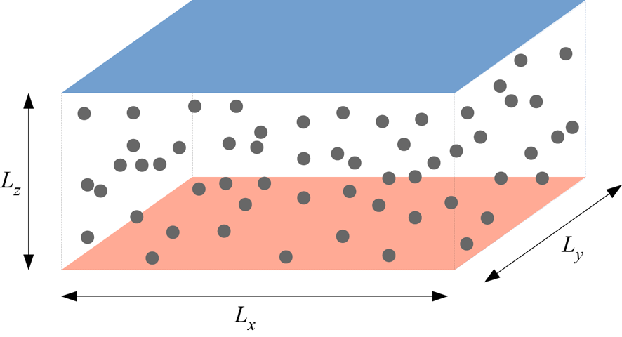
The three-dimensional geometry considered in the present study is shown in figure 1. A fluid layer containing the suspended particles is enclosed between two infinitely long horizontal solid walls, heated from below and cooled from above at a constant temperature. The  $x$ and
  $y$ directions are here assumed periodic. The domain dimensions are defined as
  $(L_x,L_y,L_z)=(2,2,1)$. The suspended spherical particles do not exhibit thermal expansion and are therefore considered neutrally buoyant. Moreover, all the particles have the same diameter and share the same thermophysical properties as the fluid. In §§ 3.1–3.6, a parametric study of the particle volume fraction is carried out, with
  $\varPhi =0\,\%\unicode{x2013}40\,\%$ and a fixed dimensionless particle diameter of
  $d^*_p=1/15$. Afterwards, in § 3.7, the effects of the particle size are explored, with
  $d^*_p=1/20\unicode{x2013}1/10$ and a fixed particle volume fraction of
  $\varPhi =35\,\%$. The values of the dimensionless parameters adopted along with other numerical parameters are shown in table 1, describing a total of 12 simulations. For simplicity we will use
  $d^*_p$ instead of
  $St_{f}$ to distinguish between the different cases. Moreover, since no analytical relation exists for calculating the energy dissipation rate as in single-phase convection (see e.g. Ahlers et al. Reference Ahlers, Grossmann and Lohse2009), an a posteriori analysis is required to calculate the Kolmogorov-based Stokes number, which is presented in §§ 3.4 and 3.7.

Figure 1. Schematic representation of the set-up used in the present study. The domain dimensions along the  $x$,
$x$,  $y$ and
  $z$ directions are
  $(L_x,L_y,L_z)=(2,2,1)$ and the diameter of the suspended particles is set to
  $d_p=1/15$. The fluid and the suspended particles are heated from the bottom wall (depicted in red) and cooled from the top wall (in blue).
Table 1. Physical and numerical parameters adopted in the present study. The free-fall-based Stokes number values corresponding to the dimensionless particle diameters listed are  $St_f=0.5$, 0.9 and 2.1 respectively. The values of the Kolmogorov-based Stokes number are presented in §§ 3.4 and 3.7. All cases were simulated using a Courant–Friedrichs–Lewy (CFL) condition value of 0.5.

To justify the adopted grid resolution, the criterion suggested in Shishkina et al. (Reference Shishkina, Stevens, Grossmann and Lohse2010) is used to calculate the maximum grid spacing  $\Delta z^{max}$ inside the thermal boundary layers. For the parameters used in the present study,
  $\Delta z^{max}=2^{-3/2}0.481^{-1}0.982^{-3/2}Nu^{-3/2}$. Considering a value
  $Nu=32.4$, calculated in the single-phase Rayleigh–Bénard convection (Stevens, Clercx & Lohse Reference Stevens, Clercx and Lohse2010; van der Poel et al. Reference van der Poel, Stevens and Lohse2013), this criterion gives
  $\Delta z^{max}=4.08\times 10^{-3}$, which corresponds to a uniform grid of 245 grid points along the wall-normal direction. Since the presence of the particles is expected to influence the flow, the present study adopted a uniform grid spacing which is almost half of what the criterion suggested, corresponding to
  $960 \times 960 \times 480$ grid cells. Relative to the particles, this resolution corresponds to 24, 32 and 48 grid points per particle diameter, for the different particle diameters listed in table 1. This resolution was proven to be appropriate in other turbulent direct numerical simulation studies (Ardekani et al. Reference Ardekani, Abouali, Picano and Brandt2018a; Yousefi, Ardekani & Brandt Reference Yousefi, Ardekani and Brandt2020; Yousefi et al. Reference Yousefi, Ardekani, Picano and Brandt2021).
All simulations are initialised using a statistically stationary solution from the single-phase case ( $\varPhi =0\,\%$), superimposed with the required number of particles at random locations. A dynamically adjusted time step is adopted, respecting the restriction of Wray's Runge–Kutta scheme (Wesseling Reference Wesseling2009) by using
  ${\rm CFL}=0.5$. The final time of each simulation was decided on an individual basis. More specifically, since the study will mainly present the statistics of the flow, an initial period is allowed for a statistically stationary state to be developed, followed by an extended time period to collect adequate statistical samples. This procedure is illustrated in figure 2(a), for the case with
  $\varPhi =20\,\%$ and
  $d^*_p=1/15$. After an initial transient, the Nusselt number on the bottom wall fluctuates around a distinct mean value. To avoid contaminating the statistical sample with the values at the initial stages of the simulation, the statistical sampling starts after the stabilisation of the mean Nusselt value. Figure 2(b) shows the running average of the Nusselt number on both the bottom and top walls, after the initial transient period. The statistical sample is considered large enough when the difference between the two time-averaged Nusselt values is of the order of
  $0.1\,\%$.
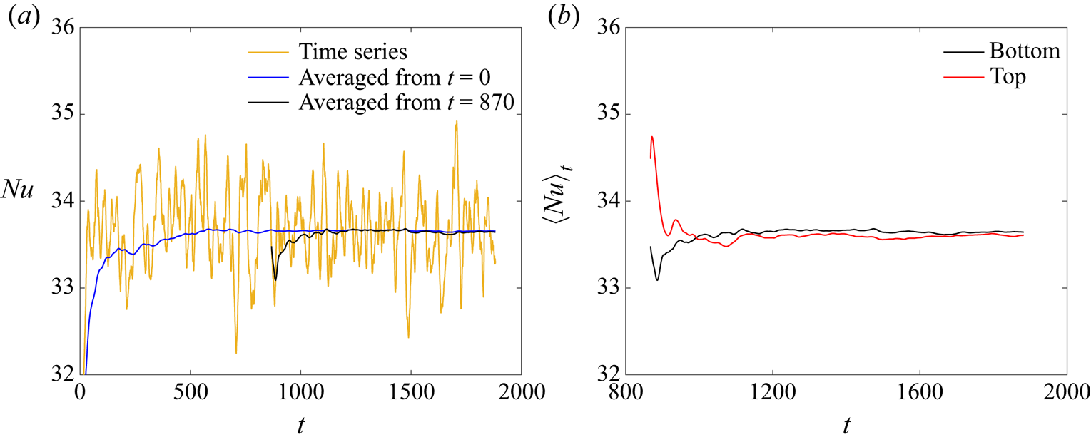
Figure 2. (a) Time series and running average of the Nusselt number on the bottom wall. (b) Running average of the Nusselt number on both the bottom and top walls. The plots correspond to the case  $\varPhi =20\,\%$ and
  $d^*_p=1/15$.
To further enhance the statistical samples, the top–bottom symmetry of the problem is exploited by averaging the fields between symmetric locations at the top and bottom halves of the cavity. Furthermore, since the  $x$ and
  $y$ directions are periodic, the statistical fields are also averaged along horizontal planes. The resulting time- and area-averaged observables (denoted as
  $\left \langle \,\cdot\, \right \rangle _{t,x,y}$ or simply
  $\left \langle \,\cdot\, \right \rangle$) vary only along the vertical direction
  $z$. The area-averaged r.m.s. values are calculated in a consistent manner, for example the r.m.s. values of the fluid temperature field are calculated as
 \begin{equation}
T_f^{rms}=\sqrt{\langle
T_f^2\rangle_{t,x,y}-\left\langle
T_f\right\rangle^2_{t,x,y}}.
\end{equation}
\begin{equation}
T_f^{rms}=\sqrt{\langle
T_f^2\rangle_{t,x,y}-\left\langle
T_f\right\rangle^2_{t,x,y}}.
\end{equation}
All the simulations presented in this study ran on 576 CPU processors. The single-phase simulation was performing on average 980 time steps per hour, while the simulation with the highest particle volume fraction  $\varPhi =40\,\%$ was performing 113 time steps per hour. Given that the time step was roughly the same in all cases, the simulation with
  $\varPhi =40\,\%$ was approximately 9 times slower than the single-phase simulation, highlighting the significant computational overhead of the particle calculations.
3. Results
3.1. Flow visualisation
To get a first appreciation of the flow within this configuration, figure 3 shows the instantaneous temperature fields and particle locations along a wall-normal  $y-z$ plane, for different values of the particle volume fractions and a fixed particle diameter of
  $d^*_p=1/15$. In all cases, hot and cold plumes are ejected from the bottom and top boundary layers. These plumes feed the large-scale circulation in the bulk of the cavity, which is evident from the particle motion. In particular, the bulk of the cavity accommodates regions with coordinated upward and downward particle motions. Furthermore, as better illustrated in figure 4, with increasing particle volume fraction there exists an increased layering of particles along the bottom and top walls. This is more pronounced for
  $\varPhi =40\,\%$ (figure 4d), where the walls are covered with tightly packed particles. In addition, for smaller particle volume fractions, the particles appear to be cooler next to the bottom heated wall. As the particle volume fraction increases, the particles have, on average, a higher temperature, suggesting a longer residence time in the near-wall region.

Figure 3. Snapshots of the temperature field along with the particle locations in a wall-normal  $y$–
$y$– $z$ plane. The particles are coloured based on their vertical velocity
  $w$; (a)
  $\varPhi =10\,\%$, (b)
  $\varPhi =20\,\%$, (c)
  $\varPhi =30\,\%$ and (d)
  $\varPhi =40\,\%$. In all the cases,
  $d^*_p=1/15$. Since the contour plane is partially transparent, the particles with centres located behind the plane appear to have a halo around them.
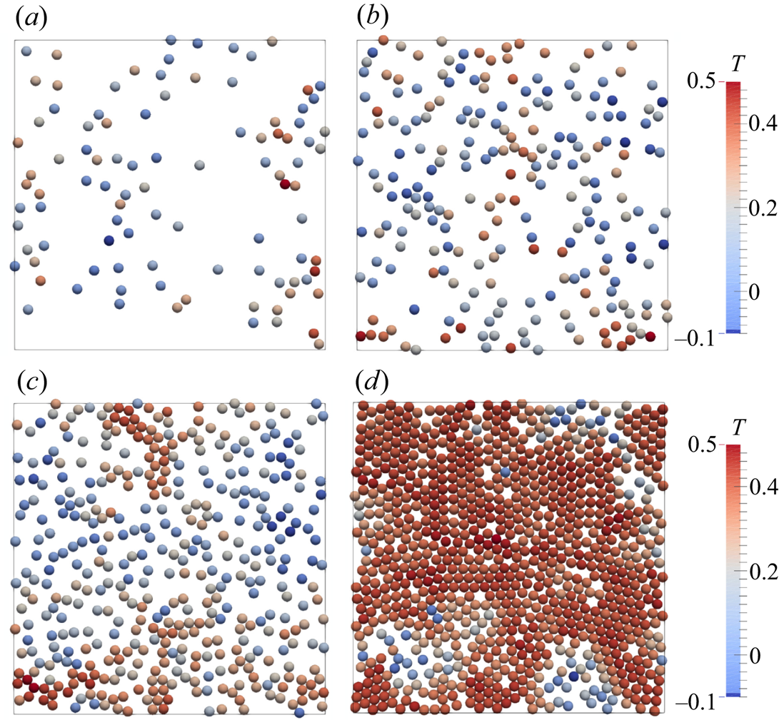
Figure 4. Snapshots of the first particle layer next to the bottom wall ( $x$–
$x$– $y$ plane). The particles are coloured based on their temperature; (a)
  $\varPhi =10\,\%$, (b)
  $\varPhi =20\,\%$, (c)
  $\varPhi =30\,\%$ and (d)
  $\varPhi =40\,\%$. In all the cases,
  $d^*_p=1/15$.
Focusing on the fluid phase, figure 5 shows two instantaneous temperature isosurfaces for different values of the particle volume fraction. These isosurfaces give a better understanding of the structure of the plumes that are ejected from the bottom and top boundary layers. Starting from  $\varPhi =10\,\%$, the bottom boundary layer features an active region with intense plume ejection next to a more quiescent region. The same is true for the top boundary layer, with its quiescent region located opposite the bottom boundary layer's active region, and vice versa. This three-dimensional plume configuration facilitates the presence of a large-scale circulation. For particle volume fractions up to 30 %, the presence of a solid phase intensifies the plumes in the quiescent regions. Furthermore, the particle inertia helps the plumes ejected from the active regions to travel through the bulk of the cavity all the way to the opposite boundary layer. By contrast, increasing the particle volume fraction even further, to 40 %, has the opposite effect; the ejection of plumes is suppressed, without a clear distinction between active and quiet regions and no clear indication of a large-scale circulation structure as we shall discuss in detail below.
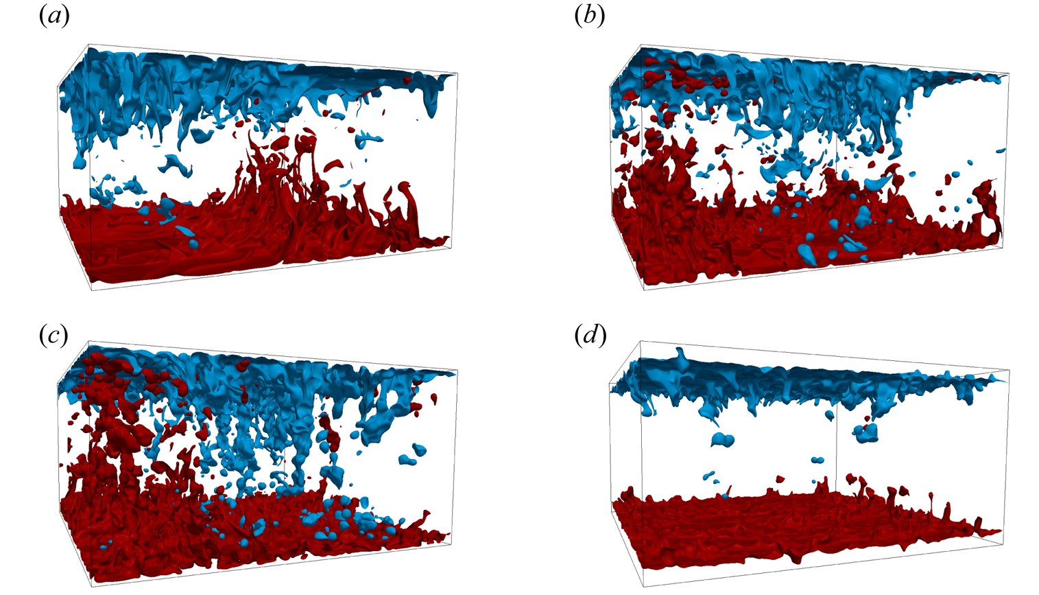
Figure 5. Snapshots of temperature isosurfaces for (a)  $\varPhi =10\,\%$, (b)
  $\varPhi =20\,\%$, (c)
  $\varPhi =30\,\%$ and (d)
  $\varPhi =40\,\%$. In all the cases,
  $d^*_p=1/15$. Red colour corresponds to
  $T=0.1$ and blue colour corresponds to
  $T=-0.1$.
3.2. Heat transfer modulation
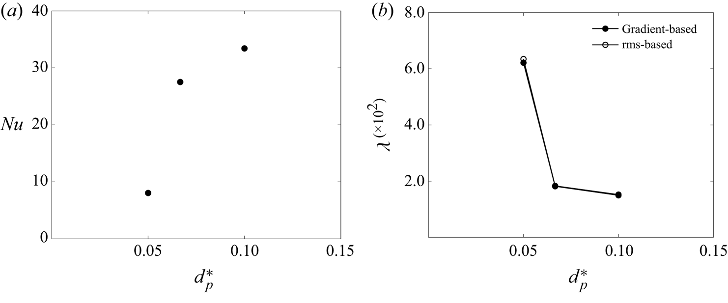
The heat transfer inside the cavity is expressed through the Nusselt number, defined in § 2.3, and shown in figure 6(a) as a function of the particle volume fraction, for  $d^*_p=1/15$. The Nusselt number is calculated by averaging the heat fluxes at the bottom and top walls. Up to
  $\varPhi =25\,\%$, the Nusselt number increases almost linearly with the particle volume fraction, reaching a maximum value of 33.8, from 31.8 at
  $\varPhi =0\,\%$; a relatively mild increase of approximately 6 %. Beyond that point, a steep decrease is observed with the Nusselt number dropping to 7.8 for the highest particle volume fraction considered,
  $\varPhi =40\,\%$. This observation is similar to what reported in Yousefi et al. (Reference Yousefi, Ardekani, Picano and Brandt2021) for finite-size particle suspensions in a channel flow. In that study, the maximum Nusselt number was encountered at a particle volume fraction of 10 %, for all the Reynolds numbers within the transitional or fully turbulent regimes. The authors attributed the decrease of the Nusselt number at higher values of
  $\varPhi$ to the decreased mixing due to the particle migration towards the channel core. More specifically, turbulence fluctuations decrease significantly at the centreline where the particles move together as a compact aggregate with reduced relative velocities and rotation rates. This is, however, different from what is observed in figure 3 for the present Rayleigh–Bénard case, where the particle layers next to the walls become more packed when increasing the particle volume fraction. This will be examined quantitatively in § 3.3, where the average local volume fraction inside the cavity is presented. In addition, to explain the effect of particle volume fraction on the heat transfer inside the cavity, the heat transfer budgets will be presented and discussed in § 3.5.
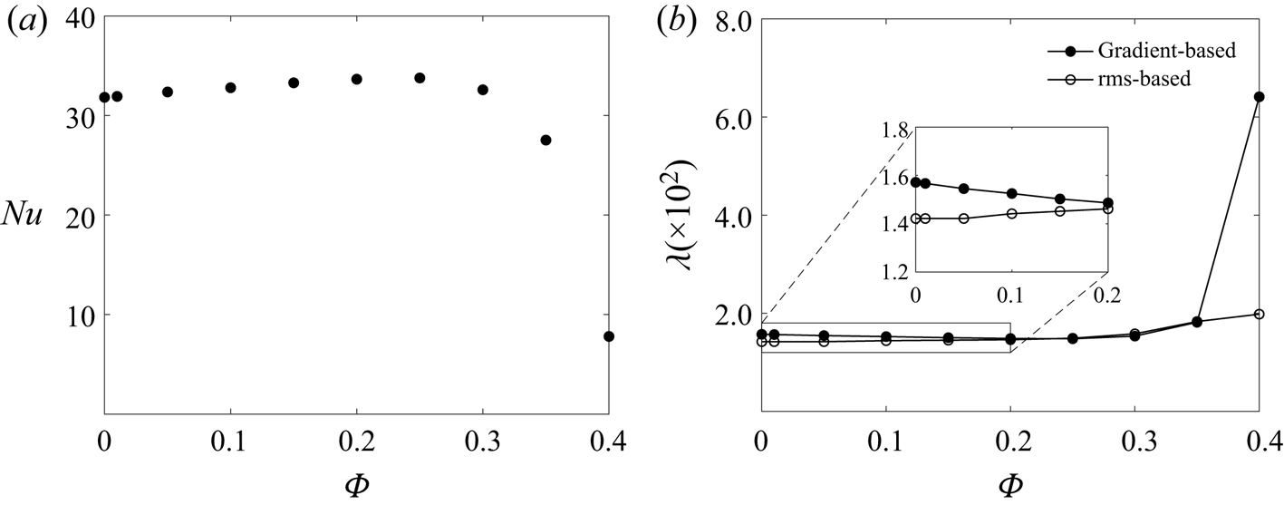
Figure 6. (a) Nusselt number and (b) thermal boundary layer thickness as a function of the particle volume fraction, for  $d^*_p=1/15$. The boundary layer thickness based on the gradient is defined in (3.1) and the r.m.s.-based definition given in (3.2). Both quantities are calculated by averaging the relevant quantities at the bottom and top walls.
Another important characteristic of thermal convection is the thermal boundary layer thickness, defined either using the temperature gradient at the wall
 \begin{equation}
\lambda^{\boldsymbol{\nabla} T} =
\frac{(\boldsymbol{\nabla}\langle T\rangle|_{z=0})^{{-}1}}{2},
\end{equation}
\begin{equation}
\lambda^{\boldsymbol{\nabla} T} =
\frac{(\boldsymbol{\nabla}\langle T\rangle|_{z=0})^{{-}1}}{2},
\end{equation}
or as the location of the maximum r.m.s. of the temperature field
 \begin{equation} \lambda^{rms} = \mathrm{argmax}_z (T^{rms}), \end{equation}
where  $T$ is the phase-averaged temperature. As shown in different single-phase studies (Wang & Xia Reference Wang and Xia2003; Demou & Grigoriadis Reference Demou and Grigoriadis2019), the two definitions do not necessarily coincide, with
  $\lambda ^{\boldsymbol {\nabla } T}$ calculated at the wall (therefore being closely associated with the Nusselt number), while
  $\lambda ^{rms}$ is calculated inside the flow. As a natural length scale,
  $\lambda ^{rms}$ was shown to be more effective in the scaling of higher-order moments of the temperature field (Tilgner, Belmonte & Libchaber Reference Tilgner, Belmonte and Libchaber1993; Zhou & Xia Reference Zhou and Xia2013). The values of the thermal boundary layer thickness obtained from both definitions are shown in figure 6(b) as a function of the particle volume fractions. As expected from its definition,
  $\lambda ^{\boldsymbol {\nabla } T}$ follows the opposite trend as of the Nusselt number, with a small decrease for moderate particle volume fractions and a steep increase beyond
  $\varPhi =25\,\%$. On the other hand,
  $\lambda ^{rms}$ increases monotonically with the solid volume fraction in the range explored. Starting from slightly different values at
  $\varPhi = 0\,\%$, the two definitions converge to approximately the same value at
  $\varPhi \approx 20\,\%$ and retain their agreement for up to
  $\varPhi \approx 35\,\%$. At the highest volume fraction considered, a large deviation is observed. Even though the temperature gradient at the walls decreases and
  $\lambda ^{\boldsymbol {\nabla } T}$ increases significantly, the maximum temperature r.m.s. value does not shift further from the walls, which explains the difference between the two values at the highest particle volume fractions. As observed in figure 3(d), the dense particle layer next to the walls enhances the mixing in the near-wall regions, therefore reducing the Nusselt number, yet it still induces significant thermal agitation in this region. These observations will be further substantiated by the investigation of the statistics of the temperature fields in § 3.3.2.
3.3. Two-phase statistics
3.3.1. Particle distribution
Of special interest is the local particle volume fraction  $\varphi$, defined as the fraction of a grid cell inside a particle. This observable serves as an indicator function, taking the value
  $\varphi =1$ when the grid cell is fully immersed in a particle and
  $\varphi =0$ when there is no solid phase inside the grid cell. Its time average is therefore the probability of finding the solid phase in the volume under investigation. With the present definition, the local volume fraction goes to zero as
  $z \to 0$ because there can only be contact in isolated points between the spheres and the solid boundary. Further exploiting the symmetries of our configuration, we will therefore consider the time- and area-averaged local particle volume fraction
  $\left \langle \varphi \right \rangle$ as a function of the vertical direction
  $z$, shown in figure 7 for the different values of the nominal particle volume fraction under investigation, and
  $d^*_p=1/15$. In all the cases, we see a peak close to the wall, indicating the presence of a layer of particles adjacent to the boundary, while the bulk of the cavity features a homogeneous local volume fraction distribution with
  $\left \langle \varphi \right \rangle \approx \varPhi$. A similar behaviour was also observed for moderate particle volume fractions in strongly turbulent channel flows, attributed to the one-sided wall–particle interactions (Costa et al. Reference Costa, Picano, Brandt and Breugem2016; Lashgari et al. Reference Lashgari, Picano, Breugem and Brandt2016; Yousefi et al. Reference Yousefi, Ardekani, Picano and Brandt2021). On the other hand, suspensions in laminar Rayleigh–Bénard convection exhibited the opposite behaviour of shear-induced particle migration to the core of the cavity (Kang et al. Reference Kang, Yoshikawa and Mirbod2021). The peak close to the wall is more pronounced as the particle volume fraction increases, confirming the increased layering of particles next to the walls depicted in the instantaneous fields shown in figure 3. In the present study, the average local volume fraction for the case with
  $\varPhi =40\,\%$ reaches a maximum value of
  $\varphi _{max}=0.832$. Given that the volume fraction for maximum circle packing is
  $0.907$ (Chang & Wang Reference Chang and Wang2010), the case with
  $\varPhi =40\,\%$ exhibits an almost fully packed particle layer next to the walls. A particle wall layer was first observed by Picano et al. (Reference Picano, Breugem and Brandt2015) in turbulent channel flow of dense suspensions, where the authors explained this formation by a mechanism similar to that usually observed in laminar Poiseuille and Couette flows (Yeo & Maxey Reference Yeo and Maxey2010, Reference Yeo and Maxey2011; Picano et al. Reference Picano, Breugem, Mitra and Brandt2013). Within this mechanism, once a particle reaches the wall, the strong wall–particle lubrication interaction stabilises the particle wall-normal position. Hence, it becomes difficult for the particles belonging to the first layer to escape from it.

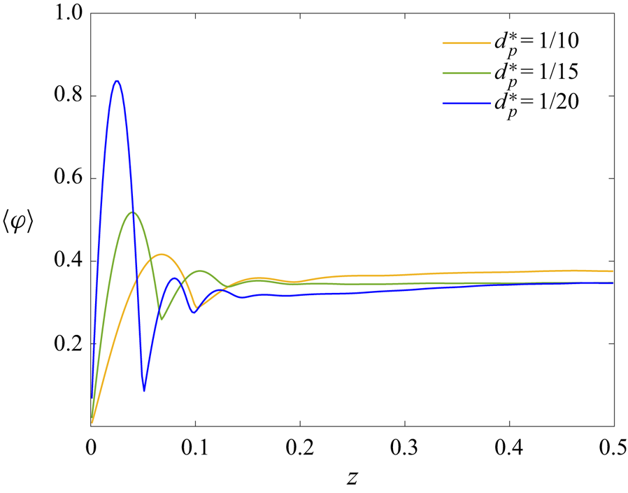
Figure 7. Average local particle volume fraction as a function of the vertical direction for different values of the particle volume fraction specified in this study. In all the cases,  $d^*_p=1/15$.
We also note that, as the particle volume fraction increases, the location of the maximum local volume fraction is also affected, moving closer to the wall by adding more particles. More specifically, at  $\varPhi =10\,\%$ the maximum is located at
  $z=0.051$, while at
  $\varPhi =40\,\%$ the maximum is at
  $z=0.034$, approximately half of the particle diameter from the wall. Consequently, the particles that form the dense layer at
  $\varPhi =40\,\%$ are in close proximity with the wall. In addition, as the particle volume fraction increases, a second and third maximum appear. Again, this second maximum further from the wall is more pronounced as the value of
  $\varPhi$ increases, but its location remains constant at
  $z=0.105$ (approximately one and a half particle diameters from the wall). These observations suggest that, as the particle volume fraction increases, the flow conditions lead to the formation of a second (less dense) particle layer in the vicinity of the wall. The case with
  $\varPhi =40\,\%$ also exhibits two additional smaller maxima, before the profile of the local volume fraction reaches a homogeneous distribution in the bulk of the cavity. In other words, by adding more particles to the flow, more layers are formed before the uniform distribution in the central region of the cavity is reached.
3.3.2. Temperature statistics
Figure 8 shows the wall-normal profiles of the temperature statistics for  $d^*_p=1/15$ and different particle volume fraction. Focusing first on the fluid and particle mean temperatures in figures 8(a) and 8(c), we note that the different profiles are similar in the different cases up to
  $\varPhi =30\,\%$, with a strong gradient next to the wall and almost isothermal conditions in the cavity core. These characteristics are also encountered in single-phase turbulent Rayleigh–Bénard studies (Zhou & Xia Reference Zhou and Xia2013; Demou & Grigoriadis Reference Demou and Grigoriadis2019). As the particle volume fraction increases, there is an increase of the temperature next to the heated wall (decrease next to the cooled wall) in the region around
  $z=0.05$ for both the fluid and the particles, in correspondence with the edge of the particle wall layer, before
  $T$ decays and reaches to the isothermal condition in the central region of the cavity. For
  $\varPhi =40\,\%$, this effect is much more pronounced and extends over a larger region, approximately up to two particle diameters from the wall. These results indicate a mixing enhancement in the vicinity of the wall, which is correlated with the accumulation of particles in this region, as discussed previously in relation to the volume fraction distributions in figure 7. Comparing the results pertaining the two phases, we note that the temperatures of the fluid and particles agree fairly well throughout the cavity, except for a small region between one and two particle diameters from the wall, where the temperature of the particles next to the heated (cooled wall) drops below (rises above) the fluid temperature.

Figure 8. Wall-normal profiles of the temperature statistics for different values of the particle volume fraction. (a) Mean fluid temperature, (b) r.m.s. of the fluid temperature, (c) average particle temperature and (d) r.m.s. values of the particle temperature. In all the cases,  $d^*_p=1/15$.
The intensity of the temperature fluctuations is shown in figures 8(b) and 8(d) for the fluid and particles. The profiles are characterised by a sharp increase with a maximum in the near-wall region, before decreasing towards the cavity core. Again, this behaviour is not very different to what has been reported in single-phase Rayleigh–Bénard studies (du Puits et al. Reference du Puits, Resagk, Tilgner, Busse and Thess2007; Zhou & Xia Reference Zhou and Xia2013). As the particle volume fraction increases up to 30 %, both the fluid and particle profiles exhibit increased r.m.s. values, revealing an increased thermal agitation throughout the cavity. In line with the variation of  $\lambda ^{rms}$ in figure 6, the location of the maximum r.m.s. value shifts slightly away from the wall when increasing the value of the volume fraction
  $\varPhi$. At
  $\varPhi =40\,\%$, the temperature fluctuation profiles are significantly altered, exhibiting decreased values and pronounced differences between fluid and particles. A secondary maximum appears in the fluid profile, at approximately one particle diameter from the global maximum. At this location, the particle temperature r.m.s. exhibits a spike that is even larger than the maximum closer to the wall. Similar temperature r.m.s. profiles were reported by Ciliberto & Laroche (Reference Ciliberto and Laroche1999) who studied thermal convection in the presence of roughness and observed that a second r.m.s. maximum appears when the thermal boundary layer is thin enough to interact with the heated plate roughness. This happens when the thermal boundary layer thickness is less than half of the roughness thickness (diameter of the largest spheres that were glued together to create the rough surfaces in the experiments). In the present study, the opposite effect is observed: the r.m.s. profiles exhibit a single r.m.s. maximum for the cases where the thermal boundary layer thickness is smaller than half the particle diameter (cases with
  $\varPhi <35\,\%$), while a secondary r.m.s. maximum is observed for the case where the thermal boundary layer thickness becomes comparable to the particle diameter (case with
  $\varPhi =40\,\%$). Therefore, even though the temperature r.m.s. profiles presented here exhibit similarities to thermal convection in the presence of roughness, the mechanisms that cause these effects are probably different. In the present study, these new r.m.s. maxima at
  $\varPhi =40\,\%$ are found between the maximum local volume fractions shown in figure 7, suggesting the increased influence of the particle motion for the thermal agitation in this region. To support this claim, the following section presents the fluid and particle velocity statistics.
3.3.3. Velocity statistics
The presence of counter-rotating large-scale circulation structures in the Rayleigh–Bénard configuration complicates the study of the area- and time-averaged velocity field, which reduces to almost zero after adequate sampling, i.e.  $\left \langle u\right \rangle = \left \langle v\right \rangle = \left \langle w\right \rangle =0$. Because of this, the velocity r.m.s. values reduce to
  $u^{rms}=\sqrt {\left \langle u^2\right \rangle }$,
  $v^{rms}=\sqrt {\left \langle v^2\right \rangle }$ and
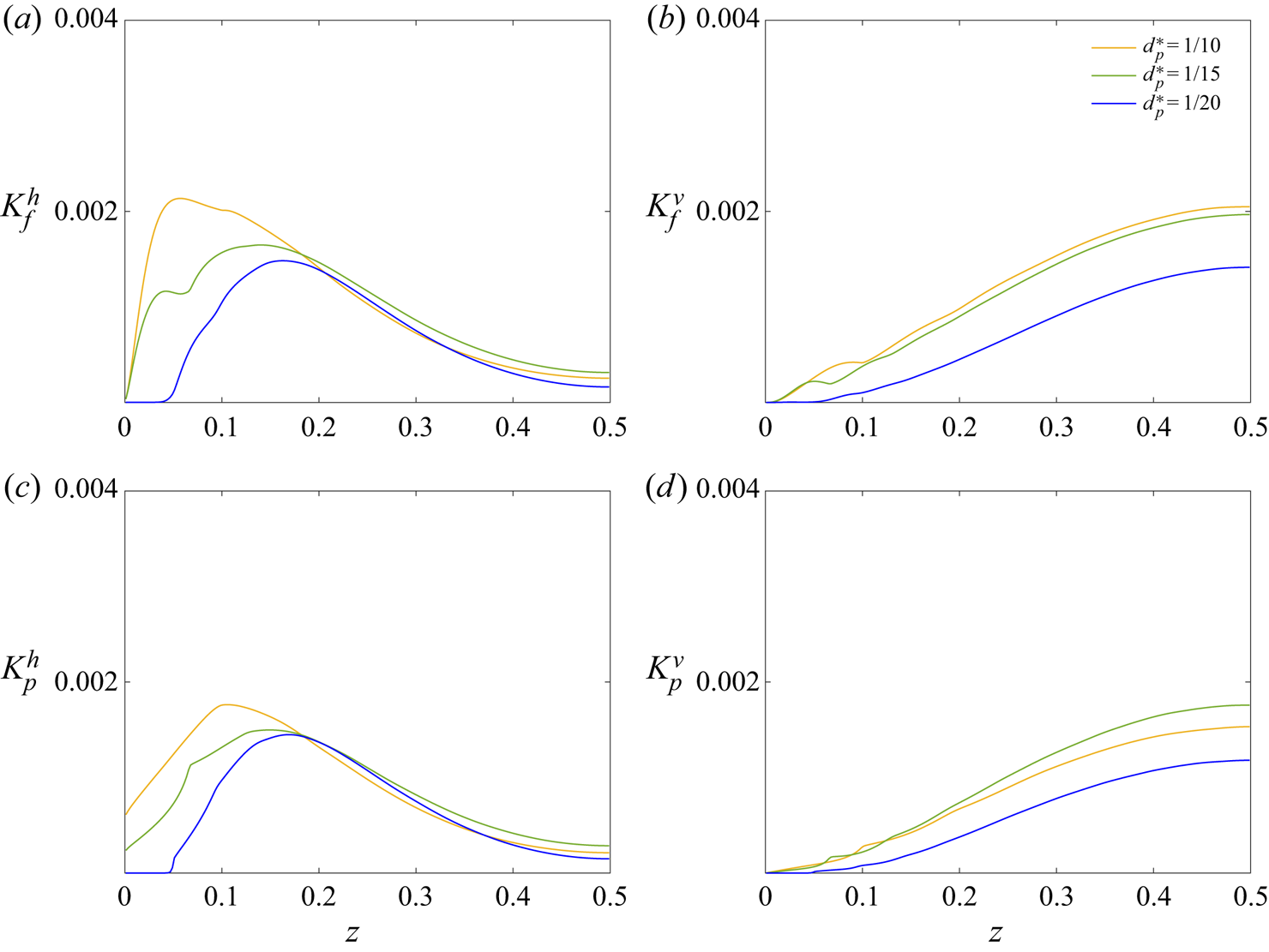
  $w^{rms}=\sqrt {\left \langle w^2\right \rangle }$. To identify the role of different flow structures, the average fluid and particle kinetic energy per unit mass can be divided into
 $$\begin{gather} K_f^h= \tfrac{1}{2}\left(\left( u_f^{rms}\right)^2+\left( v_f^{rms}\right)^2\right),\quad K_f^v = \tfrac{1}{2}\left( w_f^{rms}\right)^2, \end{gather}$$
 $$\begin{gather}K_p^h = \tfrac{1}{2}\left(\left( u_p^{rms}\right)^2+\left( v_p^{rms}\right)^2\right),\quad K_p^v = \tfrac{1}{2}\left( w_p^{rms}\right)^2, \end{gather}$$
where subscripts  $h$ and
  $v$ correspond to the horizontal and vertical contributions. The average kinetic energy can be used to characterise the flow large-scale motions. In particular, the horizontal contributions are associated with the velocity of the structures that sweep the boundary layers, while the vertical contributions are associated with the velocities in the bulk of the cavity.
The horizontal contributions of the fluid and particle average kinetic energy per unit mass are shown in figures 9(a) and 9(c), with  $d^*_p=1/15$. Similar to the temperature r.m.s. fields, the horizontal kinetic energy contributions reach a maximum at some distance from the wall and decay towards the bulk of the cavity. The big difference from the temperature r.m.s. fields is that increased particle volume fraction leads to decreased kinetic energy. Additionally, the variations with the particle volume fraction are larger for the kinetic energy than for the temperature fluctuations, even for moderate particle volume fractions. Nonetheless, similar to the temperature fluctuations, the location of the maximum moves away from the wall when increasing the value of
  $\varPhi$. This suggests a change in the way the large-scale circulation structures sweep the boundary layers. Otherwise known as ‘wind of turbulence’, these circulation structures unsettle the fluid in the vicinity of the wall and contribute to the development of the viscous boundary layers. The maximum value of the horizontal kinetic energy gives an indication of the location of the outer edge of the viscous boundary layer, as well as the location of the periphery of the large-scale circulation structures. In this context, the results for the horizontal kinetic energy distributions,
  $K^h_f$ and
  $K^h_p$, indicate the thickening of the viscous boundary layer, as well as the weakening of the rotation of the large-scale circulation structures with increasing particle volume fraction. Comparing the locations of the maximum of the kinetic energy and the temperature r.m.s., it is clear that the viscous boundary layer is much thicker than the thermal boundary layer, as expected from the value of the Prandtl number
  $Pr=7$, expressing the relative strength of momentum over thermal diffusion.
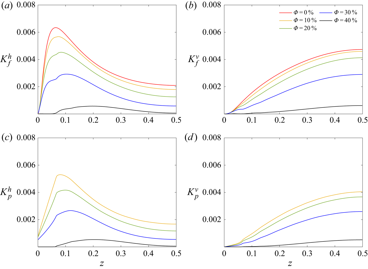
Figure 9. Components of the average kinetic energy per unit mass, derived from the velocity r.m.s., as a function of the vertical direction for the different particle volume fractions indicated. (a) Horizontal and (b) vertical contributions of the fluid, see (3.3a,b); (c) horizontal and, (d) vertical contributions from the particles, defined in (3.4a,b). In all the cases,  $d^*_p=1/15$.
The vertical velocity fluctuations  $K^v_f$ and
  $K^v_p$ are depicted in figures 9(b) and 9(d). These fields reach the maximum value at the centre of the cavity, with very small values close to the walls. Weakening with increasing particle volume fraction is also found for the vertical motions, throughout the cavity. Since the bulk of the cavity is mostly dominated by the ascending and descending thermal plumes that form the upward and downward sections of the large-scale circulation, these results corroborate the notion of a weakened circulation. Combining the different observations drawn from figure 9, it is clear that the overall kinetic energy and the strength of the large-scale circulation decreases everywhere in the cavity with increasing particle volume fraction.
The Reynolds number based on the maximum r.m.s. value of the fluid vertical velocity can act as a measure of the turbulence, induced by the large-scale circulation structures. Figure 10 shows the Reynolds number as a function of the particle volume fraction. The Reynolds number decreases monotonically as the number of particles in the cavity increases. For  $\varPhi \leq 25\,\%$ the decrease is relatively mild, while for larger particle volume fractions the decrease is more pronounced. At
  $\varPhi =40\,\%$, a Reynolds number value of approximately 515 is obtained, almost a third of the single-phase value of 1424. Even though the Reynolds number value at the highest particle volume fraction is significantly decreased, it is not so small as to suggest a complete breakdown of the large-scale circulation. Nonetheless, in line with the Nusselt number reduction and the kinetic energy profiles previously shown, the turbulence induced by the large-scale circulation is rapidly weakened beyond
  $\varPhi =30\,\%$.
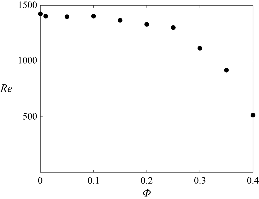
Figure 10. Reynolds number based on the maximum r.m.s. value of the fluid vertical velocity,  $Re=Lw_f^{rms}/\nu$, as a function of the particle volume fraction, for
  $d^*_p=1/15$.
To also analyse the effects of particle rotation, the horizontal (rotation axis in the  $x$–
$x$– $y$ plane) and vertical (rotation axis in the
  $z$-direction) components of the average absolute particle angular velocity
  $|{\omega }_p|$ are shown in figure 11. To conduct the averaging, the vertical direction is split into 30 equal intervals, inside of which the angular velocity of each particle is added and divided by the number of particles inside each specific interval. As with other statistical fields presented in this study, an additional averaging between the symmetric top and bottom locations is performed, resulting in 15 intervals in the vertical direction. A first observation from figure 11 is that the particle rotation decreases with the particle volume fraction. The horizontal component is much larger than its vertical counterpart, and has an important role in the heat transfer process next to the wall: it drags colder fluid closer to the heated wall and hot fluid away from the heated wall (the opposite applies next to the cooled wall). This process contributes to retaining higher heat transfer rates up to
  $\varPhi =30\,\%$ (cf. figure 6a), even though the turbulent activity in the cavity (see the velocity r.m.s. values shown in figure 9) decreases significantly with the particle volume fraction. For the largest particle volume fraction,
  $\varPhi =40\,\%$, where the boundary layers are covered with a tightly packed layer of particles, the rotation next to the walls further diminishes, causing the significant decrease of the Nusselt number reported above, see figure 6(a).

Figure 11. Average particle angular velocity as a function of the vertical direction. (a) Horizontal component and (b) vertical component. In all the cases,  $d^*_p=1/15$.
To provide further evidence on the role of particle rotation in sustaining the heat transfer, three additional simulations were conducted where particles are not allowed to rotate, but just translate. The volume fractions considered for this analysis are  $\varPhi =10\,\%$, 20 % and 30 % and
  $d^*_p=1/15$. First, we compare in figure 12 the Nusselt number for the cases with and without particle rotation. As in § 3.2, the Nusselt number is calculated by averaging the corresponding values at the bottom and top walls. For all three particle volume fractions, the Nusselt number is reduced when particles are not allowed to rotate. This reduction increases with the particle volume fraction, exceeding 30 % reduction at
  $\varPhi =30\,\%$. On the other hand, the temperature fluctuations in the fluid phase, reported in figure 13(a), exhibit the opposite trend, with the maximum values increasing as the particle volume fraction increases. This observation reveals another aspect of particle rotation, the rotation-induced thermal mixing, the absence of which leads to increase temperature inhomogeneities in the cavity, and therefore increased temperature fluctuations. Finally, the horizontal component of the fluid kinetic energy, is shown in figure 13(b). In contrast to the temperature fluctuations, the kinetic energy decreases when rotation is not allowed, revealing the importance of particle rotation for the overall turbulence production inside the cavity, see also Costa et al. (Reference Costa, Picano, Brandt and Breugem2018) and Brandt & Coletti (Reference Brandt and Coletti2022) for the case of pressure-driven channel flows.

Figure 12. Nusselt number of the suspensions for cases with and without particle rotation, as a function of the particle volume fraction, for  $d_p^*=1/15$.

Figure 13. Comparison between simulations where particle rotation is allowed and when it is not allowed. (a) Temperature r.m.s. of the fluid phase and (b) horizontal contribution of the kinetic energy per unit mass of the fluid. In all the cases,  $d_p^*=1/15$.
3.4. TKE budgets
A TKE budget analysis is given here to reveal the role of particles on altering the production and dissipation of TKE. Considering the Navier–Stokes equations with the IBM force ( $\boldsymbol {f}$) employed to impose no slip at the particle surface, the TKE budget can be written for a steady state turbulent flow (
 $d K / dt = 0$) as
 $$\begin{gather} \frac{\partial \mathcal{T}_i}{\partial x_i} = \mathcal{P} - \mathcal{\epsilon} + \mathcal{I}, \end{gather}$$
 $$\begin{gather}\mathcal{P} = \langle [1-{\beta}_f({T}_f-{T}_0)] g u_i \delta_{i3} \rangle, \end{gather}$$
 $$\begin{gather}\mathcal{\epsilon} = \nu \left\langle \frac{\partial u_i }{\partial x_j } \frac{\partial u_i }{\partial x_j} \right\rangle, \end{gather}$$
 $$\begin{gather}\mathcal{I} = \langle u_i f_i \rangle, \end{gather}$$
where  $\mathcal {T}$ is responsible for the spatial redistribution of the kinetic energy,
  $\mathcal {P}$ denotes the production through buoyancy forces,
  $\mathcal {\epsilon }$ refers to the viscous dissipation and finally
  $\mathcal {I}$ is the interphase energy injection via the IBM force (Tanaka & Teramoto Reference Tanaka and Teramoto2015).
Figure 14(a) depicts the profiles of  $\mathcal {P}$,
  $\mathcal {\epsilon }$ and
  $\mathcal {I}$ at different volume fractions, for
  $d^*_p=1/15$. Similarly, the spatial redistribution term in the wall-normal direction is given in figure 14(b). Interestingly, the dissipation is reduced significantly with the volume fraction in the immediate vicinity of the wall, while the production is almost unchanged in that region. In the regions further away from the wall, both production and dissipation are reduced with increasing particle volume fraction. This is consistent with the attenuation in overall TKE, reported in figure 9. It should be noted that the interphase energy injection
  $\mathcal {I}$ is several orders of magnitude smaller than the other terms and its effect can be neglected here. A closer look at figure 14(b) reveals a local minimum in the spatial redistribution term, located just above a particle diameter from the wall, where the particle wall layer ends. This local minimum is emphasised as the particle volume fraction increases, where the particle layering next to the walls is more pronounced. It can be concluded from this analysis that the formation of a particle wall layer close to the wall pulls the generated TKE towards the wall and dissipates it faster through viscous dissipation. This mechanism is in fact more pronounced when the particle volume fraction is higher.

Figure 14. TKE budgets for different particle volume fractions, as a function of the vertical direction. (a) Solid lines, production ( $\mathcal {P}$); dashed lines, dissipation (
 $\epsilon$); dashed-dotted lines, interface injection (
 $\mathcal {I}$). (b) Redistribution term in the wall-normal direction (
 $\partial \mathcal {T}_z/\partial z$). In all the cases,
  $d^*_p=1/15$.
With the availability of the TKE dissipation, the Kolmogorov-based Stokes number  $St_{K}=d_p^2\epsilon ^{1/2}/(18\nu ^{3/2})$ can be calculated. In the range
  $\varPhi <30\,\%$, an approximately constant value of
  $St_{K}=3.9$ is obtained. At higher particle volume fractions it decreases to
  $St_{K}=3.5$ at
  $\varPhi =35\,\%$ and
  $St_{K}=3.0$ at
  $\varPhi =40\,\%$. Even though the Stokes number reduction is not pronounced, it does suggest the increasing impact of the turbulent fluctuations on the particle movement as the particle volume fraction increases.
3.5. Heat transfer budgets
To provide further insight in the heat transfer mechanisms inside the cavity, we present in this section the analysis of the heat transfer budgets. The phase-ensemble procedure adopted in this study allows us to express the different contributions to the total heat flux inside the cavity as a function of the wall-normal direction. Following the derivations in Ardekani et al. (Reference Ardekani, Abouali, Picano and Brandt2018a) and Yousefi et al. (Reference Yousefi, Ardekani, Picano and Brandt2021), one can obtain the following relation:
 \begin{align} q''_{tot}(z) &=
\left(1-\left\langle \varphi\right\rangle_{x,y,t}\right)
\left(\left\langle \frac{{\rm d} T_f}{{\rm d}
z}\right\rangle_{x,y,t} -\sqrt{\mathrm{Ra}\mathrm{Pr}}
\langle w'_f T'_f\rangle_{x,y,t} \right)
\nonumber\\ &\quad +\left\langle
\varphi\right\rangle_{x,y,t}\left(\left\langle \frac{{\rm
d} T_p}{{\rm d} z}\right\rangle_{x,y,t}
-\sqrt{\mathrm{Ra}\mathrm{Pr}} \langle w'_p
T'_p\rangle_{x,y,t} \right),
\end{align}
\begin{align} q''_{tot}(z) &=
\left(1-\left\langle \varphi\right\rangle_{x,y,t}\right)
\left(\left\langle \frac{{\rm d} T_f}{{\rm d}
z}\right\rangle_{x,y,t} -\sqrt{\mathrm{Ra}\mathrm{Pr}}
\langle w'_f T'_f\rangle_{x,y,t} \right)
\nonumber\\ &\quad +\left\langle
\varphi\right\rangle_{x,y,t}\left(\left\langle \frac{{\rm
d} T_p}{{\rm d} z}\right\rangle_{x,y,t}
-\sqrt{\mathrm{Ra}\mathrm{Pr}} \langle w'_p
T'_p\rangle_{x,y,t} \right),
\end{align}
where  $w'=w(t)-\left \langle w\right \rangle$ and
  $T'=T(t)-\left \langle T\right \rangle$ are the fluctuations of the vertical velocity and temperature. The total heat flux can be split into diffusion and convection in each phase
 \begin{equation} \left.\begin{gathered} C_f ={-} \left(1-\left\langle \varphi\right\rangle_{x,y,t}\right)\sqrt{{Ra}\,{Pr}} \left\langle w'_f T'_f\right\rangle_{x,y,t},\quad D_f = \left(1-\left\langle \varphi\right\rangle_{x,y,t}\right) \left\langle \frac{{\rm d} T_f}{{\rm d} z}\right\rangle_{x,y,t}, \\ C_p ={-} \left\langle \varphi\right\rangle_{x,y,t} \sqrt{{Ra}\,{Pr}} \left\langle w'_p T'_p\right\rangle_{x,y,t},\quad D_p = \left\langle \varphi\right\rangle_{x,y,t}\left\langle \frac{{\rm d} T_p}{{\rm d} z}\right\rangle_{x,y,t}, \end{gathered}\right\} \end{equation}
where  $C$ expresses the convection and
  $D$ the diffusion components in the fluid and particles.
The wall-normal distributions of the normalised heat transfer budgets are shown in figure 15 for different particle volume fractions and  $d^*_p=1/15$. As expected, the region close to the wall is mainly dominated by diffusion, while the bulk of the cavity is dominated by turbulent convection. In the fluid phase, the contribution of convection decreases as the particle volume fraction increases, with a dramatic decrease for
  $\varPhi =40\,\%$ in the
  $z<0.1$ region. On the other hand, the relative contribution of fluid diffusion increases, more significantly for
  $\varPhi =40\,\%$, with a pronounced maximum at approximately one particle diameter from the wall. As regards the heat transfer in the particle phase, increasing the particle volume fraction results in an increase of the contributions to the total transport, with the exception of convection at
  $\varPhi =40\,\%$ that decreases in a similar fashion as in the fluid phase. Most notably, the normalised particle diffusion increases significantly next to the walls for
  $\varPhi =40\,\%$, reflecting the dense layering of particles in that location.

Figure 15. Normalised contributions of the heat transfer budgets for different particle volume fractions as a function of the wall-normal direction. (a) Convection by the fluid velocity fluctuations; (b) molecular diffusion in the fluid phase; (c) convection by the particle velocity fluctuations and (d) molecular diffusion in the particle phase. In all the cases,  $d^*_p=1/15$.
Figure 16 presents the aggregated heat transfer budget, in the form of total convection and total diffusion in the two phases; note that the sum of the two is constant across the cavity and equal to the total heat transfer for each case, quantified earlier by the Nusselt number. Interestingly, the significant drop in kinetic energy with increasing particle volume fraction (depicted in figure 9), is not reflected in the convection budgets, which are only slightly affected up to  $\varPhi =30\,\%$. This is mainly attributed to the increasing temperature fluctuations (shown in figure 8) that overcome the decreasing kinetic agitation and retain the intensity of convection heat transfer. Furthermore, the data show that the largest contribution to the heat transfer from turbulent convection in the bulk and, consequently, diffusion in the near-wall region occurs for
  $\varPhi =20\,\%$. A similar behaviour is also observed for
  $\varPhi =10\,\%$ and
  $30\,\%$. Conversely, the
  $\varPhi =40\,\%$ case exhibits a significant decrease of the convection in the bulk (reflected in the significant reduction of the Nusselt number); in this case, the shift between convective and diffusive transport does not occur in the close vicinity of the wall as for the lower values of
  $\varPhi$, but already for
  $z<0.1$, where a plateau is formed. In this region, the total contribution from diffusion is larger for
  $\varPhi =40\,\%$ than for the other cases, except from the region very close to the wall where the lower particle volume fraction cases have significantly larger diffusion. These results quantify the effect of the tightly packed layer of particles next to the walls at
  $\varPhi =40\,\%$, which significantly influences all heat transfer budgets.

Figure 16. Convective and diffusive contributions to the total heat transfer for different particle volume fractions. (a) Convection by both the fluid and particle velocity fluctuations and (b) molecular diffusion in both phases. In all the cases,  $d^*_p=1/15$.
3.6. Two-point correlations
To study the effects of particle volume fraction on the fluid structures inside the cavity, the two-point spatial correlations of the velocity fluctuations along the horizontal directions are presented. These correlations are calculated as
 \begin{equation} \left.\begin{gathered}
R^{x}_{uu}\left(\Delta x,z\right)= \frac{\langle
u'(x,y,z,t)u'(x+\Delta
x,y,z,t)\rangle}{\langle
(u'(x,y,z,t))^2\rangle}, \\
R^{y}_{uu}(\Delta y,z)= \frac{\langle
u'(x,y,z,t)u'(x,y+\Delta
y,z,t)\rangle}{\langle
(u'(x,y,z,t))^2\rangle},
\end{gathered}\right\}
\end{equation}
\begin{equation} \left.\begin{gathered}
R^{x}_{uu}\left(\Delta x,z\right)= \frac{\langle
u'(x,y,z,t)u'(x+\Delta
x,y,z,t)\rangle}{\langle
(u'(x,y,z,t))^2\rangle}, \\
R^{y}_{uu}(\Delta y,z)= \frac{\langle
u'(x,y,z,t)u'(x,y+\Delta
y,z,t)\rangle}{\langle
(u'(x,y,z,t))^2\rangle},
\end{gathered}\right\}
\end{equation}
and likewise for  $R^{x}_{vv}(\Delta x,z)$,
  $R^{y}_{vv}(\Delta y,z)$,
  $R^{x}_{ww}(\Delta x,z)$ and
  $R^{y}_{ww}(\Delta y,z)$. Taking into account that the horizontal
  $x$ and
  $y$ directions are homogeneous, some correlations are statistically equivalent, more specifically
  $(R^{x}_{uu},R^{y}_{vv})$,
  $(R^{x}_{vv},R^{y}_{uu})$ and
  $(R^{x}_{ww},R^{y}_{ww})$ are equivalent in pairs. Since the near-wall region is dominated by the horizontal sweeping flow of the large-scale circulation, the correlation groups
  $(R^{x}_{uu},R^{y}_{vv})$ and
  $(R^{x}_{vv},R^{y}_{uu})$ provide information about the shape and degree of coherence of these horizontal flow structures. Conversely,
  $(R^{x}_{ww},R^{y}_{ww})$ provides similar information for the vertical flow structures in the bulk of the cavity, which is dominated by the ascending and descending plumes that fuel the large-scale circulation.
Figure 17 shows these three groups of two-point correlation functions for  $\varPhi =0\,\%$, 35 % and 40 %, with
  $d^*_p=1/15$. The other cases are omitted because they are qualitatively similar to cases
  $\varPhi =0\,\%$ and 35 %. As expected, the correlation
  $(R^{x}_{ww}+R^{y}_{ww})/2$ (first row in the figure) becomes larger in the bulk of the cavity, while
  $(R^{x}_{uu}+R^{y}_{vv})/2$ and
  $(R^{x}_{vv}+R^{y}_{uu})/2$ (second and third rows) are larger closer to the walls. Focusing on the differences between
  $\varPhi =0\,\%$ and 35 % (first and second columns), it is clear that the degree of correlation increases with increasing particle volume fraction and therefore the flow structures become coherent over larger distances. This observation indicates a change in the shape of the fast-moving periphery of the large-scale circulation, which becomes thicker with increasing particle volume fraction. It is also evident that the most correlated regions move further away from the wall, something that is more clearly depicted when comparing the
  $(R^{x}_{uu}+R^{y}_{vv})/2$ values in figures 17(d) and 17(e). This is related to the increase of the local particle volume fraction close to the walls which increasingly limits the access of the large-scale circulation to this region. For the largest volume fraction examined,
  $\varPhi =40\,\%$, a significant difference is immediately visible: up to a height of approximately one particle diameter the correlation lengths of all two-point correlation functions are minimal. The packed layer of particles in this region breaks up any correlations in the fluid and moves the flow structures outside this particle layer.

Figure 17. Contour plots of the two-point velocity correlations. Panels show (a–c)  $(R^{x}_{ww}+R^{y}_{ww})/2$; (d–f)
  $(R^{x}_{uu}+R^{y}_{vv})/2$; and (g–i)
  $(R^{x}_{vv}+R^{y}_{uu})/2$. For (a,d,g)
  $\varPhi =0\,\%$; (b,e,h)
  $\varPhi =35\,\%$; and (c, f,i)
  $\varPhi =40\,\%$. In all the cases,
  $d^*_p=1/15$. Since the
  $x$- and
  $y$-directions are homogeneous and the two-point correlations are statistically equivalent in pairs, the results shown here are also valid if
  $\Delta x$ is replaced with
  $\Delta y$ in the
  $x$-axis of the figure.
3.7. Effects of particle size
Following the parametric study of the particle volume fraction presented in the previous sections, this section focuses on the effects of the particle size. Three dimensionless particle diameters are used,  $d^*_p=1/20$, 1/15 and 1/10, for a particle volume fraction of 35 %. These values correspond to a free-fall-based Stokes number of
  $St_f=0.5$, 0.9 and 2.1, and a Kolmogorov-based Stokes number of
  $St_K=1.1$, 3.5 and 8.1 respectively. The values of both definitions of the Stokes number suggest an increasing influence of the particle inertia relative to the large- and small-scale flow features as the particle size increases.
First, the Nusselt number and thermal boundary layer thickness are shown in figure 18 as a function of the dimensionless particle diameter. As the size of the particle decreases, the Nusselt number decreases significantly and, correspondingly, the thermal boundary layer thickness increases. This weakening of the heat transfer inside the cavity is as dramatic as the Nusselt decrease observed in § 3.2 for  $\varPhi =40\,\%$ and
  $d^*_p=1/15$. The main difference observed here is the fact that the r.m.s.-based definition of the thermal boundary layer thickness follows the gradient-based definition very closely, in contrast to the findings in § 3.2 where the two definitions deviate.

Figure 18. (a) Nusselt number and (b) thermal boundary layer thickness as a function of the dimensionless particle diameter, for  $\varPhi =35\,\%$. The boundary layer thickness based on the gradient is defined in (3.1) and the r.m.s.-based definition given in (3.2). Both quantities are calculated by averaging the relevant quantities at the bottom and top walls.
To provide more insight into this pronounced drop in heat transfer, figure 19 visualises the first particle layer next to the bottom wall. As the particles decrease in size they cluster in the near-wall region, forming a tightly packed layer for  $d^*_p=1/20$. In addition, the particle temperature increases, suggesting that the particles remain in the near-wall region for an extended time period. The particle distribution inside the cavity is presented in figure 20, in the form of averaged local particle volume fraction as a function of the vertical direction
  $z$. All three cases share similar characteristics, with a maximum close to the wall and approximately uniform distribution in the bulk of the cavity. As the particle size decreases, the maximum value becomes larger and moves closer to the wall. The maximum values for all the cases occur just above half a particle diameter from the walls. Again, the results for the case with the smallest particles are very similar to what is observed in figure 7 for
  $\varPhi =40\,\%$ and
  $d^*_p=1/15$. In both these cases, the local particle volume fraction exceeds the value 80 % close to the wall. The increased layering next to the walls for smaller particles was also observed in turbulent channel flows (Costa et al. Reference Costa, Picano, Brandt and Breugem2018), albeit not as distinctly as the present study. This finding points to the fact that the strong wall–particle lubrication interaction is more effective with smaller particles, inducing the formation of denser layers next to the walls, influencing the boundary layer region more intensely.
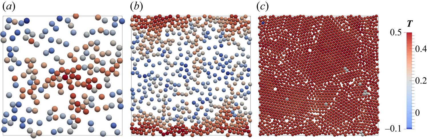
Figure 19. Snapshots of the first particle layer next to the bottom wall ( $x$–
$x$– $y$ plane). The particles are coloured based on their temperature; (a)
  $d^*_p=1/10$, (b)
  $d^*_p=1/15$ and (c)
  $d^*_p=1/20$. In all the cases,
  $\varPhi =35\,\%$.

Figure 20. Average local particle volume fraction as a function of the vertical direction for different values of the dimensionless particle diameter. In all the cases,  $\varPhi =35\,\%$.
Further analysing the effects of particles with different sizes, figure 21 shows the average kinetic energy per unit mass, as a function of the vertical direction. The most interesting observation is the diminished horizontal contribution to the kinetic energy of both the fluid and particles (figure 21a,c) in the region  $z<0.05$, for the case with the smallest particles. This region corresponds to the dense particle layer forming next to the wall, hindering both the fluid and particle movement. Combining this with the decreased vertical contributions (figure 21b,d) in the cavity core, indicates the weakening of the large-scale circulation structure, much similar to the highest particle volume fraction results presented in § 3.3.3.

Figure 21. Components of the average kinetic energy per unit mass, derived from the velocity r.m.s., as a function of the vertical direction for the different dimensionless particle diameters indicated. (a) Horizontal and (b) vertical contributions of the fluid, see (3.3a,b); (c) horizontal and (d) vertical contributions from the particles, defined in (3.4a,b).
Focusing further on the heat transfer inside the cavity, figure 22 presents the convective and diffusive contributions to the total heat transfer. As the particle size decreases, both the convective contributions (dominating the bulk of the cavity) and the diffusive contributions (dominating the near-wall region) decrease. Similar to the Nusselt number variation, the case with the smallest particles exhibits the most pronounced reduction. The convective contributions are diminished in the particle packed region  $z<0.05$, while the diffusive contributions are approximately uniform in this region. The similarities to figure 16 for the largest particle volume fraction and
  $d^*_p=1/15$ are once again distinct, indicating the dominance of diffusive heat transfer throughout the tightly packed particle layer.

Figure 22. Convective and diffusive contributions to the total heat transfer for different dimensionless particle diameters. (a) Convection by both the fluid and particle velocity fluctuations and (b) molecular diffusion in both phases.
4. Conclusions
We present and discuss direct numerical simulations of Rayleigh–Bénard convection in non-colloidal suspensions, with a special focus on the heat transfer modulation with increasing particle volume fraction and particle size. The suspended particles are neutrally buoyant, with all thermophysical properties matching the properties of the fluid. We employed direct-forcing IBM to fully resolve the fluid–solid interactions coupled with a VoF approach to solve the temperature equation in the two phases and to characterise the flow statistics.
At the macroscopic level, the Nusselt number is shown to weakly increase up to  $\varPhi =25\,\%$ and then significantly drop beyond that point. The positive effect of the particles on the Nusselt number for
  $\varPhi \leq 25\,\%$ originates from increased thermal agitation that overcomes the decreased flow kinetic energy in the cavity. For higher volume fractions, both the instantaneous snapshots of the flow and the statistical analysis revealed an increased layering of particles next to the walls, reaching local volume fractions over 80 %, indicating an almost fully packed layer. As a consequence, the ejection of thermal plumes from the boundary layers and the heat transfer inside the cavity are considerably weakened. Significant differences between the case with
  $\varPhi =40\,\%$ and the rest of the cases are observed throughout the statistical quantities presented, including the TKE and heat transfer budgets, and the two-point correlation functions. The role of particle rotation on the heat transfer modulation is further investigated with additional simulations, considering particles without the ability to rotate. In this setting, the thermal agitation increases while the kinetic energy in the cavity decreases when comparing with the cases where rotation is allowed. The overall effect on the heat transfer is weakening, with the Nusselt number decreasing significantly from
  $\varPhi >30\,\%$. This observation highlights the role of rotation in counteracting the decrease of the heat transfer as the number of particles in the flow increases.
Studying the effects of the particle size reveals a strong heat transfer reduction with smaller particles. This reduction can be attributed to the increased layering next to the walls, which suggests that the strong wall–particle lubrication interaction is more effective for smaller particles. In general, decreasing the particle size affects the heat transfer and the other statistical quantities in a similar fashion as the increase in particle volume fraction. The influence of the particle size on the critical volume fraction (the volume fraction above which heat transfer reduces) should be the topic of a future study. Guided by the observation that the heat transfer reduction is associated with nearly fully packed wall layers, new simulations can be designed to quantify the functional dependence of the critical volume fraction on the particle size.
Our study quantifies the effects of non-colloidal particle suspensions in turbulent Rayleigh–Bénard convection. An exciting prospect for the continuation of this research will be to perform experiments to verify the inhomogeneity in the variation of Nusselt number, temperature and particle concentration distributions especially for the higher particle volume fractions studied here. Other interesting future extensions of this work would be to extend the parameter space to higher Rayleigh numbers, where turbulence is stronger, and change key characteristics of the particles, such as shape and thermophysical properties.
Funding
The research was financially supported by the Swedish Research Council, via the multidisciplinary research environment INTERFACE (VR 2016-06119 ‘Hybrid multiscale modelling of transport phenomena for energy efficient processes’). The computation resources were provided by SNIC (Swedish National Infrastructure for Computing) and by the National Infrastructure for High Performance Computing and Data Storage in Norway (project no. NN9561K). P.M. has been supported in part by the National Science Foundation Award No. 1854376 and in part by the Army Research Office Award No. W911NF-18-1-0356.
Declaration of interests
The authors report no conflict of interest.