1 Introduction
The exchange of heat and salt across the turbulent boundary layer at the ice–ocean interface governs the rate at which sea ice and ice shelves melt or grow in response to changes in ocean properties. Estimates of the heat exchange at such interfaces vary substantially across observational and modelling studies. In order to predict the evolution of sea ice and ice shelves more accurately, better constraints on their heat exchange with the underlying ocean are needed.
Antarctica is surrounded by ice shelves, thick floating sheets of ice that extend from the grounding line onto the ocean surface. They play a critical role in the mass balance and dynamics of Antarctica’s terrestrial ice by serving as a buttress at the coastline and limiting the rate of ice flow into the ocean (Hooke Reference Hooke2005). Antarctic ice shelves are also important to the formation of Antarctic Bottom Water, a mass of dense water that fills approximately one half of the deep ocean (Broecker et al. Reference Broecker, Peacock, Walker, Weiss, Fahrbach, Schröder, Mikolajewicz, Heinze, Key and Peng1998) and that plays an important role in the carbon cycle (Marinov et al. Reference Marinov, Gnanadesikan, Sarmiento, Toggweiler, Follows and Mignone2008).
Recent studies show that warm and salty Circumpolar Deep Water around Antarctica is shoaling onto the continental shelf and intruding into the ocean cavities under ice shelves, causing increased melting of their basal surfaces (Jacobs et al. Reference Jacobs, Jenkins, Giulivi and Dutrieux2011; Pritchard et al. Reference Pritchard, Ligtenberg, Fricker, Vaughan, Van den Broeke and Padman2012; Schmidtko et al. Reference Schmidtko, Heywood, Thompson and Aoki2014). This process is depicted in figure 1. Increased basal melting can trigger the disintegration of ice shelves (Feldmann & Levermann Reference Feldmann and Levermann2015) and hence accelerate Antarctic ice loss, which would contribute significantly to global sea level rise. The rough topography of the ocean floor under ice shelves may play a role in guiding the warm shoaling water inside the cavity (Brisbourne et al. Reference Brisbourne, Smith, King, Nicholls, Holland and Makinson2014). Basal melting results in a buoyant plume of meltwater that flows along the shelf base, generating turbulence, which in turn affects both the transfer of heat to the shelf and the entrainment of heat from the relatively warm far field into the relatively cold boundary layer (Little, Gnanadesikan & Hallberg Reference Little, Gnanadesikan and Hallberg2008).

Figure 1. Warm Circumpolar Deep Water (CDW) rising into the ocean cavity under an Antarctic ice shelf.
Previous studies of ice shelf–ocean interaction have been conducted mainly through numerical models. The heat transfer from the ocean mixed layer to the ice shelf base in these models is parameterized in terms of the temperature difference across, and the thermal exchange velocity
 ${\it\gamma}_{T}$
through, the boundary layer.
${\it\gamma}_{T}$
through, the boundary layer.
 ${\it\gamma}_{T}$
is defined as the ratio of the thermal diffusivity to the thickness of the boundary layer. In the earlier works of Hellmer & Olbers (Reference Hellmer and Olbers1989) and Scheduikat & Olbers (Reference Scheduikat and Olbers1990),
${\it\gamma}_{T}$
is defined as the ratio of the thermal diffusivity to the thickness of the boundary layer. In the earlier works of Hellmer & Olbers (Reference Hellmer and Olbers1989) and Scheduikat & Olbers (Reference Scheduikat and Olbers1990),
 ${\it\gamma}_{T}$
was taken to be a constant. Jenkins (Reference Jenkins1991) followed the theory of Kader & Yaglom (Reference Kader and Yaglom1972), assuming that the ice–water interface is hydraulically smooth, and expressed
${\it\gamma}_{T}$
was taken to be a constant. Jenkins (Reference Jenkins1991) followed the theory of Kader & Yaglom (Reference Kader and Yaglom1972), assuming that the ice–water interface is hydraulically smooth, and expressed
 ${\it\gamma}_{T}$
in terms of the friction velocity of the turbulent boundary layer. This formulation was used in the studies by Holland & Feltham (Reference Holland and Feltham2006) and Jenkins, Nicholls & Corr (Reference Jenkins, Nicholls and Corr2010b
). McPhee, Maykut & Morison (Reference McPhee, Maykut and Morison1987) developed a parameterization for
${\it\gamma}_{T}$
in terms of the friction velocity of the turbulent boundary layer. This formulation was used in the studies by Holland & Feltham (Reference Holland and Feltham2006) and Jenkins, Nicholls & Corr (Reference Jenkins, Nicholls and Corr2010b
). McPhee, Maykut & Morison (Reference McPhee, Maykut and Morison1987) developed a parameterization for
 ${\it\gamma}_{T}$
by using the formulation of Yaglom & Kader (Reference Yaglom and Kader1974) for the transfer of heat in a turbulent boundary layer near a rough wall and by additionally considering the effect of buoyancy and rotation on heat transfer. Holland & Jenkins (Reference Holland and Jenkins1999), Mueller et al. (Reference Mueller, Padman, Dinniman, Erofeeva, Fricker and King2012) and Dansereau, Heimbach & Losch (Reference Dansereau, Heimbach and Losch2014) adopted this parameterization in their studies. The formation of channels in the ice shelf base as a result of plumes flowing on the underside of the shelf has also been investigated numerically (Dallaston, Hewitt & Wells Reference Dallaston, Hewitt and Wells2015).
${\it\gamma}_{T}$
by using the formulation of Yaglom & Kader (Reference Yaglom and Kader1974) for the transfer of heat in a turbulent boundary layer near a rough wall and by additionally considering the effect of buoyancy and rotation on heat transfer. Holland & Jenkins (Reference Holland and Jenkins1999), Mueller et al. (Reference Mueller, Padman, Dinniman, Erofeeva, Fricker and King2012) and Dansereau, Heimbach & Losch (Reference Dansereau, Heimbach and Losch2014) adopted this parameterization in their studies. The formation of channels in the ice shelf base as a result of plumes flowing on the underside of the shelf has also been investigated numerically (Dallaston, Hewitt & Wells Reference Dallaston, Hewitt and Wells2015).
There are numerous laboratory experiments on heat transfer at a phase change boundary between a solid and a liquid that are relevant to our study. Townsend (Reference Townsend1964) investigated the evolution of the layer of free convection over an ice surface into a stable liquid layer above. The instability of an ice surface, and subsequent formation of a wavy interface, in the presence of a turbulent flow was explored by Gilpin, Hirata & Cheng (Reference Gilpin, Hirata and Cheng1980). Significant work has been performed on the study of the formation of a mushy layer and on compositional and thermal convection in the liquid during the solidification of a binary solution to explain brine rejection as sea ice forms (Huppert & Worster Reference Huppert and Worster1985; Wettlaufer, Worster & Huppert Reference Wettlaufer, Worster and Huppert1997). The effect of an external shear flow on a mushy layer has also been investigated (Neufeld & Wettlaufer Reference Neufeld and Wettlaufer2008). In the latter study, a laminar shear flow was applied to an
 $\text{NH}_{4}\text{Cl}$
mushy layer from above and the primary focus was the stability of the mushy layer in response to the shear flow. Kerr & McConnochie (Reference Kerr and McConnochie2015) developed a theoretical model for the dissolution of a vertical solid surface and tested their model with experimental measurements. These laboratory studies provide an explanation of the physical processes at an ice–water interface and are useful guides for investigating the effect of turbulent warm water at an ice–ocean interface. Also related to ice shelf–ocean interaction is the set of experiments by Stern et al. (Reference Stern, Holland, Holland, Jenkins and Sommeria2014) on the effect of geometry on circulation inside the ice shelf cavity and at the ice shelf front. None of these studies, however, consider the effect of shear-driven turbulence on what is essentially a horizontal ice shelf–ocean interface.
$\text{NH}_{4}\text{Cl}$
mushy layer from above and the primary focus was the stability of the mushy layer in response to the shear flow. Kerr & McConnochie (Reference Kerr and McConnochie2015) developed a theoretical model for the dissolution of a vertical solid surface and tested their model with experimental measurements. These laboratory studies provide an explanation of the physical processes at an ice–water interface and are useful guides for investigating the effect of turbulent warm water at an ice–ocean interface. Also related to ice shelf–ocean interaction is the set of experiments by Stern et al. (Reference Stern, Holland, Holland, Jenkins and Sommeria2014) on the effect of geometry on circulation inside the ice shelf cavity and at the ice shelf front. None of these studies, however, consider the effect of shear-driven turbulence on what is essentially a horizontal ice shelf–ocean interface.
In this paper, we describe an experimental study on the response of an ice–water interface to forced convection in the form of turbulent mixing in pure water over ice. The experiments are conducted in a cylindrical tank with a layer of ice growing on a basal cooling plate at the bottom, representing the base of an ice shelf. The overlying water layer is covered at the top by a lid with a rough underside. This rough surface drives the motion in the water column and creates a well-mixed turbulent liquid layer when the lid is rotated. Turbulent mixing causes warm water to be transported from the far field to the ice–water interface. Our laboratory set-up is an idealized, inverted model of the ocean cavity under Antarctic ice shelves in which the circulation of relatively warm water is reaching the basal surface of these ice shelves, causing accelerated basal melting. The set-up is inverted because the boundary layer at the ice–water interface in the experiments is denser than the far field, whereas in the ocean, the boundary layer is relatively buoyant. There is no natural convection in our experiments and hence the boundary layer is stable in the absence of turbulent mixing.
An important difference between the laboratory set-up and the oceanographic case is the absence of salt in the experiments. The ice–ocean interface is at a temperature intermediate between the salinity-dependent freezing point of the ocean and the melting point of ice in fresh water (0 °C). The rate of phase change at the ice–ocean interface is governed by both the conservation of heat and the conservation of salt at the interface. When there is a large heat flux through the boundary layer to the ice–ocean interface, melting occurs. When the liquid far-field temperature is below the melting point of ice at the interface and the interface salinity is non-zero, conservation of salt at the interface causes ice to dissolve (Wells & Worster Reference Wells and Worster2011; Kerr & McConnochie Reference Kerr and McConnochie2015). In this experimental study, we ignore the effect of salinity on the interface temperature, and we focus uniquely on the phase change due to heat transfer, melting.
We formulate a theoretical model for the evolution of the ice thickness in our experiments and compare our measurements with the prediction from our theoretical model in order to develop a parameterization for the turbulent heat transfer at the ice–water interface. The apparatus and procedure are described in § 2. In § 3, the governing equations in our theoretical model are outlined. The results from the set of experiments are shown in § 4 and are compared to the theoretical model in § 5. In § 6, we discuss the geophysical application of our results. Finally, we summarize our study in § 7.
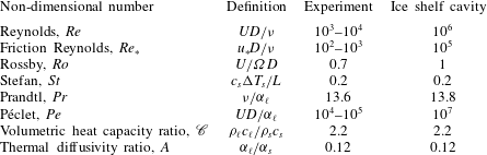
The dimensionless control parameters that are relevant to the study are the Reynolds number, friction Reynolds number, Rossby number and Stefan number. The definition of these parameters and their estimated values in our experiments and in an ice shelf cavity are listed in table 1. In the definitions, the subscript
 $s$
refers to the solid (ice) and the subscript
$s$
refers to the solid (ice) and the subscript
 $\ell$
refers to the liquid (water).
$\ell$
refers to the liquid (water).
 $D$
denotes the depth of the liquid layer;
$D$
denotes the depth of the liquid layer;
 $U$
, the characteristic velocity scale;
$U$
, the characteristic velocity scale;
 $u_{\ast }$
, the friction velocity;
$u_{\ast }$
, the friction velocity;
 ${\it\nu}$
, the kinematic viscosity;
${\it\nu}$
, the kinematic viscosity;
 ${\it\Omega}$
, the angular frequency of rotation;
${\it\Omega}$
, the angular frequency of rotation;
 ${\it\rho}$
, the density;
${\it\rho}$
, the density;
 $c$
, the specific heat capacity;
$c$
, the specific heat capacity;
 ${\rm\Delta}T$
, the temperature difference;
${\rm\Delta}T$
, the temperature difference;
 $L$
, the specific latent heat; and
$L$
, the specific latent heat; and
 ${\it\alpha}$
, the thermal diffusivity.
${\it\alpha}$
, the thermal diffusivity.

Figure 2. Schematic diagram of the apparatus.
Table 1. Dimensionless control parameters in the experiment and in an ice shelf cavity.

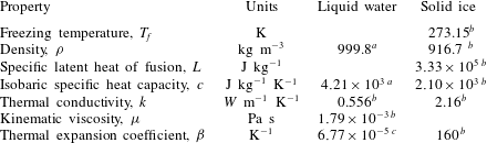
Table 2. Physical properties of liquid water and ice at standard atmospheric pressure.
 ${\it\rho}$
,
${\it\rho}$
,
 $L$
,
$L$
,
 $c$
,
$c$
,
 $k$
,
$k$
,
 ${\it\mu}$
and
${\it\mu}$
and
 ${\it\beta}$
at 273.15 K.
${\it\beta}$
at 273.15 K.
 ${\it\beta}$
for liquid water is linear and
${\it\beta}$
for liquid water is linear and
 ${\it\beta}$
for solid ice is volumetric.
${\it\beta}$
for solid ice is volumetric.
 $^{a}$
From Wagner & Pruß (Reference Wagner and Pruss2002),
$^{a}$
From Wagner & Pruß (Reference Wagner and Pruss2002),
 $^{b}$
from Haynes (Reference Haynes2015) and
$^{b}$
from Haynes (Reference Haynes2015) and
 $^{c}$
from IOC, SCOR & IAPSO (2010).
$^{c}$
from IOC, SCOR & IAPSO (2010).

2 Experimental method
The experimental apparatus is shown in figure 2. It consists of a cylindrical tank of radius 17.5 cm with 1.5 cm thick Perspex walls and a 5 cm thick aluminium basal cooling plate. The tank is filled with pure water to a height of 10 cm, and ice is grown by circulating cold nitrogen gas inside the basal cooling plate. The physical properties of liquid water and ice are listed in table 2. The interior of the plate consists of two sets of parallel spiral grooves, one set having an inlet at the centre and an outlet near the rim and the other set having an inlet near the rim and an outlet at the centre. This arrangement helps achieve a uniform heat flux through the plate and hence uniform ice growth on its surface. The nitrogen flow rate is held constant at
 $0.14~\text{m}^{3}~\text{min}^{-1}$
within and across experiments. A Perspex cover lid is positioned at the upper surface of the water layer, connected to a gear motor by means of a vertical metal rod. A plastic grid is attached to the underside of the cover lid, creating a rough surface for generating the turbulent shear flow. The grid consists of a lattice of squares, each square having sides of length 1.4 cm and projecting downward beneath the lid a distance of 0.9 cm. The rotation of the cover lid and plastic grid is controlled by the gear motor.
$0.14~\text{m}^{3}~\text{min}^{-1}$
within and across experiments. A Perspex cover lid is positioned at the upper surface of the water layer, connected to a gear motor by means of a vertical metal rod. A plastic grid is attached to the underside of the cover lid, creating a rough surface for generating the turbulent shear flow. The grid consists of a lattice of squares, each square having sides of length 1.4 cm and projecting downward beneath the lid a distance of 0.9 cm. The rotation of the cover lid and plastic grid is controlled by the gear motor.
To start each experiment, the water layer, initially at rest and at room temperature, is suddenly cooled from below by turning on the flow of nitrogen into the basal cooling plate. It typically takes approximately 30 min for ice to begin to nucleate on the basal plate. The ice is allowed to grow for another 30 min, reaching a nearly uniform thickness of 8–12 mm, depending on the initial temperature of the water. The motor is then turned on, rotating the lid and grid at a constant angular velocity, typically for approximately one hour. We experimented with lid angular velocities between 0.27 and
 $1.43~\text{rad}\,\text{s}^{-1}$
, fast enough to generate a turbulent shear flow that extends to within approximately 1.5 cm of the bottom surface of the tank in each case.
$1.43~\text{rad}\,\text{s}^{-1}$
, fast enough to generate a turbulent shear flow that extends to within approximately 1.5 cm of the bottom surface of the tank in each case.

Figure 3. Arrangement of thermistors.
Pictures of the ice are taken from the side of the tank at 1 min intervals with a Nikon D800 camera. The ice thickness is subsequently measured from these pictures using GraphClick, a digitizer software. Seven thermistors are placed on a 5.25 cm long vertical strip starting from the bottom of the tank to measure temperature at the locations shown in figure 3. The strip is placed along the wall of the tank and the thermistors protrude 1 cm into the tank. The thermistors are connected to a data logger. We focus on the ice thickness at a radial distance
 $R=13$
cm from the tank centre, that is, 4.5 cm from the outer wall. This location is a compromise between its proximity to the thermistor chain and its separation from the immediate effects of the outer wall.
$R=13$
cm from the tank centre, that is, 4.5 cm from the outer wall. This location is a compromise between its proximity to the thermistor chain and its separation from the immediate effects of the outer wall.
Both the friction velocity and fluid velocity of the turbulent shear flow are measured over the entire range of lid angular velocities. The average shear stress, and hence friction velocity, is obtained by measuring the torque on the lid with a torque meter. The fluid velocity is obtained from planar particle image velocimetry (PIV) measurements. The water is seeded with nearly spherical glass beads of specific gravity 1.1 and average diameter
 $10~{\rm\mu}\text{m}$
and illuminated with a pulsed Nd:YAG laser sheet. A vertical light sheet is set up along a chord at
$10~{\rm\mu}\text{m}$
and illuminated with a pulsed Nd:YAG laser sheet. A vertical light sheet is set up along a chord at
 $r=R$
to measure the vertical profile of the azimuthal component of the velocity. To measure the radial component of the velocity, a horizontal light sheet is set up to illuminate a sector of the tank’s circular cross-sectional area at different heights above the bottom plate. A high-speed CMOS camera synchronized with the pulsed laser taking double exposure images at a resolution of
$r=R$
to measure the vertical profile of the azimuthal component of the velocity. To measure the radial component of the velocity, a horizontal light sheet is set up to illuminate a sector of the tank’s circular cross-sectional area at different heights above the bottom plate. A high-speed CMOS camera synchronized with the pulsed laser taking double exposure images at a resolution of
 $2048\times 2048$
pixels is oriented vertically above the tank and horizontally to the side of the tank, for imaging the radial flow and azimuthal flow, respectively. The open source software PIVlab (Thielicke & Stamhuis Reference Thielicke and Stamhuis2014) is used to calculate PIV velocities from the exposures. For the determinations of the azimuthal velocity profiles, only a vertical strip at the centre of the images taken from the side, in which the particles move in the plane of the light sheet, is used in the analysis.
$2048\times 2048$
pixels is oriented vertically above the tank and horizontally to the side of the tank, for imaging the radial flow and azimuthal flow, respectively. The open source software PIVlab (Thielicke & Stamhuis Reference Thielicke and Stamhuis2014) is used to calculate PIV velocities from the exposures. For the determinations of the azimuthal velocity profiles, only a vertical strip at the centre of the images taken from the side, in which the particles move in the plane of the light sheet, is used in the analysis.
3 Ice energy balance
The energy (enthalpy) balance in a control volume enclosing the ice with thickness
 $h$
at a time
$h$
at a time
 $t$
shown in figure 4 yields the following relationship:
$t$
shown in figure 4 yields the following relationship:
 $$\begin{eqnarray}\displaystyle \frac{\text{d}E}{\text{d}t}=Q_{p}+Q_{\ell }, & & \displaystyle\end{eqnarray}$$
where
 $E$
is the energy (enthalpy) content of the ice, the subscript
$E$
is the energy (enthalpy) content of the ice, the subscript
 $p$
refers to the plate and
$p$
refers to the plate and
 $Q$
is the heat entering the control volume from the region denoted by its subscript. Considering a one-dimensional energy balance,
$Q$
is the heat entering the control volume from the region denoted by its subscript. Considering a one-dimensional energy balance,
 $E$
and
$E$
and
 $Q_{p}$
can be expressed as
$Q_{p}$
can be expressed as
 $$\begin{eqnarray}\displaystyle E={\it\rho}_{s}c_{s}\int _{0}^{h}\overline{T_{s}}\,\text{d}z-{\it\rho}_{s}Lh & & \displaystyle\end{eqnarray}$$
and
 $$\begin{eqnarray}\displaystyle Q_{p}=-\frac{k_{s}{\rm\Delta}T_{s}}{h}. & & \displaystyle\end{eqnarray}$$
In (3.2) and (3.3),
 $k$
is thermal conductivity and
$k$
is thermal conductivity and
 $T$
is temperature.
$T$
is temperature.
 ${\rm\Delta}T_{s}=T_{f}-T_{p}$
, where
${\rm\Delta}T_{s}=T_{f}-T_{p}$
, where
 $T_{f}$
is the freezing temperature of water (also the temperature of the ice–water interface).
$T_{f}$
is the freezing temperature of water (also the temperature of the ice–water interface).
 $\overline{T_{s}}$
is the average temperature of the ice. Assuming that the temperature varies linearly in the vertical direction through the ice,
$\overline{T_{s}}$
is the average temperature of the ice. Assuming that the temperature varies linearly in the vertical direction through the ice,
 $\overline{T_{s}}=(T_{f}+T_{p})/2$
. Numerical values of the physical properties of water and ice are given in table 2. The first term on the right-hand side in (3.2) can be rewritten as
$\overline{T_{s}}=(T_{f}+T_{p})/2$
. Numerical values of the physical properties of water and ice are given in table 2. The first term on the right-hand side in (3.2) can be rewritten as
 $$\begin{eqnarray}\displaystyle {\it\rho}_{s}c_{s}\int _{0}^{h}\overline{T_{s}}\,\text{d}z={\it\rho}_{s}c_{s}h\left(\frac{{\rm\Delta}T_{s}}{2}+T_{p}\right). & & \displaystyle\end{eqnarray}$$

Figure 4. Control volume around ice.
3.1 No turbulent mixing
When the ice is growing in quiescent water, heat is transferred by conduction. We ignore free convection in the liquid. In this case
 $Q_{\ell }$
is the sum of the conductive heat transfer through and the rate of change of enthalpy of the liquid, so that
$Q_{\ell }$
is the sum of the conductive heat transfer through and the rate of change of enthalpy of the liquid, so that
 $$\begin{eqnarray}\displaystyle Q_{\ell }=\frac{k_{\ell }{\rm\Delta}T_{\ell }}{{\it\delta}}+{\it\rho}_{s}c_{s}T_{f}\frac{\text{d}h}{\text{d}t}, & & \displaystyle\end{eqnarray}$$
where the subscript
 $\ell$
refers to the liquid properties,
$\ell$
refers to the liquid properties,
 ${\it\delta}$
is the thickness of the thermal boundary layer above the ice and
${\it\delta}$
is the thickness of the thermal boundary layer above the ice and
 ${\rm\Delta}T_{\ell }=T_{\infty }-T_{f}$
,
${\rm\Delta}T_{\ell }=T_{\infty }-T_{f}$
,
 $T_{\infty }$
being the temperature of the liquid far field. Introducing
$T_{\infty }$
being the temperature of the liquid far field. Introducing
 $$\begin{eqnarray}\displaystyle {\it\delta}=\frac{{\it\alpha}_{\ell }}{\text{d}h/\text{d}t} & & \displaystyle\end{eqnarray}$$
from the heat balance in a control volume in the liquid region above the ice–water interface, with
 ${\it\alpha}_{\ell }$
given by
${\it\alpha}_{\ell }$
given by
 $$\begin{eqnarray}\displaystyle {\it\alpha}_{\ell }=\frac{k_{\ell }}{{\it\rho}_{\ell }c_{\ell }}, & & \displaystyle\end{eqnarray}$$
the conductive term in (3.5) can be rewritten as
 $$\begin{eqnarray}\displaystyle \frac{k_{\ell }{\rm\Delta}T_{\ell }}{{\it\delta}}={\it\rho}_{\ell }c_{\ell }{\rm\Delta}T_{\ell }\frac{\text{d}h}{\text{d}t}. & & \displaystyle\end{eqnarray}$$
Substitution of (3.2)–(3.5), and (3.8) into (3.1) gives, for the heat balance in the control volume,
 $$\begin{eqnarray}\displaystyle \left({\it\rho}_{s}L+\frac{{\it\rho}_{s}c_{s}{\rm\Delta}T_{s}}{2}+{\it\rho}_{\ell }c_{\ell }{\rm\Delta}T_{\ell }\right)\frac{\text{d}h}{\text{d}t}=\frac{k_{s}{\rm\Delta}T_{s}}{h}+\frac{{\it\rho}_{s}c_{s}h}{2}\frac{\text{d}}{\text{d}t}({\rm\Delta}T_{s}), & & \displaystyle\end{eqnarray}$$
which can be approximated, based on the largest terms, as
 $$\begin{eqnarray}\displaystyle ({\it\rho}_{s}L+{\it\rho}_{\ell }c_{\ell }{\rm\Delta}T_{\ell })\frac{\text{d}h}{\text{d}t}\simeq \frac{k_{s}{\rm\Delta}T_{s}}{h}. & & \displaystyle\end{eqnarray}$$
This equation is non-dimensionalized by taking the length scale to be the depth
 $D$
of the liquid, the temperature difference scale to be the temperature difference across the solid at the onset of turbulent mixing and the time scale to be
$D$
of the liquid, the temperature difference scale to be the temperature difference across the solid at the onset of turbulent mixing and the time scale to be
 $D^{2}/{\it\alpha}_{\ell }$
, which corresponds to the characteristic time for thermal diffusion over the distance
$D^{2}/{\it\alpha}_{\ell }$
, which corresponds to the characteristic time for thermal diffusion over the distance
 $D$
. This yields
$D$
. This yields
 $$\begin{eqnarray}\displaystyle \left[\frac{1}{St}+\mathscr{C}({\rm\Delta}T_{\ell })^{\ast }\right]\frac{\text{d}h^{\ast }}{\text{d}t^{\ast }}=\frac{1}{A}\frac{({\rm\Delta}T_{s})^{\ast }}{h^{\ast }}, & & \displaystyle\end{eqnarray}$$
where variables with a superscript
 $\ast$
are in non-dimensional form.
$\ast$
are in non-dimensional form.
 $\mathscr{C}={\it\rho}_{\ell }c_{\ell }/{\it\rho}_{s}c_{s}$
is the ratio of the volumetric heat capacity of the liquid to that of the solid and
$\mathscr{C}={\it\rho}_{\ell }c_{\ell }/{\it\rho}_{s}c_{s}$
is the ratio of the volumetric heat capacity of the liquid to that of the solid and
 $A={\it\alpha}_{\ell }/{\it\alpha}_{s}$
is the ratio of the thermal diffusivity of the solid to that of the liquid. The typical values of
$A={\it\alpha}_{\ell }/{\it\alpha}_{s}$
is the ratio of the thermal diffusivity of the solid to that of the liquid. The typical values of
 $\mathscr{C}$
and
$\mathscr{C}$
and
 $A$
for the laboratory experiment and for the geophysical application are listed in table 1.
$A$
for the laboratory experiment and for the geophysical application are listed in table 1.
3.2 Turbulent mixing
For turbulent flow over a flat plate at constant temperature, Reynolds analogy relates the convective heat flux
 $q_{T}$
to the properties of the momentum boundary layer. In Reynolds analogy, the heat flux and momentum flux at the plate in a turbulent boundary layer are considered equivalent since they are both influenced by the turbulent motion above the plate. The expression for
$q_{T}$
to the properties of the momentum boundary layer. In Reynolds analogy, the heat flux and momentum flux at the plate in a turbulent boundary layer are considered equivalent since they are both influenced by the turbulent motion above the plate. The expression for
 $q_{T}$
(see White Reference White1974, p. 564) is
$q_{T}$
(see White Reference White1974, p. 564) is
 $$\begin{eqnarray}\displaystyle q_{T}={\it\rho}_{\ell }U_{\infty }c_{\ell }{\rm\Delta}T_{\ell }C_{h}, & & \displaystyle\end{eqnarray}$$
where
 $C_{h}$
is a heat transfer coefficient (Stanton number) given empirically by
$C_{h}$
is a heat transfer coefficient (Stanton number) given empirically by
 $$\begin{eqnarray}\displaystyle C_{h}=\frac{c_{f}/2}{1+12.8(Pr^{0.68}-1)\sqrt{c_{f}/2}}, & & \displaystyle\end{eqnarray}$$
 $U_{\infty }$
is the velocity of the liquid in the far field,
$U_{\infty }$
is the velocity of the liquid in the far field,
 $Pr$
is the Prandtl number and
$Pr$
is the Prandtl number and
 $c_{f}$
is the coefficient of friction defined as
$c_{f}$
is the coefficient of friction defined as
 $$\begin{eqnarray}\displaystyle c_{f}=2\frac{u_{\ast }^{2}}{U_{\infty }^{2}}, & & \displaystyle\end{eqnarray}$$
where
 $u_{\ast }$
is the friction velocity. We introduce the coefficient
$u_{\ast }$
is the friction velocity. We introduce the coefficient
 $G$
in the expression for
$G$
in the expression for
 $C_{h}$
to substitute for the constant term
$C_{h}$
to substitute for the constant term
 $12.8(Pr^{0.68}-1)$
. In the context of our experiment, this term is the term we are trying to constrain. For the turbulent mixing phase in our experiments,
$12.8(Pr^{0.68}-1)$
. In the context of our experiment, this term is the term we are trying to constrain. For the turbulent mixing phase in our experiments,
 $Q_{\ell }$
is augmented by
$Q_{\ell }$
is augmented by
 $q_{T}$
, and hence the energy balance for the control volume becomes
$q_{T}$
, and hence the energy balance for the control volume becomes
 $$\begin{eqnarray}\displaystyle ({\it\rho}_{s}L+{\it\rho}_{\ell }c_{\ell }{\rm\Delta}T_{\ell })\frac{\text{d}h}{\text{d}t}\simeq \frac{k_{s}{\rm\Delta}T_{s}}{h}-{\it\rho}_{\ell }U_{\infty }c_{\ell }{\rm\Delta}T_{\ell }C_{h}. & & \displaystyle\end{eqnarray}$$
By using the same length, temperature difference and time scales as in (3.11) and by additionally using
 $U_{\infty }$
as the velocity scale, this expression is non-dimensionalized to obtain
$U_{\infty }$
as the velocity scale, this expression is non-dimensionalized to obtain
 $$\begin{eqnarray}\displaystyle \left[\frac{1}{St}+\mathscr{C}({\rm\Delta}T_{\ell })^{\ast }\right]\frac{\text{d}h^{\ast }}{\text{d}t^{\ast }}=\frac{1}{A}\frac{({\rm\Delta}T_{s})^{\ast }}{h^{\ast }}-RePr\mathscr{C}({\rm\Delta}T_{\ell })^{\ast }C_{h}, & & \displaystyle\end{eqnarray}$$
where
 $RePr=Pe$
. Table 1 lists typical values of
$RePr=Pe$
. Table 1 lists typical values of
 $Pe$
for the sub-ice shelf cavity and the laboratory set-up.
$Pe$
for the sub-ice shelf cavity and the laboratory set-up.
4 Experimental results
We conducted a set of eleven experiments at different angular velocities of rotation
 ${\it\Omega}$
of the lid. The value of
${\it\Omega}$
of the lid. The value of
 ${\it\Omega}$
for each experiment is listed in table 3. Experiment 0 is a null experiment in which the lid was not rotated, and hence the water was not mixed by turbulence over the whole duration. The lid
${\it\Omega}$
for each experiment is listed in table 3. Experiment 0 is a null experiment in which the lid was not rotated, and hence the water was not mixed by turbulence over the whole duration. The lid
 $Re$
at a radius
$Re$
at a radius
 $r$
,
$r$
,
 $Re_{r}$
, in the tank is defined as
$Re_{r}$
, in the tank is defined as
 $$\begin{eqnarray}\displaystyle Re_{r}=\frac{({\it\Omega}r)D}{{\it\nu}}. & & \displaystyle\end{eqnarray}$$
When
 ${\it\Omega}r$
is taken as the velocity scale
${\it\Omega}r$
is taken as the velocity scale
 $U$
, this definition of
$U$
, this definition of
 $Re$
is the same as in table 1. The value of
$Re$
is the same as in table 1. The value of
 $Re_{r}$
at
$Re_{r}$
at
 $r=R$
, which we denote by
$r=R$
, which we denote by
 $Re_{R}$
, for each experiment is given in table 3. We refer to the first portion of each experiment in which ice grows by conduction in still water as Phase 1 and the second portion of each experiment in which there is a turbulent shear flow and mixing as Phase 2.
$Re_{R}$
, for each experiment is given in table 3. We refer to the first portion of each experiment in which ice grows by conduction in still water as Phase 1 and the second portion of each experiment in which there is a turbulent shear flow and mixing as Phase 2.
We conducted a separate test to estimate the heat flux through the tank wall during Phase 2 of a typical experiment. A set of thermistors was placed on the external surface of the tank to measure its temperature, which was used to estimate the temperature difference across the tank wall. At the end of the turbulent mixing phase of the experiment, when the liquid inside the tank is coldest, the heat flux through the tank wall is approximately 3 % of the turbulent heat flux from the liquid to the ice–water interface in the interior of the tank.

Figure 5. Ice thickness at
 $r=R$
over the course of experiments 1–10. The vertical axis denotes the time relative to the onset of turbulent mixing in each experiment. The horizontal white line indicates the onset of mixing and dashed vertical black lines indicate the
$r=R$
over the course of experiments 1–10. The vertical axis denotes the time relative to the onset of turbulent mixing in each experiment. The horizontal white line indicates the onset of mixing and dashed vertical black lines indicate the
 $Re_{R}$
of each experiment. The contour plot has been constructed by linearly interpolating measurements from the 10 distinct experiments.
$Re_{R}$
of each experiment. The contour plot has been constructed by linearly interpolating measurements from the 10 distinct experiments.
Table 3. Angular frequency
 ${\it\Omega}$
of lid and lid
${\it\Omega}$
of lid and lid
 $Re_{R}$
in experiments.
$Re_{R}$
in experiments.


Figure 6. Ice growth in experiment 0 (with no shear flow).
4.1 Ice thickness
Measured ice thickness
 $h_{e}$
versus time is shown in figures 5 and 6, from experiments 1–10 and experiment 0 respectively. In figure 5 the time
$h_{e}$
versus time is shown in figures 5 and 6, from experiments 1–10 and experiment 0 respectively. In figure 5 the time
 $t=0$
corresponds to the onset of the turbulent shear flow. In figure 6, the shaded region along the line plot has a total width of 0.5 mm and represents the error in the measurements. The error was estimated by taking the standard deviation of 10 repeated measurements of the ice thickness at
$t=0$
corresponds to the onset of the turbulent shear flow. In figure 6, the shaded region along the line plot has a total width of 0.5 mm and represents the error in the measurements. The error was estimated by taking the standard deviation of 10 repeated measurements of the ice thickness at
 $r=R$
during Phase 1 of a typical experiment. The ice thickness measurements in experiment 0 and in Phase 1 of experiments 1–10 are assigned the same error estimate.
$r=R$
during Phase 1 of a typical experiment. The ice thickness measurements in experiment 0 and in Phase 1 of experiments 1–10 are assigned the same error estimate.
The error in Phase 2 measured by the same method, using Phase 2 measurements from a typical experiment, is 0.9 mm. The error in ice thickness measurements in Phase 2 is larger than in Phase 1 because the ice–water interface becomes wavy when ice melts in the presence of the turbulent flow. The wavy pattern consists of spiral crests and troughs with wavelength 12–16 mm and amplitude 1–3 mm. It is difficult to visually identify the ice thickness along the diameter from the side-view pictures of the tank due to the waviness of the ice surface.
Ice grows at an almost constant rate when the water is undisturbed, as in experiment 0 and in Phase 1 of experiments 1–10. In Phase 2, mixing by the turbulent shear flow transports warm water from the far field to the ice–water interface, which promotes heat transfer to the ice. The ice then responds in one of three ways, each of which we have observed as a transient at our measurement location
 $r=R$
: (1) attenuated ice growth, (2) partial melting and (3) complete melting. Attenuated growth refers to ice growing at a rate slower than during Phase 1. Partial melting refers to only a fraction of the ice thickness from Phase 1 changing phase into liquid, such that a residual thinner ice layer still remains in the tank. Complete melting refers to the whole ice layer from Phase 1 changing phase into liquid. Following this transient response, regrowth of ice at the same rate as in Phase 1 is observed.
$r=R$
: (1) attenuated ice growth, (2) partial melting and (3) complete melting. Attenuated growth refers to ice growing at a rate slower than during Phase 1. Partial melting refers to only a fraction of the ice thickness from Phase 1 changing phase into liquid, such that a residual thinner ice layer still remains in the tank. Complete melting refers to the whole ice layer from Phase 1 changing phase into liquid. Following this transient response, regrowth of ice at the same rate as in Phase 1 is observed.

Figure 7. Changes in the liquid layer following the onset of turbulent mixing. At the lower end of experimental
 $Re_{R}$
, the steps shown in this diagram occur over several minutes, whereas at the upper end of experimental
$Re_{R}$
, the steps shown in this diagram occur over several minutes, whereas at the upper end of experimental
 $Re_{R}$
, they occur in a few seconds. (a) A stratified layer initially separates the turbulent layer from the ice surface. The interface between the stratified layer and turbulent layer is dome shaped. (b) The turbulent layer progresses downwards, eroding the stratified layer. (c) The turbulent layer has reached the ice–water interface and causes the ice to melt. The thickness of ice melted increases with radius. A spiral wavy profile develops on the ice surface during melting.
$Re_{R}$
, they occur in a few seconds. (a) A stratified layer initially separates the turbulent layer from the ice surface. The interface between the stratified layer and turbulent layer is dome shaped. (b) The turbulent layer progresses downwards, eroding the stratified layer. (c) The turbulent layer has reached the ice–water interface and causes the ice to melt. The thickness of ice melted increases with radius. A spiral wavy profile develops on the ice surface during melting.
Figure 7 shows the sequence of structures that are observed in the ice–water system following the onset of turbulent mixing. A thermally stratified water layer initially separates the growing ice from the turbulent flow, as the turbulence develops beneath the rotating lid. The interface between the stratified layer and the turbulent flow is dome shaped because the turbulent shear stress
 ${\it\tau}$
increases proportionally to
${\it\tau}$
increases proportionally to
 $r^{2}$
and is therefore weaker near the centre of the tank. The dome-shaped interface was imaged in the experiments by inserting dye at the top of the water column into the turbulent layer and monitoring the evolution of the turbulent layer. In our lowest
$r^{2}$
and is therefore weaker near the centre of the tank. The dome-shaped interface was imaged in the experiments by inserting dye at the top of the water column into the turbulent layer and monitoring the evolution of the turbulent layer. In our lowest
 $Re_{R}$
experiment, the stratified layer persists in the presence of the shear flow, thereby preventing turbulence from reaching the ice–water interface. Ice growth is attenuated in this case, but not stopped. At the other extreme, in our highest
$Re_{R}$
experiment, the stratified layer persists in the presence of the shear flow, thereby preventing turbulence from reaching the ice–water interface. Ice growth is attenuated in this case, but not stopped. At the other extreme, in our highest
 $Re_{R}$
experiments, the turbulent mixing is strong enough to erode the stratified layer entirely almost immediately after the onset of the turbulent shear flow. When the turbulence comes in direct contact with the ice–water interface, it produces complete melting at high
$Re_{R}$
experiments, the turbulent mixing is strong enough to erode the stratified layer entirely almost immediately after the onset of the turbulent shear flow. When the turbulence comes in direct contact with the ice–water interface, it produces complete melting at high
 $Re_{R}$
and partial melting at intermediate
$Re_{R}$
and partial melting at intermediate
 $Re_{R}$
. In the partial melting cases, the thickness of ice melted increases with radial distance from the tank centre. In table 3, the transient behaviour the ice adopts at
$Re_{R}$
. In the partial melting cases, the thickness of ice melted increases with radial distance from the tank centre. In table 3, the transient behaviour the ice adopts at
 $r=R$
in response to turbulent mixing in experiments 1–10 is given along with the corresponding
$r=R$
in response to turbulent mixing in experiments 1–10 is given along with the corresponding
 $Re_{R}$
.
$Re_{R}$
.
The development of the spiral wavy pattern on the ice–water interface when ice melts in our experiments has been explained by Gilpin et al. (Reference Gilpin, Hirata and Cheng1980), as follows. Although the ice thickness is approximately uniform at the end of Phase 1, there are nevertheless small-amplitude deviations from uniform thickness due to random perturbations and minor design flaws in the cooling apparatus. Gilpin et al. (Reference Gilpin, Hirata and Cheng1980) found that such an interface will be unstable to growth in the presence of turbulence when the heat flux from the liquid to the solid is large, which is the case in our experiments during transient melting. The mechanism for the instability involves flow separation downstream of an irregularity in the ice, which causes the heat transfer at a crest to be smaller than the heat transfer at a valley. The amplitude of the irregularity thus grows, which further amplifies the irregularity in the shear flow, producing a growing set of undulations on the ice–water interface as it melts. The wavelength of the undulations increases with
 $u_{\ast }$
, which is proportional to
$u_{\ast }$
, which is proportional to
 $r$
in our experiments. The dependence of the undulation wavelength on distance from the tank centre gives rise to the spiral profile of the ice–water interface undulations that we observe.
$r$
in our experiments. The dependence of the undulation wavelength on distance from the tank centre gives rise to the spiral profile of the ice–water interface undulations that we observe.

Figure 8. Temperature recorded by thermistors A, B, C, D, E, F and G over the course of a typical experiment. The horizontal axis denotes time relative to the onset of turbulent mixing. The vertical dashed line indicates the time at which ice forms a thin layer on the bottom plate.
4.2 Temperature
Thermistors A–G are used to measure the temperature at the heights indicated in figure 3. The resistance
 $\mathscr{R}$
of a thermistor is related to its temperature
$\mathscr{R}$
of a thermistor is related to its temperature
 $T$
according to the Steinhart–Hart equation,
$T$
according to the Steinhart–Hart equation,
 $$\begin{eqnarray}\displaystyle \frac{1}{T}=a_{1}+a_{2}\ln \mathscr{R}+a_{3}(\ln \mathscr{R})^{3}, & & \displaystyle\end{eqnarray}$$
where
 $a_{1}$
,
$a_{1}$
,
 $a_{2}$
and
$a_{2}$
and
 $a_{3}$
are the Steinhart–Hart coefficients and are unique to each thermistor. We obtained these coefficients by calibration prior to our series of experiments.
$a_{3}$
are the Steinhart–Hart coefficients and are unique to each thermistor. We obtained these coefficients by calibration prior to our series of experiments.
Temperature is recorded starting from the instant nitrogen starts to circulate inside the basal cooling plate. The evolution of temperature at the thermistor locations A–G in a typical experiment (in this case, experiment 6) is shown in figure 8. Occasional outliers in the thermistor readings have been deleted and the data points have been replaced by interpolating neighbouring values. These outliers are due to the thermistor connections occasionally freezing, causing sudden resistance increases which are seen as sudden temperature drops. Following the onset of turbulent mixing, there is an increase in temperature at A because warm water transported to the bottom of the tank causes melting of ice. At that time, thermistors B, C, D, E, F and G record the same temperature, signalling that mixing results in a homogeneous distribution of temperature in the turbulent shear flow. Note that after about 40 minutes of cooling, the temperature at B departs from the temperatures at C, D, E, F and G as thermistor B is engulfed by the growing ice.
Vertical profiles of temperature in the same experiment at the indicated times during Phase 1 and Phase 2 are shown in figure 9(a,b) respectively. Because the ice–water interface is at
 $T_{f}=0\,^{\circ }\text{C}$
, the measured ice thickness at any time can be checked by interpolating
$T_{f}=0\,^{\circ }\text{C}$
, the measured ice thickness at any time can be checked by interpolating
 $T_{f}$
in the temperature time series recorded by thermistors A–G. The temperature within the ice can safely be assumed to increase linearly from the temperature of the plate to
$T_{f}$
in the temperature time series recorded by thermistors A–G. The temperature within the ice can safely be assumed to increase linearly from the temperature of the plate to
 $T_{f}$
, because heat transfer in the ice is by conduction and its growth rate is slow enough that the ice is in thermal equilibrium with its boundaries. The linear distributions of ice temperature are shown by the straight lines in the left half of figure 9(a,b). Temperature profiles above the ice–water interface in Phase 1 (figure 9
a) are exponential fits to the temperature measurements. For clarity, the temperature data points corresponding to only one profile have been included in each figure. The fitted liquid layer temperature profiles in Phase 1 are characteristic of heat transfer in the liquid by conduction only.
$T_{f}$
, because heat transfer in the ice is by conduction and its growth rate is slow enough that the ice is in thermal equilibrium with its boundaries. The linear distributions of ice temperature are shown by the straight lines in the left half of figure 9(a,b). Temperature profiles above the ice–water interface in Phase 1 (figure 9
a) are exponential fits to the temperature measurements. For clarity, the temperature data points corresponding to only one profile have been included in each figure. The fitted liquid layer temperature profiles in Phase 1 are characteristic of heat transfer in the liquid by conduction only.

Figure 9. Vertical profiles of temperature at different times relative to the onset of turbulent mixing during (a) Phase 1 and (b) Phase 2 of a typical experiment. The temperature data points are shown for the
 $t=-30$
min profile in (a) and for the
$t=-30$
min profile in (a) and for the
 $t=15$
min profile in (b). In (b), a dashed line is drawn between the location of the ice–water interface and the location of the first thermistor above the ice–water interface to indicate a possible temperature profile in that layer. Liquid temperature profiles in Phase 1 are in blue and liquid temperature profiles in Phase 2 are in red.
$t=15$
min profile in (b). In (b), a dashed line is drawn between the location of the ice–water interface and the location of the first thermistor above the ice–water interface to indicate a possible temperature profile in that layer. Liquid temperature profiles in Phase 1 are in blue and liquid temperature profiles in Phase 2 are in red.
We saw no evidence of natural convection in the liquid layer during Phase 1. For a liquid water layer over an ice–water interface at 0 °C, natural convection onsets at Rayleigh numbers above 1700, which has been confirmed experimentally by Boger & Westwater (Reference Boger and Westwater1967). The Rayleigh number for this system can be expressed as
 $$\begin{eqnarray}\displaystyle \text{Rayleigh}=\frac{d^{3}{\it\beta}{\it\rho}_{\ell }^{2}gc_{\ell }({\rm\Delta}T)}{{\it\mu}k_{\ell }}, & & \displaystyle\end{eqnarray}$$
where
 ${\it\beta}$
is the thermal expansion coefficient of water,
${\it\beta}$
is the thermal expansion coefficient of water,
 $d$
is the convecting layer depth and
$d$
is the convecting layer depth and
 ${\rm\Delta}T$
is the temperature difference across
${\rm\Delta}T$
is the temperature difference across
 $d$
. Boger & Westwater (Reference Boger and Westwater1967) take
$d$
. Boger & Westwater (Reference Boger and Westwater1967) take
 $d$
to be the thickness of the liquid layer between the ice–water interface and the height at which the water is at 4 °C, where it has maximum density. Interpolating the value of
$d$
to be the thickness of the liquid layer between the ice–water interface and the height at which the water is at 4 °C, where it has maximum density. Interpolating the value of
 $d$
from the temperature measurements in Phase 1 of our experiments and using values from table 2 for the physical properties of water, we found that the Rayleigh number in Phase 1 varies from 250 to approximately 850. It therefore remains below the critical Rayleigh number at which natural convection would occur.
$d$
from the temperature measurements in Phase 1 of our experiments and using values from table 2 for the physical properties of water, we found that the Rayleigh number in Phase 1 varies from 250 to approximately 850. It therefore remains below the critical Rayleigh number at which natural convection would occur.
As the liquid cools by conduction in Phase 1 of an experiment, the temperature
 $T$
in its thermal boundary layer can be modelled according to the relation
$T$
in its thermal boundary layer can be modelled according to the relation
 $$\begin{eqnarray}\displaystyle \frac{T-T_{f}}{T_{\infty }-T_{f}}=1-\text{e}^{-(z-h_{e})/{\it\delta}},\quad z\geqslant h_{e}. & & \displaystyle\end{eqnarray}$$
The thickness
 ${\it\delta}$
of the thermal boundary layer can be obtained by taking the reciprocal of the fit coefficient of an exponential fit to this relationship. Figure 10 shows the evolution of
${\it\delta}$
of the thermal boundary layer can be obtained by taking the reciprocal of the fit coefficient of an exponential fit to this relationship. Figure 10 shows the evolution of
 ${\it\delta}$
calculated in this way in Phase 1 of the same experiment. The initial value of
${\it\delta}$
calculated in this way in Phase 1 of the same experiment. The initial value of
 ${\it\delta}$
is non-zero because, prior to the formation of ice, a thermal boundary layer was already present in the liquid due to cooling from the bottom by the basal cooling plate. The thickness of the thermal boundary layer increases from its initial value as Phase 1 of the experiment proceeds. This indicates that, for a control volume in the liquid above the ice–water interface, the heat loss by conduction to the ice is larger than the enthalpy decrease of the control volume due to the movement of the ice–water interface into it. At the end of Phase 1,
${\it\delta}$
is non-zero because, prior to the formation of ice, a thermal boundary layer was already present in the liquid due to cooling from the bottom by the basal cooling plate. The thickness of the thermal boundary layer increases from its initial value as Phase 1 of the experiment proceeds. This indicates that, for a control volume in the liquid above the ice–water interface, the heat loss by conduction to the ice is larger than the enthalpy decrease of the control volume due to the movement of the ice–water interface into it. At the end of Phase 1,
 ${\it\delta}$
asymptotes to a uniform value. At this stage, the energy balance in the control volume above the ice–water interface is at steady state, that is, conductive heat loss to the ice is balanced by enthalpy decrease due to the upward movement of the ice–water interface. A simple one-dimensional model for the energy balance in the control volume gives
${\it\delta}$
asymptotes to a uniform value. At this stage, the energy balance in the control volume above the ice–water interface is at steady state, that is, conductive heat loss to the ice is balanced by enthalpy decrease due to the upward movement of the ice–water interface. A simple one-dimensional model for the energy balance in the control volume gives
 ${\it\delta}={\it\alpha}_{\ell }/(\text{d}h_{e}/\text{d}t)$
. The predicted value of
${\it\delta}={\it\alpha}_{\ell }/(\text{d}h_{e}/\text{d}t)$
. The predicted value of
 ${\it\delta}$
from this model for our case is 20 mm, which is approximately twice as large as the steady-state value of
${\it\delta}$
from this model for our case is 20 mm, which is approximately twice as large as the steady-state value of
 ${\it\delta}$
from figure 10. The rate of growth of ice,
${\it\delta}$
from figure 10. The rate of growth of ice,
 $\text{d}h_{e}/\text{d}t$
, is very small in our experiment (about
$\text{d}h_{e}/\text{d}t$
, is very small in our experiment (about
 $5.5\times 10^{-3}~\text{mm}\,\text{s}^{-1}$
). There is very little liquid convective motion in the control volume above the ice–water interface in response to the very slowly moving interface, and hence the thermal boundary layer is thinner than the theoretical prediction.
$5.5\times 10^{-3}~\text{mm}\,\text{s}^{-1}$
). There is very little liquid convective motion in the control volume above the ice–water interface in response to the very slowly moving interface, and hence the thermal boundary layer is thinner than the theoretical prediction.
During Phase 2 of these experiments, all of the thermistors in the liquid typically record nearly the same temperature at a given time after the initial thermal stratification in the liquid has been destroyed by turbulent mixing. A vertical line through the mean of the temperatures measured by the thermistors in the liquid is drawn in figure 9(b) to represent a homogeneous vertical temperature profile in the liquid layer.

Figure 10. Boundary layer thickness
 ${\it\delta}$
calculated from exponential fit through non-dimensionalized vertical temperature time series.
${\it\delta}$
calculated from exponential fit through non-dimensionalized vertical temperature time series.
4.3 Velocity
Application of the heat balance shown in (3.15) to the control volume around the ice–water interface in figure 4 requires knowledge of the fluid velocity in the far field. Since the temperature distribution in the liquid is nearly homogeneous when there is turbulent mixing, buoyancy forces in the liquid are weak during this phase of the experiments. The circulation in the far field is thus due to the shear induced by the rotating lid only.
The velocity of the shear-driven turbulent flow above the flat bottom surface of the tank is measured for the purpose of relating the fluid velocity in the far field to the lid velocity. We denote by
 $\overline{U_{{\it\theta}}}$
the mean of the azimuthal velocity component and by
$\overline{U_{{\it\theta}}}$
the mean of the azimuthal velocity component and by
 $\overline{U_{r}}$
the mean of the radial velocity component of the flow. The vertical profiles of
$\overline{U_{r}}$
the mean of the radial velocity component of the flow. The vertical profiles of
 $\overline{U_{{\it\theta}}}$
corresponding to different lid angular velocities are shown in figure 11. They were obtained by horizontally averaging the horizontal component of the velocity vectors from PIV measurements in a vertical strip at
$\overline{U_{{\it\theta}}}$
corresponding to different lid angular velocities are shown in figure 11. They were obtained by horizontally averaging the horizontal component of the velocity vectors from PIV measurements in a vertical strip at
 $r=R$
. Figure 12 shows
$r=R$
. Figure 12 shows
 $\overline{U_{r}}$
at different radial distances, including
$\overline{U_{r}}$
at different radial distances, including
 $r=R$
, at a height of 0.5 and 7 cm above the basal cooling plate. The radial component of the velocity vectors from PIV measurements in a horizontal sector at these heights were averaged to obtain these profiles of
$r=R$
, at a height of 0.5 and 7 cm above the basal cooling plate. The radial component of the velocity vectors from PIV measurements in a horizontal sector at these heights were averaged to obtain these profiles of
 $\overline{U_{r}}$
.
$\overline{U_{r}}$
.

Figure 11. Mean azimuthal velocity in the fluid column at
 $r=R$
for different angular velocities of the lid.
$r=R$
for different angular velocities of the lid.

Figure 12. Mean radial velocity at heights of (a) 0.5 cm and (b) 7 cm above the bottom plate. Positive values correspond to inward direction. The vertical dashed line in (a) and (b) is at
 $r=R$
where the ice thickness measurements are taken.
$r=R$
where the ice thickness measurements are taken.
The
 $\overline{U_{{\it\theta}}}$
plots show the presence of a thin boundary layer near the bottom plate. For higher angular frequencies of rotation
$\overline{U_{{\it\theta}}}$
plots show the presence of a thin boundary layer near the bottom plate. For higher angular frequencies of rotation
 ${\it\Omega}$
of the lid,
${\it\Omega}$
of the lid,
 $\overline{U_{{\it\theta}}}$
has a maximum within the boundary layer. We interpret this maximum to be due to the transfer of angular momentum from the flow near the wall along the bottom plate to the flow in the interior of the tank along the bottom plate. Above the boundary layer, there is a core region with uniform
$\overline{U_{{\it\theta}}}$
has a maximum within the boundary layer. We interpret this maximum to be due to the transfer of angular momentum from the flow near the wall along the bottom plate to the flow in the interior of the tank along the bottom plate. Above the boundary layer, there is a core region with uniform
 $\overline{U_{{\it\theta}}}$
that extends almost to the top of the fluid column. This uniform core can therefore be considered to be in solid body rotation. The velocity in the thin boundary layer near the rough underside surface of the lid has been omitted from the profile as it was difficult to obtain accurate measurements of velocity in that thin layer by PIV due to light reflections from the rough grid degrading the quality of the images. The far field
$\overline{U_{{\it\theta}}}$
that extends almost to the top of the fluid column. This uniform core can therefore be considered to be in solid body rotation. The velocity in the thin boundary layer near the rough underside surface of the lid has been omitted from the profile as it was difficult to obtain accurate measurements of velocity in that thin layer by PIV due to light reflections from the rough grid degrading the quality of the images. The far field
 $\overline{U_{{\it\theta}}}$
is 34 % of the lid velocity at the lowest lid
$\overline{U_{{\it\theta}}}$
is 34 % of the lid velocity at the lowest lid
 $Re$
and 53 % of the lid velocity at the highest lid
$Re$
and 53 % of the lid velocity at the highest lid
 $Re$
.
$Re$
.
 $\overline{U_{r}}$
is 3–4 times larger inside the bottom boundary layer than in the interior of the fluid column. The turbulent flow between a rotating disk and a stationary disk has been studied experimentally by Itoh et al. (Reference Itoh, Yamada, Imao and Gonda1992) and Cheah et al. (Reference Cheah, Iacovides, Jackson, Ji and Launder1994) and numerically using large-eddy simulation (LES) by Andersson & Lygren (Reference Andersson and Lygren2006). Itoh et al. (Reference Itoh, Yamada, Imao and Gonda1992) also report the presence of an inner core in which
$\overline{U_{r}}$
is 3–4 times larger inside the bottom boundary layer than in the interior of the fluid column. The turbulent flow between a rotating disk and a stationary disk has been studied experimentally by Itoh et al. (Reference Itoh, Yamada, Imao and Gonda1992) and Cheah et al. (Reference Cheah, Iacovides, Jackson, Ji and Launder1994) and numerically using large-eddy simulation (LES) by Andersson & Lygren (Reference Andersson and Lygren2006). Itoh et al. (Reference Itoh, Yamada, Imao and Gonda1992) also report the presence of an inner core in which
 $\overline{U_{{\it\theta}}}$
is homogeneous. Denoting
$\overline{U_{{\it\theta}}}$
is homogeneous. Denoting
 $K=(\overline{U_{{\it\theta}}}/{\it\Omega}r)$
, they found
$K=(\overline{U_{{\it\theta}}}/{\it\Omega}r)$
, they found
 $K$
in the range 31–42 % for local
$K$
in the range 31–42 % for local
 $Re$
(
$Re$
(
 $={\it\Omega}r^{2}/{\it\nu}$
) from
$={\it\Omega}r^{2}/{\it\nu}$
) from
 $1.6\times 10^{5}$
to
$1.6\times 10^{5}$
to
 $8.8\times 10^{5}$
, which corresponds to
$8.8\times 10^{5}$
, which corresponds to
 $1.3\times 10^{4}$
to
$1.3\times 10^{4}$
to
 $7.1\times 10^{4}$
with the definition of
$7.1\times 10^{4}$
with the definition of
 $Re$
in (4.1).
$Re$
in (4.1).
 $\overline{U_{r}}$
in their experiment was directed inwards in the boundary layer near the stationary plate and was zero in the inner core. In our experiments, the larger values of
$\overline{U_{r}}$
in their experiment was directed inwards in the boundary layer near the stationary plate and was zero in the inner core. In our experiments, the larger values of
 $K$
at
$K$
at
 $Re$
one order of magnitude smaller and the non-zero
$Re$
one order of magnitude smaller and the non-zero
 $\overline{U_{r}}$
in the inner core can be attributed to the roughness of the top boundary, which affects the circulation in the tank by causing enhanced mixing.
$\overline{U_{r}}$
in the inner core can be attributed to the roughness of the top boundary, which affects the circulation in the tank by causing enhanced mixing.

Figure 13. (a) Torque on the lid for a water depth of 10 cm: ▫, measurements; ——, line of best fit. (b) Friction velocity
 $u_{\ast }$
calculated from torque measurements.
$u_{\ast }$
calculated from torque measurements.
4.4 Friction velocity
The heat balance in (3.15) also requires knowledge of the friction velocity
 $u_{\ast }$
of the shear-driven flow. Here
$u_{\ast }$
of the shear-driven flow. Here
 $u_{\ast }$
is defined as
$u_{\ast }$
is defined as
 $$\begin{eqnarray}\displaystyle u_{\ast }=\sqrt{\frac{{\it\tau}({\it\Omega},r)}{{\it\rho}}}, & & \displaystyle\end{eqnarray}$$
where
 ${\it\tau}$
is the shear stress on the lid, which is given by
${\it\tau}$
is the shear stress on the lid, which is given by
 $$\begin{eqnarray}\displaystyle {\it\tau}=C_{D}{\it\rho}_{\ell }{\it\Omega}^{2}r^{2}, & & \displaystyle\end{eqnarray}$$
with
 $C_{D}$
being the drag coefficient associated with the lid. Taking
$C_{D}$
being the drag coefficient associated with the lid. Taking
 $\text{d}F$
to be the incremental change in force along an incremental change in radial distance
$\text{d}F$
to be the incremental change in force along an incremental change in radial distance
 $\text{d}r$
from the centre and
$\text{d}r$
from the centre and
 ${\it\Gamma}$
to be the torque on the lid,
${\it\Gamma}$
to be the torque on the lid,
 ${\it\Gamma}$
and
${\it\Gamma}$
and
 $\text{d}F$
are related to
$\text{d}F$
are related to
 $C_{D}$
by
$C_{D}$
by
 $$\begin{eqnarray}\displaystyle \text{d}F=C_{D}{\it\rho}_{\ell }{\it\Omega}^{2}r^{2}(2{\rm\pi}r\,\text{d}r) & & \displaystyle\end{eqnarray}$$
and
 $$\begin{eqnarray}\displaystyle {\it\Gamma}=\int _{0}^{R}r\,\text{d}F, & & \displaystyle\end{eqnarray}$$
so that
 $$\begin{eqnarray}\displaystyle {\it\Gamma}={\textstyle \frac{2}{5}}{\rm\pi}C_{D}{\it\rho}_{\ell }{\it\Omega}^{2}R^{5}. & & \displaystyle\end{eqnarray}$$
Hence
 $u_{\ast }$
can be determined from
$u_{\ast }$
can be determined from
 ${\it\Gamma}$
according to the relation
${\it\Gamma}$
according to the relation
 $$\begin{eqnarray}\displaystyle u_{\ast }=\sqrt{\frac{5{\it\Gamma}}{2{\rm\pi}{\it\rho}_{\ell }R^{5}}}r. & & \displaystyle\end{eqnarray}$$
The torque on the lid for different angular velocities of rotation is shown in figure 13(a). The line of best fit is a weighted-by-value two-parameter polynomial. The friction velocity derived from the torque measurements using (4.10) is shown in figure 13(b).
5 Model comparison
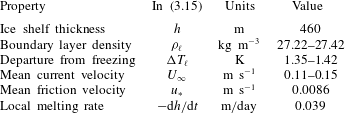
5.1 Ice thickness
Our heat balance for the ice–water interface can be integrated in time to model the evolution of ice thickness in the experiments conducted with (3.10) used for Phase 1 and (3.15) used for Phase 2. In what follows, the modelled ice thickness is denoted by
 $h_{m}$
. The values listed in table 2 for the properties of liquid water and solid ice are used in the integration.
$h_{m}$
. The values listed in table 2 for the properties of liquid water and solid ice are used in the integration.
 ${\rm\Delta}T_{s}$
and
${\rm\Delta}T_{s}$
and
 ${\rm\Delta}T_{\ell }$
in the heat balance are calculated in the following way:
${\rm\Delta}T_{\ell }$
in the heat balance are calculated in the following way:
 $$\begin{eqnarray}\displaystyle & \displaystyle {\rm\Delta}T_{s}=\left\{\begin{array}{@{}ll@{}}T_{f}-T_{A},\quad & \text{when ice is present,}\\ 0,\quad & \text{when there is no ice,}\end{array}\right. & \displaystyle\end{eqnarray}$$
 $$\begin{eqnarray}\displaystyle & \displaystyle {\rm\Delta}T_{\ell }=\left\{\begin{array}{@{}ll@{}}T_{G}-T_{f},\quad & \text{when ice is present,}\\ T_{G}-T_{A},\quad & \text{when there is no ice.}\end{array}\right. & \displaystyle\end{eqnarray}$$
 $T_{A}$
refers to temperature measurements at thermistor A, which is located in a small hole in the basal cooling plate, and
$T_{A}$
refers to temperature measurements at thermistor A, which is located in a small hole in the basal cooling plate, and
 $T_{G}$
refers to temperature measurements at thermistor G, which is located 5.25 cm above the basal cooling plate. The fluid velocity in the far field,
$T_{G}$
refers to temperature measurements at thermistor G, which is located 5.25 cm above the basal cooling plate. The fluid velocity in the far field,
 $U_{\infty }$
, is determined using the measurements of
$U_{\infty }$
, is determined using the measurements of
 $\overline{U_{{\it\theta}}}$
and
$\overline{U_{{\it\theta}}}$
and
 $\overline{U_{r}}$
interpolated at the angular velocity of the lid at a height
$\overline{U_{r}}$
interpolated at the angular velocity of the lid at a height
 $z=7$
cm:
$z=7$
cm:
 $$\begin{eqnarray}\displaystyle U_{\infty }=\sqrt{\overline{U_{{\it\theta}}(z)}^{2}+\overline{U_{r}(z)}^{2}},\quad z=7~\text{cm}. & & \displaystyle\end{eqnarray}$$
The friction velocity
 $u_{\ast }$
, which is used in calculating the coefficient of friction
$u_{\ast }$
, which is used in calculating the coefficient of friction
 $c_{f}$
defined in (3.14), is determined from the calibration shown in figure 13(b). The equations are integrated by a second-order Runge–Kutta method, with the initial condition for
$c_{f}$
defined in (3.14), is determined from the calibration shown in figure 13(b). The equations are integrated by a second-order Runge–Kutta method, with the initial condition for
 $h_{m}$
being zero. Because the temperature measurements were taken at intervals of 5 s, the time step for integration is also 5 s.
$h_{m}$
being zero. Because the temperature measurements were taken at intervals of 5 s, the time step for integration is also 5 s.

Figure 14. Misfit to (3.15) versus
 $G$
.
$G$
.

Figure 15. Comparison of
 $h_{e}$
(thinner solid line with shaded error region) with
$h_{e}$
(thinner solid line with shaded error region) with
 $h_{m}$
(thicker solid line) from (a) experiment 8, (b) experiment 5, (c) experiment 3 and (d) experiment 1. For
$h_{m}$
(thicker solid line) from (a) experiment 8, (b) experiment 5, (c) experiment 3 and (d) experiment 1. For
 $t<0$
, the error in
$t<0$
, the error in
 $h_{e}$
is 0.5 mm and for
$h_{e}$
is 0.5 mm and for
 $t>0$
, it is 0.9 mm. The hatched region in (c) is discussed in the text. For the
$t>0$
, it is 0.9 mm. The hatched region in (c) is discussed in the text. For the
 $h_{m}$
plots, the blue portion corresponds to ice thickness evolution in Phase 1 while the red portion corresponds ice thickness evolution in Phase 2.
$h_{m}$
plots, the blue portion corresponds to ice thickness evolution in Phase 1 while the red portion corresponds ice thickness evolution in Phase 2.
In Phase 2, the heat flux
 $q_{T}$
from the turbulent flow at the ice–water interface depends on the coefficient
$q_{T}$
from the turbulent flow at the ice–water interface depends on the coefficient
 $G$
. For the
$G$
. For the
 $Pr$
of water at 0 °C, which is listed in table 1,
$Pr$
of water at 0 °C, which is listed in table 1,
 $G$
becomes 62.7. We denote this value by
$G$
becomes 62.7. We denote this value by
 $G_{0}$
. The expression for
$G_{0}$
. The expression for
 $G$
is an empirical expression derived for a turbulent boundary layer in air over a perfectly flat plate (White Reference White1974). Using a range of values of
$G$
is an empirical expression derived for a turbulent boundary layer in air over a perfectly flat plate (White Reference White1974). Using a range of values of
 $G$
, including
$G$
, including
 $G_{0}$
, we evaluate
$G_{0}$
, we evaluate
 $h_{m}$
during Phase 2 of experiments 2–10. We also calculate the root mean square (r.m.s) difference
$h_{m}$
during Phase 2 of experiments 2–10. We also calculate the root mean square (r.m.s) difference
 ${\rm\Delta}h_{RMS}$
between
${\rm\Delta}h_{RMS}$
between
 $h_{e}$
and
$h_{e}$
and
 $h_{m}$
at the corresponding times. The omission of experiment 1 from this comparison will be explained when interpreting figure 15(d). The mean of
$h_{m}$
at the corresponding times. The omission of experiment 1 from this comparison will be explained when interpreting figure 15(d). The mean of
 ${\rm\Delta}h_{RMS}$
for the range of values of
${\rm\Delta}h_{RMS}$
for the range of values of
 $G$
considered is plotted in figure 14. Its minimum occurs when
$G$
considered is plotted in figure 14. Its minimum occurs when
 $G=36.0$
. The heat flux from the turbulent layer at the ice–water interface is therefore more closely approximated using this value of
$G=36.0$
. The heat flux from the turbulent layer at the ice–water interface is therefore more closely approximated using this value of
 $G$
, which will be denoted by
$G$
, which will be denoted by
 $G^{\prime }$
. The fact that
$G^{\prime }$
. The fact that
 $G^{\prime }$
is smaller than
$G^{\prime }$
is smaller than
 $G_{0}$
indicates that heat transfer from a turbulent flow at an ice–water interface is more efficient than at a flat plate. This enhanced heat transfer can be attributed to the ice surface not being uniformly smooth, especially during melting when it develops a wavy profile, since a rough surface has a greater surface area than a flat surface and hence allows for greater heat transfer. With the new value
$G_{0}$
indicates that heat transfer from a turbulent flow at an ice–water interface is more efficient than at a flat plate. This enhanced heat transfer can be attributed to the ice surface not being uniformly smooth, especially during melting when it develops a wavy profile, since a rough surface has a greater surface area than a flat surface and hence allows for greater heat transfer. With the new value
 $G^{\prime }$
, the heat transfer coefficient
$G^{\prime }$
, the heat transfer coefficient
 $C_{h}$
from the turbulent flow at the ice–water interface given in (3.12) is related to (
$C_{h}$
from the turbulent flow at the ice–water interface given in (3.12) is related to (
 $u_{\ast }/U_{\infty }$
) by the power law
$u_{\ast }/U_{\infty }$
) by the power law
 $C_{h}=0.028(u_{\ast }/U_{\infty })^{1.09}$
.
$C_{h}=0.028(u_{\ast }/U_{\infty })^{1.09}$
.

Figure 16. Contour plot of
 $h_{m}$
for
$h_{m}$
for
 $Re_{R}$
corresponding to experiments 2–10. The white line represents the onset of turbulent mixing, the dashed vertical black lines indicate the
$Re_{R}$
corresponding to experiments 2–10. The white line represents the onset of turbulent mixing, the dashed vertical black lines indicate the
 $Re_{R}$
of the experiments, and the contour plot is filled by linearly interpolating modelled ice thickness values at the distinct
$Re_{R}$
of the experiments, and the contour plot is filled by linearly interpolating modelled ice thickness values at the distinct
 $Re_{R}$
of the experiments.
$Re_{R}$
of the experiments.
 $G^{\prime }$
is substituted in (3.15) to calculate
$G^{\prime }$
is substituted in (3.15) to calculate
 $h_{m}$
for Phase 2 of experiments 1–10. Figure 15 shows the comparison between
$h_{m}$
for Phase 2 of experiments 1–10. Figure 15 shows the comparison between
 $h_{e}$
and
$h_{e}$
and
 $h_{m}$
in experiments 8, 5, 3 and 1. There is good agreement between
$h_{m}$
in experiments 8, 5, 3 and 1. There is good agreement between
 $h_{e}$
and
$h_{e}$
and
 $h_{m}$
in experiments 8, 5 and 3 but not in Phase 2 of experiment 1. After the onset of turbulent mixing in experiment 1, a stratified layer remained between the turbulent layer and the ice–water interface up to
$h_{m}$
in experiments 8, 5 and 3 but not in Phase 2 of experiment 1. After the onset of turbulent mixing in experiment 1, a stratified layer remained between the turbulent layer and the ice–water interface up to
 $t=33$
min. This was evidenced by the behaviour of dye inserted into the turbulent layer, which showed that a clear, stratified layer over the ice–water interface prevented the dyed turbulent layer from reaching the ice surface. Accordingly, the ice growth in that time interval is modelled using (3.10). For this case, the measured rate of ice growth is larger than predicted, a difference which occurs because the stratified layer over the ice–water interface inhibits heat transfer from the liquid far field. Ice grows below the turbulent layer from
$t=33$
min. This was evidenced by the behaviour of dye inserted into the turbulent layer, which showed that a clear, stratified layer over the ice–water interface prevented the dyed turbulent layer from reaching the ice surface. Accordingly, the ice growth in that time interval is modelled using (3.10). For this case, the measured rate of ice growth is larger than predicted, a difference which occurs because the stratified layer over the ice–water interface inhibits heat transfer from the liquid far field. Ice grows below the turbulent layer from
 $t=0$
to
$t=0$
to
 $t=33$
min, at which time it reaches the turbulence. For
$t=33$
min, at which time it reaches the turbulence. For
 $t>33$
min,
$t>33$
min,
 $h_{m}$
is modelled using (3.15). The model predicts melting whereas the experimental measurements indicate attenuated growth. The disagreement between
$h_{m}$
is modelled using (3.15). The model predicts melting whereas the experimental measurements indicate attenuated growth. The disagreement between
 $h_{e}$
and
$h_{e}$
and
 $h_{m}$
in experiment 1 reveals a limitation of our model. At the lower end of the range of
$h_{m}$
in experiment 1 reveals a limitation of our model. At the lower end of the range of
 $Re_{R}$
we investigate, the applied shear stress from the lid is low, and consequently the turbulence is too weak to erode the stratified layer quickly. Our model, however, assumes that the stratified layer becomes eroded quickly at low values of
$Re_{R}$
we investigate, the applied shear stress from the lid is low, and consequently the turbulence is too weak to erode the stratified layer quickly. Our model, however, assumes that the stratified layer becomes eroded quickly at low values of
 $Re_{R}$
.
$Re_{R}$
.

Figure 17. Contour plot of absolute difference between
 $h_{e}$
and
$h_{e}$
and
 $h_{m}$
for experiments 2–10. The distinct
$h_{m}$
for experiments 2–10. The distinct
 $Re_{R}$
of the experiments are marked by the dashed vertical black lines. Data corresponding to the
$Re_{R}$
of the experiments are marked by the dashed vertical black lines. Data corresponding to the
 $Re_{R}$
of the experiments are linearly interpolated to make the contour plot.
$Re_{R}$
of the experiments are linearly interpolated to make the contour plot.
A stratified layer is present in experiments 2–4 for a short time interval following the onset of turbulent mixing. Although the theoretical model given by (3.10) is incomplete for this configuration, we use it to approximate
 $h_{m}$
until the time when the turbulent layer comes into contact with the ice.
$h_{m}$
until the time when the turbulent layer comes into contact with the ice.
 $h_{m}$
is consistently lower than
$h_{m}$
is consistently lower than
 $h_{e}$
in that time interval, as shown in the hatched region of figure 15(c) for experiment 3. In the determination of
$h_{e}$
in that time interval, as shown in the hatched region of figure 15(c) for experiment 3. In the determination of
 $G^{\prime }$
previously discussed,
$G^{\prime }$
previously discussed,
 $h_{e}$
and
$h_{e}$
and
 $h_{m}$
from time intervals when a stratified layer was present were not used.
$h_{m}$
from time intervals when a stratified layer was present were not used.
The contour plot of
 $h_{m}$
calculated using the theoretical model with
$h_{m}$
calculated using the theoretical model with
 $G^{\prime }$
for experiments 2–10 is shown in figure 16. Experiment 1 is omitted because it is a case for which our model is not valid. The region corresponding to experiment 1 in figure 16 is hatched. The absolute difference between
$G^{\prime }$
for experiments 2–10 is shown in figure 16. Experiment 1 is omitted because it is a case for which our model is not valid. The region corresponding to experiment 1 in figure 16 is hatched. The absolute difference between
 $h_{e}$
from figure 5 and
$h_{e}$
from figure 5 and
 $h_{m}$
at corresponding times is shown in figure 17. The absolute difference is generally close to the error margin of 0.5 mm for Phase 1 and 0.9 mm for Phase 2, which indicates good agreement between the model and the experiment. The hatched area in figure 17 corresponds to experiment 1 and time intervals when a stratified layer was present during Phase 2 of the experiments. The absolute difference between
$h_{m}$
at corresponding times is shown in figure 17. The absolute difference is generally close to the error margin of 0.5 mm for Phase 1 and 0.9 mm for Phase 2, which indicates good agreement between the model and the experiment. The hatched area in figure 17 corresponds to experiment 1 and time intervals when a stratified layer was present during Phase 2 of the experiments. The absolute difference between
 $h_{e}$
and
$h_{e}$
and
 $h_{m}$
in these intervals during Phase 2 was omitted from the contour plot because the model assumes that the stratified layer is eroded more rapidly and hence deviates from the experimental measurements.
$h_{m}$
in these intervals during Phase 2 was omitted from the contour plot because the model assumes that the stratified layer is eroded more rapidly and hence deviates from the experimental measurements.
We did not observe evidence of the radial component of the flow near the bottom of the tank during turbulent mixing affecting the evolution of ice in our set of experiments. The radial component of the flow is stronger at higher
 $Re_{R}$
. In all experiments in which there is transient melting, the rate at which the ice melts always increases with distance from the centre of the tank. During the subsequent refreezing, the rate of ice growth is always uniform at all radial distances. These observations suggest that the far-field flow has a stronger influence on the evolution of ice than the radial flow near the bottom of the tank.
$Re_{R}$
. In all experiments in which there is transient melting, the rate at which the ice melts always increases with distance from the centre of the tank. During the subsequent refreezing, the rate of ice growth is always uniform at all radial distances. These observations suggest that the far-field flow has a stronger influence on the evolution of ice than the radial flow near the bottom of the tank.
6 Discussion
6.1 Application to observations under Pine Island Glacier Ice Shelf
Pine Island Glacier Ice Shelf is a 40 km long, 20 km wide ice shelf in the Amundsen Sea off West Antarctica. An investigation involving the deployment of autonomous underwater vehicles in its underlying ocean cavity showed that the basal surface of the ice shelf is experiencing rapid melting, probably due to shoaling Circumpolar Deep Water and intrusion of warmer water under the ice (Jenkins et al. Reference Jenkins, Dutrieux, Jacobs, McPhail, Perrett, Webb and White2010a ).
Stanton et al. (Reference Stanton, Shaw, Truffer, Corr, Peters, Riverman, Bindschadler, Holland and Anandakrishnan2013) reported in situ measurements of the basal melt rate and ocean boundary layer properties from a site in the centre of Pine Island Glacier Ice Shelf where a hole was drilled vertically from the surface to access the water underneath. We use the measurements, which are listed in table 4, to test our heat transfer model from (3.15) with
 $G=G^{\prime }$
. The boundary layer depth and density at the site were obtained from conductivity–temperature–depth (CTD) profiling. The departure from freezing, mean current velocity, mean friction velocity and local melting rate were measured using a flux package installed at an initial distance of 2.3 m below the ice shelf base. The range of values listed for the departure from freezing and mean current velocity are for a 35 day period. The mean friction velocity was constant in that period. The local melt rate is from a fit through measurements from days 5–35 and is equivalent to 14
$G=G^{\prime }$
. The boundary layer depth and density at the site were obtained from conductivity–temperature–depth (CTD) profiling. The departure from freezing, mean current velocity, mean friction velocity and local melting rate were measured using a flux package installed at an initial distance of 2.3 m below the ice shelf base. The range of values listed for the departure from freezing and mean current velocity are for a 35 day period. The mean friction velocity was constant in that period. The local melt rate is from a fit through measurements from days 5–35 and is equivalent to 14
 $\text{m}~\text{yr}^{-1}$
. We substitute
$\text{m}~\text{yr}^{-1}$
. We substitute
 $h$
,
$h$
,
 $u_{\ast }$
, and the medians of the range of values of
$u_{\ast }$
, and the medians of the range of values of
 ${\it\rho}_{\ell }$
,
${\it\rho}_{\ell }$
,
 ${\rm\Delta}T_{\ell }$
and
${\rm\Delta}T_{\ell }$
and
 $U_{\infty }$
from table 4,
$U_{\infty }$
from table 4,
 ${\it\rho}_{s}$
,
${\it\rho}_{s}$
,
 $k_{s}$
and
$k_{s}$
and
 $L$
from table 2, a typical value of
$L$
from table 2, a typical value of
 $c_{\ell }=4.00\times 10^{3}~\text{J}~\text{kg}^{-1}~\text{K}^{-1}$
for sea water and a typical value of
$c_{\ell }=4.00\times 10^{3}~\text{J}~\text{kg}^{-1}~\text{K}^{-1}$
for sea water and a typical value of
 ${\rm\Delta}T_{s}=19$
K (Tyler et al.
Reference Tyler, Holland, Zagorodnov, Stern, Sladek, Kobs, White, Suárez and Bryenton2013) for an Antarctic ice shelf in (3.15). This yields a predicted melt rate
${\rm\Delta}T_{s}=19$
K (Tyler et al.
Reference Tyler, Holland, Zagorodnov, Stern, Sladek, Kobs, White, Suárez and Bryenton2013) for an Antarctic ice shelf in (3.15). This yields a predicted melt rate
 $-\text{d}h/\text{d}t$
of 98
$-\text{d}h/\text{d}t$
of 98
 $\text{m}~\text{yr}^{-1}$
.
$\text{m}~\text{yr}^{-1}$
.
Table 4. Measurements of the ocean boundary layer properties from Stanton et al. (Reference Stanton, Shaw, Truffer, Corr, Peters, Riverman, Bindschadler, Holland and Anandakrishnan2013).

The fact that our model over-predicts the observed melt rate can be partly explained by the observed
 ${\rm\Delta}T_{\ell }$
being across a thick stable stratified boundary layer. Our model is not valid for the interaction of a stable stratified layer with an ice–water interface. Eddy diffusivity in a stratified turbulent flow is lower than in an unstratified turbulent flow (Galperin, Sukoriansky & Anderson Reference Galperin, Sukoriansky and Anderson2007), which can account partly for the discrepancy between the observed and modelled melt rates. Our predicted value of the melt rate at the measurement site is an upper limit and corresponds to the case where a well-mixed turbulent warm water flow comes in direct contact with the ice–water interface.
${\rm\Delta}T_{\ell }$
being across a thick stable stratified boundary layer. Our model is not valid for the interaction of a stable stratified layer with an ice–water interface. Eddy diffusivity in a stratified turbulent flow is lower than in an unstratified turbulent flow (Galperin, Sukoriansky & Anderson Reference Galperin, Sukoriansky and Anderson2007), which can account partly for the discrepancy between the observed and modelled melt rates. Our predicted value of the melt rate at the measurement site is an upper limit and corresponds to the case where a well-mixed turbulent warm water flow comes in direct contact with the ice–water interface.
In this application, phase change due to heat transfer through the boundary layer only is considered. The transfer of salt through the boundary layer is ignored. A mean vertical salt flux of
 $2.8\times 10^{-6}~\text{psu ms}^{-1}$
was also measured at the observation site by Stanton et al. (Reference Stanton, Shaw, Truffer, Corr, Peters, Riverman, Bindschadler, Holland and Anandakrishnan2013). Both the conservation of heat and the conservation of salt at the interface control the rate of phase change. Whether heat transfer or salt transfer is the more dominant effect in causing the phase change at this site remains an open question. A complete analysis should consider both effects, and include data from different levels within the boundary layer.
$2.8\times 10^{-6}~\text{psu ms}^{-1}$
was also measured at the observation site by Stanton et al. (Reference Stanton, Shaw, Truffer, Corr, Peters, Riverman, Bindschadler, Holland and Anandakrishnan2013). Both the conservation of heat and the conservation of salt at the interface control the rate of phase change. Whether heat transfer or salt transfer is the more dominant effect in causing the phase change at this site remains an open question. A complete analysis should consider both effects, and include data from different levels within the boundary layer.
6.2 Comparison of
 ${\it\gamma}_{T}$
from our model with other expressions for
${\it\gamma}_{T}$
${\it\gamma}_{T}$
from our model with other expressions for
${\it\gamma}_{T}$


The parameterization of the thermal exchange velocity across the boundary layer in our model is
 $$\begin{eqnarray}\displaystyle {\it\gamma}_{T}=U_{\infty }C_{h}=U_{\infty }\left(\frac{c_{f}/2}{1+G^{\prime }\sqrt{c_{f}/2}}\right). & & \displaystyle\end{eqnarray}$$
This parameterization is compared against two formulations used in the literature. Jenkins (Reference Jenkins1991) expressed
 ${\it\gamma}_{T}$
as
${\it\gamma}_{T}$
as
 $$\begin{eqnarray}\displaystyle {\it\gamma}_{T}=\frac{C_{d}^{1/2}U_{\infty }}{2.12\ln (C_{d}^{1/2}Re)+12.5Pr^{2/3}-8.68}, & & \displaystyle\end{eqnarray}$$
where
 $C_{d}$
is a dimensionless drag coefficient given by
$C_{d}$
is a dimensionless drag coefficient given by
 $$\begin{eqnarray}\displaystyle C_{d}=\frac{u_{\ast }^{2}}{U_{\infty }^{2}}. & & \displaystyle\end{eqnarray}$$
The expressions (6.1) and (6.2) for
 ${\it\gamma}_{T}$
are essentially equivalent, being related by the Prandtl–Nikuradse skin friction law (Kader & Yaglom Reference Kader and Yaglom1972). A constant Stanton number
${\it\gamma}_{T}$
are essentially equivalent, being related by the Prandtl–Nikuradse skin friction law (Kader & Yaglom Reference Kader and Yaglom1972). A constant Stanton number
 $C_{h}$
is used by Jenkins (Reference Jenkins2011) for heat transfer through the boundary layer. This is converted to the thermal exchange velocity
$C_{h}$
is used by Jenkins (Reference Jenkins2011) for heat transfer through the boundary layer. This is converted to the thermal exchange velocity
 ${\it\gamma}_{T}$
using
${\it\gamma}_{T}$
using
 ${\it\gamma}_{T}=U_{\infty }C_{h}$
. The values of
${\it\gamma}_{T}=U_{\infty }C_{h}$
. The values of
 ${\it\gamma}_{T}$
calculated from (6.1), (6.2) and the constant Stanton number of Jenkins (Reference Jenkins2011) for the range of friction velocities covered by experiment 2–10 are compared in figure 18. For the configuration where a warm turbulent layer is in direct contact with an ice surface, our experimentally constrained model estimates that the thermal exchange velocity is larger than conventional models assume.
${\it\gamma}_{T}$
calculated from (6.1), (6.2) and the constant Stanton number of Jenkins (Reference Jenkins2011) for the range of friction velocities covered by experiment 2–10 are compared in figure 18. For the configuration where a warm turbulent layer is in direct contact with an ice surface, our experimentally constrained model estimates that the thermal exchange velocity is larger than conventional models assume.

Figure 18. Thermal exchange velocity
 ${\it\gamma}_{T}$
corresponding to the
${\it\gamma}_{T}$
corresponding to the
 $u_{\ast }$
from our experiments:
$u_{\ast }$
from our experiments:
 $\ast$
from (6.1), ▵ from (6.2) and ▫ from Jenkins (Reference Jenkins2011).
$\ast$
from (6.1), ▵ from (6.2) and ▫ from Jenkins (Reference Jenkins2011).
7 Summary
We have conducted experiments on the melting of ice in a turbulent shear flow that transports warm water to the ice–water interface. A modified heat transfer law, originally derived for turbulent flow over a flat plate and which depends on the friction velocity of the flow, allows us to model the evolution of the ice thickness correctly. Our experiments have dynamic similarity with the geophysical system of the ocean cavity beneath an ice shelf through the Rossby number and thermodynamic similarity through the Stefan number. Although our experiments do not include the effect of salinity, they reveal the mechanisms through which warm water transport to an ice shelf’s basal surface accelerates basal melting. Through this study, we propose an experimentally constrained expression for the thermal exchange velocity
 ${\it\gamma}_{T}$
in ice–ocean interaction.
${\it\gamma}_{T}$
in ice–ocean interaction.
Acknowledgements
We thank Y. Li and H. Chen for help in conducting the PIV measurements. We also thank X. I. A. Yang for helpful discussion. The experiments were financially supported by NSF grant EAR-110371.