


1 Introduction
In many industrial processes that involve heat transfer and turbulent flows, significant temperature (or pressure) gradients can lead to large thermophysical property variations. This is especially the case when fluids at supercritical pressure are heated or cooled across the pseudo-critical point. Heated or cooled fluids at such pressures can be found in refrigeration applications, during fuel combustion in rocket engines and in supercritical power cycles. When a fluid at supercritical pressure is heated, it transitions from a fluid with liquid-like properties to a fluid with gas-like properties. The temperature about which this transition occurs is called the pseudo-critical temperature
 $T_{pc}$
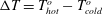
, which is defined as the temperature for which the specific heat capacity has its maximum value. Close to the pseudo-critical temperature, the thermophysical properties vary sharply with temperature, as is shown in figure 1.
$T_{pc}$
, which is defined as the temperature for which the specific heat capacity has its maximum value. Close to the pseudo-critical temperature, the thermophysical properties vary sharply with temperature, as is shown in figure 1.

Figure 1. Non-dimensionalized thermophysical properties of carbon dioxide at 8 MPa as a function of non-dimensional temperature;
 $T_{pc}=307.7$
K. The properties have been obtained from the equation of state by Kunz, Klimeck & Jaeschke (Reference Kunz, Klimeck, Wagner and Jaeschke2007) and equations from Fenghour, Wakeham & Vesovic (Reference Fenghour, Wakeham and Vesovic1998) and Vesovic et al. (Reference Vesovic, Wakeham, Olchowy, Sengers, Watson and Millat1990). The properties have been non-dimensionalized such that they vary around unity, purely for illustrative purposes. The horizontal axis represents a temperature difference of 12 K.
$T_{pc}=307.7$
K. The properties have been obtained from the equation of state by Kunz, Klimeck & Jaeschke (Reference Kunz, Klimeck, Wagner and Jaeschke2007) and equations from Fenghour, Wakeham & Vesovic (Reference Fenghour, Wakeham and Vesovic1998) and Vesovic et al. (Reference Vesovic, Wakeham, Olchowy, Sengers, Watson and Millat1990). The properties have been non-dimensionalized such that they vary around unity, purely for illustrative purposes. The horizontal axis represents a temperature difference of 12 K.
It is known that the thermophysical property variations that occur in heated turbulent fluids at supercritical pressure may lead to relaminarization of the flow, which will result in deteriorated heat transfer. Kurganov & Kaptil’ny (Reference Kurganov and Kaptil’ny1992) associated the deteriorated heat transfer with changes in the velocity and shear stress profiles, which occur as a consequence of buoyancy forces in flows with a mean negative pressure gradient (mixed convection flows). However, heat transfer deterioration may also occur as a result of acceleration of the bulk flow with negligible buoyancy effects (see e.g. Shiralkar & Griffith Reference Shiralkar and Griffith1970; Jackson Reference Jackson2013). Yoo (Reference Yoo2013) extensively reviewed heat transfer to fluids at supercritical pressure. That review showed that it is difficult (if not impossible) to predict heat transfer deterioration in fluids at supercritical pressure accurately while using turbulence modelling or Nusselt-number relations.
In order to understand how the thermophysical property variations of a fluid at supercritical pressure affect heat transfer, it is important to understand how the flow, and turbulence in particular, are affected by thermophysical property variations. This is not yet fully understood. However, such knowledge will help in the design of better heat transfer models, such as Nusselt-number relations and turbulence models.
To investigate the effect of thermophysical property variations on turbulent flow characteristics, Bae, Yoo & Choi (Reference Bae, Yoo and Choi2005) and Bae, Yoo & McEligot (Reference Bae, Yoo and McEligot2008) simulated heat transfer to supercritical carbon dioxide (
 $\text{sCO}_{2}$
) at 8 MPa in a pipe and annular geometry, respectively. Bae et al. (Reference Bae, Yoo and Choi2005) reported significantly decreased vortical motions near the heated surface. This is an important observation, as streamwise vortices are an integral part of the self-regenerating process of near-wall turbulence (see e.g. Hamilton, Kim & Waleffe Reference Hamilton, Kim and Waleffe1995; Waleffe Reference Waleffe1997). Bae et al. (Reference Bae, Yoo and McEligot2008) found that velocity profiles and shear stress profiles are significantly affected by acceleration and the combined effect of buoyancy and a negative streamwise pressure gradient; such findings are qualitatively in line with the experiments by Kurganov & Kaptil’ny (Reference Kurganov and Kaptil’ny1992).
$\text{sCO}_{2}$
) at 8 MPa in a pipe and annular geometry, respectively. Bae et al. (Reference Bae, Yoo and Choi2005) reported significantly decreased vortical motions near the heated surface. This is an important observation, as streamwise vortices are an integral part of the self-regenerating process of near-wall turbulence (see e.g. Hamilton, Kim & Waleffe Reference Hamilton, Kim and Waleffe1995; Waleffe Reference Waleffe1997). Bae et al. (Reference Bae, Yoo and McEligot2008) found that velocity profiles and shear stress profiles are significantly affected by acceleration and the combined effect of buoyancy and a negative streamwise pressure gradient; such findings are qualitatively in line with the experiments by Kurganov & Kaptil’ny (Reference Kurganov and Kaptil’ny1992).
More recently, Zonta, Marchioli & Soldati (Reference Zonta, Marchioli and Soldati2012) and Lee et al. (Reference Lee, Jung, Sung and Zaki2013) showed the effect of variable dynamic viscosity, representative of a fluid at subcritical pressure, on a channel flow and a boundary layer flow. They found that the variation in viscosity causes the turbulence intensities to diminish. More specifically, Zonta et al. (Reference Zonta, Marchioli and Soldati2012) report that the streak characteristics are altered due to the variation in viscosity. Strong variations of dynamic viscosity and thermal expansion coefficient were shown to have a large impact on momentum and heat transfer in stably stratified channel flows (Zonta, Marchioli & Soldati Reference Zonta, Marchioli and Soldati2012; Zonta Reference Zonta2013). High-viscosity regions dampen the turbulent intensities, whereas low-viscosity regions enhance the intensities. In the same study, a temperature-dependent thermal expansion coefficient was found to have the opposite effect. Unstable density stratification in a horizontal channel flow configuration was found to significantly increase momentum and heat transfer by Zonta & Soldati (Reference Zonta and Soldati2014). These studies show that the nonlinear thermophysical property relations for the thermophysical properties (non-Oberbeck–Boussinesq conditions) may have a profound effect on flow statistics and flow structures. It is also interesting to note here that Patel et al. (Reference Patel, Peeters, Boersma and Pecnik2015) found that the stability of streaks is significantly affected by mean density and viscosity stratification. These findings are important, as streaks not only contribute greatly to the turbulent shear stress (Willmarth & Lu Reference Willmarth and Lu1972), but also are an integral part of the self-regenerating process of near-wall turbulence.
In this paper, we will investigate how the variable thermophysical properties of a heated (or cooled) fluid at supercritical pressure affect turbulent motions in a qualitative as well as a quantitative manner. Firstly, we are interested in what the influence of a mean density and dynamic viscosity variation is on the flow field. Secondly, we would like to investigate how instantaneous density and dynamic viscosity fluctuations affect the turbulent motions, and, more specifically, turbulent structures such as the near-wall streaks and streamwise vortices, which are important to the self-regeneration of turbulence in the near-wall region. Lastly, we want to investigate the role of variable Prandtl number with respect to the generation of turbulent structures, as it determines the magnitude of the thermal fluctuations and therefore the thermophysical property fluctuations.
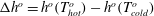
To this end, we will show results from direct numerical simulations (DNS) of simultaneously heated and cooled turbulent supercritical fluids flowing upwards in an annular geometry at a Reynolds number of 8000. A schematic of the investigated geometry is shown in figure 2. The temperature crosses the pseudo-critical point within the flow field. The inner wall of the annular geometry is kept at a high temperature, while the outer wall is kept at a low temperature. In this manner, a statistically fully developed temperature and flow profile can be obtained. This allows us to focus on local variable thermophysical properties effects on turbulence, because effects such as a growing thermal boundary layer and mean streamwise flow acceleration will not be present.

Figure 2. The annular geometry of the simulations. The inner and outer wall radii (
 $R_{in}$
and
$R_{in}$
and
 $R_{out}$
), the length
$R_{out}$
), the length
 $L$
and the inner and outer wall temperatures (
$L$
and the inner and outer wall temperatures (
 $T_{hot}$
and
$T_{hot}$
and
 $T_{cold}$
) are shown.
$T_{cold}$
) are shown.
The governing equations and numerical methods of the DNS are presented in § 2. In § 3, we will discuss the effect of the mean density and viscosity profiles of supercritical carbon dioxide (
 $\text{sCO}_{2}$
) on mean flow statistics first. Thereafter we will show the influence of the instantaneous density and dynamic viscosity variations on turbulent structures. Finally, we present a summary of the most important conclusions in § 4. At the end of this work, three appendices can be found. In appendix A, mesh generation and enthalpy power spectra are presented. In appendix B, numerical code validations are shown. Appendix C outlines several derivations that are used in this work.
$\text{sCO}_{2}$
) on mean flow statistics first. Thereafter we will show the influence of the instantaneous density and dynamic viscosity variations on turbulent structures. Finally, we present a summary of the most important conclusions in § 4. At the end of this work, three appendices can be found. In appendix A, mesh generation and enthalpy power spectra are presented. In appendix B, numerical code validations are shown. Appendix C outlines several derivations that are used in this work.
2 Computational details
2.1 Governing equations
We assume that the heated supercritical
 $\text{CO}_{2}$
flow under investigation may be considered to be in local thermodynamic equilibrium. This assumption is valid for length scales
$\text{CO}_{2}$
flow under investigation may be considered to be in local thermodynamic equilibrium. This assumption is valid for length scales
 ${\it\Lambda}$
that are larger than the correlation length scale
${\it\Lambda}$
that are larger than the correlation length scale
 ${\it\xi}$
that is associated with density fluctuations that arise due to variations in the number of molecules in a given volume. Under the assumption that
${\it\xi}$
that is associated with density fluctuations that arise due to variations in the number of molecules in a given volume. Under the assumption that
 ${\it\Lambda}>{\it\xi}$
, the fluid state is described by the hydrodynamic conservation equations for a low-Mach-number fluid (Zappoli, Beysens & Garrabos Reference Zappoli, Beysens and Garrabos2015). Experiments that were performed by Nishikawa & Tanaka (Reference Nishikawa and Tanaka1995) in order to calculate
${\it\Lambda}>{\it\xi}$
, the fluid state is described by the hydrodynamic conservation equations for a low-Mach-number fluid (Zappoli, Beysens & Garrabos Reference Zappoli, Beysens and Garrabos2015). Experiments that were performed by Nishikawa & Tanaka (Reference Nishikawa and Tanaka1995) in order to calculate
 ${\it\xi}$
in supercritical
${\it\xi}$
in supercritical
 $\text{CO}_{2}$
suggest that this assumption is reasonable. Furthermore, we aim to investigate heated supercritical
$\text{CO}_{2}$
suggest that this assumption is reasonable. Furthermore, we aim to investigate heated supercritical
 $\text{CO}_{2}$
flows at 8 MPa, which is substantially higher than the pressure at the critical point (7.4 MPa). Therefore, the low-Mach-number approximation of the Navier–Stokes equations is numerically solved to simulate heated and/or cooled flows at supercritical pressure in cylindrical geometries. The low-Mach-number approximation has previously been used to simulate such flows by Bae et al. (Reference Bae, Yoo and Choi2005, Reference Bae, Yoo and McEligot2008), Nemati et al. (Reference Nemati, Patel, Boersma and Pecnik2015) and Patel et al. (Reference Patel, Peeters, Boersma and Pecnik2015). In the low-Mach-number limit of the Navier–Stokes equations, the effect of acoustic waves on the solution is neglected. The pressure is decomposed into a thermodynamic part
$\text{CO}_{2}$
flows at 8 MPa, which is substantially higher than the pressure at the critical point (7.4 MPa). Therefore, the low-Mach-number approximation of the Navier–Stokes equations is numerically solved to simulate heated and/or cooled flows at supercritical pressure in cylindrical geometries. The low-Mach-number approximation has previously been used to simulate such flows by Bae et al. (Reference Bae, Yoo and Choi2005, Reference Bae, Yoo and McEligot2008), Nemati et al. (Reference Nemati, Patel, Boersma and Pecnik2015) and Patel et al. (Reference Patel, Peeters, Boersma and Pecnik2015). In the low-Mach-number limit of the Navier–Stokes equations, the effect of acoustic waves on the solution is neglected. The pressure is decomposed into a thermodynamic part
 $p_{0}(t)$
and a hydrodynamic part
$p_{0}(t)$
and a hydrodynamic part
 $p_{hy}(t)$
. The fluctuations of the hydrodynamic pressure are assumed to be very small compared to the thermodynamic pressure, so that all thermophysical property variations due to hydrodynamic pressure fluctuations can be neglected. Therefore, all thermophysical properties can be evaluated as a function of the enthalpy only. Well above the critical pressure, the speed of sound shows a minimum at the pseudo-critical temperature. For
$p_{hy}(t)$
. The fluctuations of the hydrodynamic pressure are assumed to be very small compared to the thermodynamic pressure, so that all thermophysical property variations due to hydrodynamic pressure fluctuations can be neglected. Therefore, all thermophysical properties can be evaluated as a function of the enthalpy only. Well above the critical pressure, the speed of sound shows a minimum at the pseudo-critical temperature. For
 $\text{sCO}_{2}$
at 8 MPa, the minimum value of the speed of sound is
$\text{sCO}_{2}$
at 8 MPa, the minimum value of the speed of sound is
 $179~\text{m}~\text{s}^{-1}$
. Thus when considering bulk velocities of
$179~\text{m}~\text{s}^{-1}$
. Thus when considering bulk velocities of
 $1~\text{m}~\text{s}^{-1}$
, the Mach number is even less than 0.01, which validates the use of the low-Mach-number approximation.
$1~\text{m}~\text{s}^{-1}$
, the Mach number is even less than 0.01, which validates the use of the low-Mach-number approximation.
Using dyadic notation and denoting a vector with a bold symbol, while denoting a second-order tensor with a capital bold symbol, the governing equations for conservation of mass, momentum and enthalpy in non-dimensional form read
 $$\begin{eqnarray}\partial _{t}{\it\rho}+\boldsymbol{{\rm\nabla}}\boldsymbol{\cdot }{\it\rho}\boldsymbol{u}=0,\end{eqnarray}$$
 $$\begin{eqnarray}\partial _{t}({\it\rho}\boldsymbol{u})+\boldsymbol{{\rm\nabla}}\boldsymbol{\cdot }({\it\rho}\boldsymbol{u}\boldsymbol{u})=-\boldsymbol{{\rm\nabla}}p_{hy}+Fr^{-1}{\it\rho}\hat{\boldsymbol{z}}+Re^{-1}\boldsymbol{{\rm\nabla}}\boldsymbol{\cdot }2{\it\mu}\unicode[STIX]{x1D64E},\end{eqnarray}$$
where
 $$\begin{eqnarray}\unicode[STIX]{x1D64E}\equiv {\textstyle \frac{1}{2}}(\boldsymbol{{\rm\nabla}}\boldsymbol{u}+(\boldsymbol{{\rm\nabla}}\boldsymbol{u})^{\text{T}})-{\textstyle \frac{1}{3}}(\boldsymbol{{\rm\nabla}}\boldsymbol{\cdot }\boldsymbol{u})\unicode[STIX]{x1D644}\end{eqnarray}$$
and
 $$\begin{eqnarray}\partial _{t}({\it\rho}h)+\boldsymbol{{\rm\nabla}}\boldsymbol{\cdot }{\it\rho}\boldsymbol{u}h=(Re\,Pr_{h})^{-1}\boldsymbol{{\rm\nabla}}\boldsymbol{\cdot }k\boldsymbol{{\rm\nabla}}T,\end{eqnarray}$$
in which
 ${\it\rho}$
is the density,
${\it\rho}$
is the density,
 $\boldsymbol{u}$
the velocity,
$\boldsymbol{u}$
the velocity,
 $Fr$
the Froude number,
$Fr$
the Froude number,
 $\hat{\boldsymbol{z}}$
the streamwise unit vector,
$\hat{\boldsymbol{z}}$
the streamwise unit vector,
 $Re$
the Reynolds number,
$Re$
the Reynolds number,
 ${\it\mu}$
the dynamic viscosity,
${\it\mu}$
the dynamic viscosity,
 $\unicode[STIX]{x1D64E}$
the deviatoric stress tensor,
$\unicode[STIX]{x1D64E}$
the deviatoric stress tensor,
 $\unicode[STIX]{x1D644}$
the identity tensor,
$\unicode[STIX]{x1D644}$
the identity tensor,
 $h$
the enthalpy,
$h$
the enthalpy,
 $Pr_{h}$
the reference Prandtl number based on a ratio of an enthalpy difference and a temperature difference,
$Pr_{h}$
the reference Prandtl number based on a ratio of an enthalpy difference and a temperature difference,
 $k$
the thermal conductivity and
$k$
the thermal conductivity and
 $T$
the temperature. All variables in the equations presented above are scaled with bulk quantities, i.e. the spatial coordinates are scaled with the hydraulic diameter
$T$
the temperature. All variables in the equations presented above are scaled with bulk quantities, i.e. the spatial coordinates are scaled with the hydraulic diameter
 $D_{h}^{o}$
, the velocity with the bulk streamwise velocity
$D_{h}^{o}$
, the velocity with the bulk streamwise velocity
 $w_{b}^{o}$
, and the time with
$w_{b}^{o}$
, and the time with
 $D_{h}^{o}/w_{b}^{o}$
. The superscript
$D_{h}^{o}/w_{b}^{o}$
. The superscript
 $^{o}$
denotes a dimensional quantity. All thermophysical properties were scaled with their respective values at the pseudo-critical point, i.e.
$^{o}$
denotes a dimensional quantity. All thermophysical properties were scaled with their respective values at the pseudo-critical point, i.e.
 ${\it\rho}={\it\rho}^{o}/{\it\rho}_{pc}^{o}$
and
${\it\rho}={\it\rho}^{o}/{\it\rho}_{pc}^{o}$
and
 ${\it\mu}={\it\mu}^{o}/{\it\mu}_{pc}^{o}$
, where the subscript
${\it\mu}={\it\mu}^{o}/{\it\mu}_{pc}^{o}$
, where the subscript
 $pc$
denotes a property at the pseudo-critical temperature. The hydrodynamic pressure is therefore scaled with
$pc$
denotes a property at the pseudo-critical temperature. The hydrodynamic pressure is therefore scaled with
 ${\it\rho}_{pc}^{o}{w_{b}^{o}}^{2}$
. Both the enthalpy and the temperature have been non-dimensionalized such that
${\it\rho}_{pc}^{o}{w_{b}^{o}}^{2}$
. Both the enthalpy and the temperature have been non-dimensionalized such that
 $0\leqslant h\leqslant 1$
and
$0\leqslant h\leqslant 1$
and
 $0\leqslant T\leqslant 1$
, i.e.
$0\leqslant T\leqslant 1$
, i.e.
 $$\begin{eqnarray}h=\frac{h^{o}-h_{cold}^{o}}{{\rm\Delta}h^{o}},\quad T=\frac{T^{o}-T_{cold}^{o}}{{\rm\Delta}T^{o}},\end{eqnarray}$$
where
 $T_{cold}^{o}$
represents the lowest possible temperature in the system and where
$T_{cold}^{o}$
represents the lowest possible temperature in the system and where
 $h_{cold}^{o}$
equals
$h_{cold}^{o}$
equals
 $h^{o}(T_{cold}^{o})$
;
$h^{o}(T_{cold}^{o})$
;
 ${\rm\Delta}T=T_{hot}^{o}-T_{cold}^{o}$
, where
${\rm\Delta}T=T_{hot}^{o}-T_{cold}^{o}$
, where
 $T_{hot}^{o}$
is the highest possible temperature; and similarly,
$T_{hot}^{o}$
is the highest possible temperature; and similarly,
 ${\rm\Delta}h^{o}=h^{o}(T_{hot}^{o})-h^{o}(T_{cold}^{o})$
. By scaling the conservation equations in this manner, the Reynolds, Prandtl and Froude numbers are defined as
${\rm\Delta}h^{o}=h^{o}(T_{hot}^{o})-h^{o}(T_{cold}^{o})$
. By scaling the conservation equations in this manner, the Reynolds, Prandtl and Froude numbers are defined as
 $$\begin{eqnarray}Re\equiv \frac{{\it\rho}_{pc}^{o}w_{b}^{o}D_{h}^{o}}{{\it\mu}_{pc}^{o}},\quad Pr_{h}\equiv \frac{{\it\mu}_{pc}^{o}{\rm\Delta}h^{o}}{k_{pc}^{o}{\rm\Delta}T^{o}},\quad Fr\equiv \frac{{w_{b}^{o}}^{2}}{g^{o}D_{h}^{o}},\end{eqnarray}$$
where
 $g^{o}$
represents the magnitude of the gravitational vector,
$g^{o}$
represents the magnitude of the gravitational vector,
 $g^{o}=9.81~\text{m}~\text{s}^{-2}$
,
$g^{o}=9.81~\text{m}~\text{s}^{-2}$
,
 ${\it\rho}_{pc}^{o}=4.75\times 10^{2}~\text{kg}~\text{m}^{-3}$
,
${\it\rho}_{pc}^{o}=4.75\times 10^{2}~\text{kg}~\text{m}^{-3}$
,
 ${\it\mu}_{pc}^{o}=3.37\times 10^{-5}~\text{Pa}~\text{s}$
and
${\it\mu}_{pc}^{o}=3.37\times 10^{-5}~\text{Pa}~\text{s}$
and
 $k_{pc}=9.04\times 10^{-2}~\text{W}~\text{m}^{-1}~\text{K}^{-1}$
; see Kunz et al. (Reference Kunz, Klimeck, Wagner and Jaeschke2007) and equations from Vesovic et al. (Reference Vesovic, Wakeham, Olchowy, Sengers, Watson and Millat1990) and Fenghour et al. (Reference Fenghour, Wakeham and Vesovic1998).
$k_{pc}=9.04\times 10^{-2}~\text{W}~\text{m}^{-1}~\text{K}^{-1}$
; see Kunz et al. (Reference Kunz, Klimeck, Wagner and Jaeschke2007) and equations from Vesovic et al. (Reference Vesovic, Wakeham, Olchowy, Sengers, Watson and Millat1990) and Fenghour et al. (Reference Fenghour, Wakeham and Vesovic1998).
2.2 Numerical methods
To obtain a solution for the momentum
 ${\it\rho}\boldsymbol{u}=({\it\rho}u,{\it\rho}v,{\it\rho}w)^{\text{T}}$
, which represent the radial, circumferential and streamwise directions, respectively, and for the values of
${\it\rho}\boldsymbol{u}=({\it\rho}u,{\it\rho}v,{\it\rho}w)^{\text{T}}$
, which represent the radial, circumferential and streamwise directions, respectively, and for the values of
 ${\it\rho}h$
, equations (2.2) and (2.4) are numerically integrated using a second-order Adams–Bashford explicit time integration scheme. Any derivatives with respect to the radial direction are discretized using a sixth-order staggered compact finite difference scheme that is outlined in Boersma (Reference Boersma2011a
). Derivatives with respect to the circumferential direction and streamwise direction are calculated using a pseudo-spectral method. After a solution is obtained for
${\it\rho}h$
, equations (2.2) and (2.4) are numerically integrated using a second-order Adams–Bashford explicit time integration scheme. Any derivatives with respect to the radial direction are discretized using a sixth-order staggered compact finite difference scheme that is outlined in Boersma (Reference Boersma2011a
). Derivatives with respect to the circumferential direction and streamwise direction are calculated using a pseudo-spectral method. After a solution is obtained for
 ${\it\rho}h$
, the predictor method outlined by Najm, Wyckoff & Knio (Reference Najm, Wyckoff and Knio1998) is used to calculate
${\it\rho}h$
, the predictor method outlined by Najm, Wyckoff & Knio (Reference Najm, Wyckoff and Knio1998) is used to calculate
 $h$
. The density, dynamic viscosity, thermal conductivity and temperature are calculated at each time step using a third-order spline interpolation along an isobar, as a function of the enthalpy
$h$
. The density, dynamic viscosity, thermal conductivity and temperature are calculated at each time step using a third-order spline interpolation along an isobar, as a function of the enthalpy
 $h$
. Tabulated values of
$h$
. Tabulated values of
 $T$
,
$T$
,
 ${\it\rho}$
,
${\it\rho}$
,
 ${\it\mu}$
and
${\it\mu}$
and
 $k$
have been pre-computed using the Helmholtz equation of state by Kunz et al. (Reference Kunz, Klimeck, Wagner and Jaeschke2007) and the equations by Vesovic et al. (Reference Vesovic, Wakeham, Olchowy, Sengers, Watson and Millat1990) and Fenghour et al. (Reference Fenghour, Wakeham and Vesovic1998), which are included in the NIST standard reference database (Lemmon, Huber & McLinden Reference Lemmon, Huber and McLinden2013). A pressure correction scheme based on the projection method (McMurtry et al.
Reference McMurtry, Jou, Riley and Metcalfe1986) is used to ensure continuity, equation (2.1).
$k$
have been pre-computed using the Helmholtz equation of state by Kunz et al. (Reference Kunz, Klimeck, Wagner and Jaeschke2007) and the equations by Vesovic et al. (Reference Vesovic, Wakeham, Olchowy, Sengers, Watson and Millat1990) and Fenghour et al. (Reference Fenghour, Wakeham and Vesovic1998), which are included in the NIST standard reference database (Lemmon, Huber & McLinden Reference Lemmon, Huber and McLinden2013). A pressure correction scheme based on the projection method (McMurtry et al.
Reference McMurtry, Jou, Riley and Metcalfe1986) is used to ensure continuity, equation (2.1).
The numerical methods described above were previously used to simulate incompressible turbulent flows with constant thermophysical properties in a pipe geometry (Boersma Reference Boersma2011b ) and in an annular geometry (Boersma & Breugem Reference Boersma and Breugem2011). The code was successfully validated for turbulent flows with variable dynamic viscosity and density, which was described by Patel et al. (Reference Patel, Peeters, Boersma and Pecnik2015). Because the effect of buoyancy is also studied in the present study, an extra validation study is included in appendix B.
2.3 Case descriptions
In total, five cases have been simulated. The simulation parameters are summarized in table 1. In case I, all thermophysical properties are constant, which is representative of a turbulent fluid at subcritical pressure and at low heating (or cooling) rates. In cases II and III, the thermophysical properties correspond to those of
 $\text{CO}_{2}$
at 8 MPa. Upward mixed convection (the combination of both forced and free convection) effects are considered only in case III; all other cases are forced convection. Cases IV and V are cases with artificial thermophysical property behaviour, which are used to isolate either
$\text{CO}_{2}$
at 8 MPa. Upward mixed convection (the combination of both forced and free convection) effects are considered only in case III; all other cases are forced convection. Cases IV and V are cases with artificial thermophysical property behaviour, which are used to isolate either
 ${\it\rho}$
or
${\it\rho}$
or
 ${\it\mu}$
specific characteristics or effects. In these cases, all properties are constant, except for the density (case IV) or the dynamic viscosity and thermal conductivity (case V). The molecular Prandtl number
${\it\mu}$
specific characteristics or effects. In these cases, all properties are constant, except for the density (case IV) or the dynamic viscosity and thermal conductivity (case V). The molecular Prandtl number
 $Pr={\it\mu}c_{p}/k$
is equal to 2.85 in the reference case (I) and the variable density (IV) and viscosity (V) cases, which is equal to the reference Prandtl number
$Pr={\it\mu}c_{p}/k$
is equal to 2.85 in the reference case (I) and the variable density (IV) and viscosity (V) cases, which is equal to the reference Prandtl number
 $Pr_{h}$
in the
$Pr_{h}$
in the
 $\text{sCO}_{2}$
cases. In case V, the thermal conductivity varies in the same way as the dynamic viscosity in order to keep the molecular Prandtl number constant. By doing so, the thermal length scales are of similar magnitude for cases I, IV and V. It can therefore be expected that the magnitude of thermophysical property variations is similar in cases IV and V. The molecular Prandtl number only varies in the
$\text{sCO}_{2}$
cases. In case V, the thermal conductivity varies in the same way as the dynamic viscosity in order to keep the molecular Prandtl number constant. By doing so, the thermal length scales are of similar magnitude for cases I, IV and V. It can therefore be expected that the magnitude of thermophysical property variations is similar in cases IV and V. The molecular Prandtl number only varies in the
 $\text{sCO}_{2}$
cases. The inner wall of the annulus (
$\text{sCO}_{2}$
cases. The inner wall of the annulus (
 $r=R_{in}=0.5$
) is kept at a constant temperature of 323 K, while the outer wall (
$r=R_{in}=0.5$
) is kept at a constant temperature of 323 K, while the outer wall (
 $r=R_{out}=1.0$
) is kept at a lower temperature of 303 K. By simultaneously heating and cooling the fluid, a statistically fully developed turbulent flow can be realized. The bulk Reynolds number is kept constant at
$r=R_{out}=1.0$
) is kept at a lower temperature of 303 K. By simultaneously heating and cooling the fluid, a statistically fully developed turbulent flow can be realized. The bulk Reynolds number is kept constant at
 $8000$
. The friction Reynolds numbers at the inner wall and the outer wall,
$8000$
. The friction Reynolds numbers at the inner wall and the outer wall,
 $Re_{{\it\tau},in}$
and
$Re_{{\it\tau},in}$
and
 $Re_{{\it\tau},out}$
, are listed in table 1. The streamwise length
$Re_{{\it\tau},out}$
, are listed in table 1. The streamwise length
 $L_{z}$
of the annular geometry equals
$L_{z}$
of the annular geometry equals
 $8D_{h}$
. Note that, in all cases, with the exception of case III, the value of
$8D_{h}$
. Note that, in all cases, with the exception of case III, the value of
 $w_{b}^{o}D_{h}^{o}$
is fixed as
$w_{b}^{o}D_{h}^{o}$
is fixed as
 $({\it\mu}_{pc}^{o}/{\it\rho}_{pc}^{o})Re_{b}~\text{m}^{2}~\text{s}^{-1}$
. For case III,
$({\it\mu}_{pc}^{o}/{\it\rho}_{pc}^{o})Re_{b}~\text{m}^{2}~\text{s}^{-1}$
. For case III,
 $Fr^{-1}=0.1$
, which results in
$Fr^{-1}=0.1$
, which results in
 $w_{b}^{o}=8.2~\text{cm}~\text{s}^{-1}$
and
$w_{b}^{o}=8.2~\text{cm}~\text{s}^{-1}$
and
 $D_{h}^{o}=6.9~\text{mm}~\text{s}^{-1}$
.
$D_{h}^{o}=6.9~\text{mm}~\text{s}^{-1}$
.
The grid spacings, with respect to both the viscous length scale
 ${\it\delta}_{{\it\nu}}$
and the Batchelor scale
${\it\delta}_{{\it\nu}}$
and the Batchelor scale
 ${\it\eta}_{B}={\it\eta}_{K}/\sqrt{\overline{Pr}}$
(the smallest spatial scale of the temperature field), are summarized in tables 2 and 3. The grid spacings are comparable to those of both Zonta et al. (Reference Zonta, Marchioli and Soldati2012) and Lee et al. (Reference Lee, Jung, Sung and Zaki2013). For reasons of readability, further details regarding the mesh, such as wall-normal cell width and power spectra of the enthalpy fluctuations, are shown in appendix A.
${\it\eta}_{B}={\it\eta}_{K}/\sqrt{\overline{Pr}}$
(the smallest spatial scale of the temperature field), are summarized in tables 2 and 3. The grid spacings are comparable to those of both Zonta et al. (Reference Zonta, Marchioli and Soldati2012) and Lee et al. (Reference Lee, Jung, Sung and Zaki2013). For reasons of readability, further details regarding the mesh, such as wall-normal cell width and power spectra of the enthalpy fluctuations, are shown in appendix A.
Table 1. Summary of DNS considered at
 $Re_{b}=8000$
. The reference Prandtl number
$Re_{b}=8000$
. The reference Prandtl number
 $Pr_{h}$
equals 2.85 in all cases; and
$Pr_{h}$
equals 2.85 in all cases; and
 $Re_{{\it\tau},in}=(R_{out}-R_{in})/{\it\delta}_{{\it\nu},in}$
.
$Re_{{\it\tau},in}=(R_{out}-R_{in})/{\it\delta}_{{\it\nu},in}$
.

Table 2. Summary of the mesh size with respect to the viscous length scale
 ${\it\delta}_{{\it\nu},in}={\it\mu}_{w,in}/({\it\rho}_{w,in}u_{{\it\tau},in})$
near the inner wall and the outer wall,
${\it\delta}_{{\it\nu},in}={\it\mu}_{w,in}/({\it\rho}_{w,in}u_{{\it\tau},in})$
near the inner wall and the outer wall,
 ${\it\delta}_{{\it\nu},out}$
.
${\it\delta}_{{\it\nu},out}$
.

Table 3. Summary of the mesh size with respect to the Batchelor length scale
 ${\it\eta}_{B}={\it\eta}_{K}/\sqrt{\overline{Pr}}$
, where
${\it\eta}_{B}={\it\eta}_{K}/\sqrt{\overline{Pr}}$
, where
 ${\it\eta}_{K}$
represents the Kolmogorov length scale. The listed values correspond to the whole computational domain.
${\it\eta}_{K}$
represents the Kolmogorov length scale. The listed values correspond to the whole computational domain.

3 Results
Our aim in this section is to investigate the effect of variables
 ${\it\rho}$
and
${\it\rho}$
and
 ${\it\mu}$
of a fluid at supercritical pressure on the turbulent flow field. When discussing the results, the emphasis will therefore be on the
${\it\mu}$
of a fluid at supercritical pressure on the turbulent flow field. When discussing the results, the emphasis will therefore be on the
 $\text{sCO}_{2}$
cases (cases II and III) in comparison with results of the reference case (case I). We will first discuss the property variations both qualitatively and quantitatively. Thereafter, we will investigate the effect of the mean property variation on the velocity statistics, such as first- and second-order moments, as well as the production of the turbulent kinetic energy. Subsequently, we will investigate the effect of instantaneous property fluctuations on the turbulent motions of the fluid. To that end, we will look at near-wall streaks, as well as streamwise vortices and how they are affected by the thermophysical property fluctuations.
$\text{sCO}_{2}$
cases (cases II and III) in comparison with results of the reference case (case I). We will first discuss the property variations both qualitatively and quantitatively. Thereafter, we will investigate the effect of the mean property variation on the velocity statistics, such as first- and second-order moments, as well as the production of the turbulent kinetic energy. Subsequently, we will investigate the effect of instantaneous property fluctuations on the turbulent motions of the fluid. To that end, we will look at near-wall streaks, as well as streamwise vortices and how they are affected by the thermophysical property fluctuations.

Figure 3. Instantaneous cross-sectional visualization of thermophysical properties for the supercritical fluid cases (II and III). The upper third shows the Prandtl number, the lower left part the dynamic viscosity and lower right the density.
3.1 Mean thermophysical property statistics
In all simulated cases, the inner wall was kept at a higher temperature than the outer wall, which means that there is a mean radial enthalpy gradient inside the flow. As such, the fluid is of low density and low dynamic viscosity near the inner wall and vice versa near the outer wall, in the
 $\text{sCO}_{2}$
cases (II and III). Figure 3(a) shows instantaneous values of the Prandtl number, the density and the dynamic viscosity in the forced convection
$\text{sCO}_{2}$
cases (II and III). Figure 3(a) shows instantaneous values of the Prandtl number, the density and the dynamic viscosity in the forced convection
 $\text{sCO}_{2}$
case (II). Near the walls, low-density/low-dynamic-viscosity fluid is mixed in with high-density/high-dynamic-viscosity fluid due to the turbulent motions of the fluid. The Prandtl number is largest at the pseudo-critical temperature. Temperatures close to the pseudo-critical point can be found near the inner wall.
$\text{sCO}_{2}$
case (II). Near the walls, low-density/low-dynamic-viscosity fluid is mixed in with high-density/high-dynamic-viscosity fluid due to the turbulent motions of the fluid. The Prandtl number is largest at the pseudo-critical temperature. Temperatures close to the pseudo-critical point can be found near the inner wall.
Because there is a mean radial enthalpy profile, there are also mean density and dynamic viscosity profiles. The mean density and dynamic viscosity profiles as well as the mean Prandtl-number profiles of the forced convection
 $\text{sCO}_{2}$
case (II) are shown in figure 4(a,b). The mean variation of the thermophysical properties is most significant close to the inner wall (
$\text{sCO}_{2}$
case (II) are shown in figure 4(a,b). The mean variation of the thermophysical properties is most significant close to the inner wall (
 $y^{+}<20$
), where the flow is heated, and near the outer wall, where the flow is cooled. The mean property variation further away from the wall (
$y^{+}<20$
), where the flow is heated, and near the outer wall, where the flow is cooled. The mean property variation further away from the wall (
 $y^{+}>50$
) is very small, however. The mean variation of the properties in the mixed convection
$y^{+}>50$
) is very small, however. The mean variation of the properties in the mixed convection
 $\text{sCO}_{2}$
case (III) is very similar to these results. Note that, in the reference case (I), all thermophysical properties are equal to unity.
$\text{sCO}_{2}$
case (III) is very similar to these results. Note that, in the reference case (I), all thermophysical properties are equal to unity.

Figure 4. Radial profiles of mean properties and property fluctuations in the forced convection
 $\text{sCO}_{2}$
case (II). Black lines indicate forced convection
$\text{sCO}_{2}$
case (II). Black lines indicate forced convection
 $\text{sCO}_{2}$
results. Grey lines indicate results from the variable density (IV) and dynamic viscosity (V) cases. The constant grey line in the top panels represents the constant density in cases I and V or the constant viscosity in cases I and IV.
$\text{sCO}_{2}$
results. Grey lines indicate results from the variable density (IV) and dynamic viscosity (V) cases. The constant grey line in the top panels represents the constant density in cases I and V or the constant viscosity in cases I and IV.
Figure 4(c,d) shows the root-mean-square (r.m.s.) profiles of the property fluctuations. The strongest fluctuations occur close to the walls, especially for
 $y^{+}<20$
. The fluctuations are much stronger near the hot inner wall of the annulus than near the outer wall of the annulus. This observation can be attributed to the fact that the pseudo-critical point lies close to the inner wall. The average Prandtl number is much higher in the forced convection
$y^{+}<20$
. The fluctuations are much stronger near the hot inner wall of the annulus than near the outer wall of the annulus. This observation can be attributed to the fact that the pseudo-critical point lies close to the inner wall. The average Prandtl number is much higher in the forced convection
 $\text{sCO}_{2}$
case (II) than it is in the variable density (IV) and dynamic viscosity (V) cases for approximately
$\text{sCO}_{2}$
case (II) than it is in the variable density (IV) and dynamic viscosity (V) cases for approximately
 $y^{+}>5$
. Large values of the molecular Prandtl number cause large enthalpy fluctuations (see e.g. Kawamura et al.
Reference Kawamura, Ohsaka, Abe and Yamamoto1998) and therefore locally steep enthalpy gradients, which in turn lead to locally steep thermophysical property gradients. This explains why the thermophysical property fluctuation intensities are much larger in the forced convection
$y^{+}>5$
. Large values of the molecular Prandtl number cause large enthalpy fluctuations (see e.g. Kawamura et al.
Reference Kawamura, Ohsaka, Abe and Yamamoto1998) and therefore locally steep enthalpy gradients, which in turn lead to locally steep thermophysical property gradients. This explains why the thermophysical property fluctuation intensities are much larger in the forced convection
 $\text{sCO}_{2}$
case (II) than they are in the variable density (IV) and dynamic viscosity (V) cases. The largest normalized thermophysical property fluctuation intensity is 22 % (
$\text{sCO}_{2}$
case (II) than they are in the variable density (IV) and dynamic viscosity (V) cases. The largest normalized thermophysical property fluctuation intensity is 22 % (
 $={\it\rho}_{rms}/\overline{{\it\rho}}$
) for the density and 18 % (
$={\it\rho}_{rms}/\overline{{\it\rho}}$
) for the density and 18 % (
 $={\it\mu}_{rms}/\overline{{\it\mu}}$
) for the dynamic viscosity in the forced convection
$={\it\mu}_{rms}/\overline{{\it\mu}}$
) for the dynamic viscosity in the forced convection
 $\text{sCO}_{2}$
case (II). For the variable viscosity case (V) the largest value of
$\text{sCO}_{2}$
case (II). For the variable viscosity case (V) the largest value of
 ${\it\mu}_{rms}/\overline{{\it\mu}}=14\,\%$
, while for the variable density case (IV) the largest value of
${\it\mu}_{rms}/\overline{{\it\mu}}=14\,\%$
, while for the variable density case (IV) the largest value of
 ${\it\rho}_{rms}/\overline{{\it\rho}}=10\,\%$
. The thermophysical property variations of the mixed convection
${\it\rho}_{rms}/\overline{{\it\rho}}=10\,\%$
. The thermophysical property variations of the mixed convection
 $\text{sCO}_{2}$
case (III) are very similar to that of the forced convection
$\text{sCO}_{2}$
case (III) are very similar to that of the forced convection
 $\text{sCO}_{2}$
case (II) and are not shown here.
$\text{sCO}_{2}$
case (II) and are not shown here.
3.2 Mean velocity statistics
In the previous section we described the variation of the thermophysical properties
 ${\it\rho}$
and
${\it\rho}$
and
 ${\it\mu}$
in terms of the mean radial profiles and the r.m.s. values of the thermophysical property fluctuations. In this section we will describe how the mean radial thermophysical property variations modulate the turbulent flow using classical mean flow quantities, such as mean velocity and turbulent stress profiles.
${\it\mu}$
in terms of the mean radial profiles and the r.m.s. values of the thermophysical property fluctuations. In this section we will describe how the mean radial thermophysical property variations modulate the turbulent flow using classical mean flow quantities, such as mean velocity and turbulent stress profiles.

Figure 5. Mean velocity profiles of (a) the variable density and viscosity cases (IV and V, respectively) and (b) the forced and mixed convection
 $\text{sCO}_{2}$
cases (II and III, respectively). The grey lines represent results from the reference case (I).
$\text{sCO}_{2}$
cases (II and III, respectively). The grey lines represent results from the reference case (I).
3.2.1 Velocity profiles
Figure 5(a,b) shows the mean radial streamwise velocity profiles
 $\overline{w}(r)$
, where
$\overline{w}(r)$
, where
 $\overline{(~)}$
denotes a time-averaged mean quantity. In all variable property cases, the maximum of
$\overline{(~)}$
denotes a time-averaged mean quantity. In all variable property cases, the maximum of
 $\overline{w}(r)$
shifts towards the hot wall and increases in magnitude, when compared with the velocity profile of the reference case (I). This is a consequence of both the lower mean density and dynamic viscosity values near the hot wall (vice versa near the outer wall), since both the variable density (IV) and the variable dynamic viscosity (V) cases show this behaviour. The combination of a radial mean density profile and a non-zero Froude number (and thus a non-zero gravitational force) in the mixed convection case (III) causes the maximum of
$\overline{w}(r)$
shifts towards the hot wall and increases in magnitude, when compared with the velocity profile of the reference case (I). This is a consequence of both the lower mean density and dynamic viscosity values near the hot wall (vice versa near the outer wall), since both the variable density (IV) and the variable dynamic viscosity (V) cases show this behaviour. The combination of a radial mean density profile and a non-zero Froude number (and thus a non-zero gravitational force) in the mixed convection case (III) causes the maximum of
 $\overline{w}(r)$
to move even closer to the hot inner wall. The mean strain rate
$\overline{w}(r)$
to move even closer to the hot inner wall. The mean strain rate
 $\partial _{r}\overline{w}(r)$
is increased in the immediate vicinity of the hot wall and decreased near the cold wall in all cases, except for the variable density case (IV).
$\partial _{r}\overline{w}(r)$
is increased in the immediate vicinity of the hot wall and decreased near the cold wall in all cases, except for the variable density case (IV).
3.2.2 Turbulent shear stress
To investigate the shifts in velocity profiles, the shear stress profiles can be analysed. The total shear stress
 ${\it\tau}_{rz}^{tot}$
may be written as the sum of the viscous stresses, a fluctuating viscosity stress term and the turbulent stress:
${\it\tau}_{rz}^{tot}$
may be written as the sum of the viscous stresses, a fluctuating viscosity stress term and the turbulent stress:
 $$\begin{eqnarray}\overline{{\it\tau}}_{rz}^{tot}=Re^{-1}\overline{{\it\mu}}\partial _{r}\overline{w}+Re^{-1}\overline{{\it\mu}^{\prime }S_{rw}^{\prime }}-\overline{{\it\rho}}\widetilde{u^{\prime \prime }w^{\prime \prime }}.\end{eqnarray}$$
Note that, in this equation,
 $(~)^{\prime }$
represents a fluctuation with respect to a Reynolds average and
$(~)^{\prime }$
represents a fluctuation with respect to a Reynolds average and
 $(~)^{\prime \prime }$
stands for a fluctuating quantity with respect to a density-weighted mean (or Favre average)
$(~)^{\prime \prime }$
stands for a fluctuating quantity with respect to a density-weighted mean (or Favre average)
 $\widetilde{(~)}$
. From (3.1), it is clear that the viscous shear stress scales with
$\widetilde{(~)}$
. From (3.1), it is clear that the viscous shear stress scales with
 $\overline{{\it\mu}}$
, while the turbulent shear stress scales with
$\overline{{\it\mu}}$
, while the turbulent shear stress scales with
 $\overline{{\it\rho}}$
. In all cases with variable dynamic viscosity (II, III and V), the fluctuating dynamic viscosity stress term was observed to be negligible, when compared to the other shear stresses, which is in line with Zonta et al. (Reference Zonta, Marchioli and Soldati2012) and Lee et al. (Reference Lee, Jung, Sung and Zaki2013) and it will therefore not be discussed. By integrating the time-averaged streamwise component of the momentum equation in the radial direction from
$\overline{{\it\rho}}$
. In all cases with variable dynamic viscosity (II, III and V), the fluctuating dynamic viscosity stress term was observed to be negligible, when compared to the other shear stresses, which is in line with Zonta et al. (Reference Zonta, Marchioli and Soldati2012) and Lee et al. (Reference Lee, Jung, Sung and Zaki2013) and it will therefore not be discussed. By integrating the time-averaged streamwise component of the momentum equation in the radial direction from
 $R_{in}$
to
$R_{in}$
to
 $r$
, an analytical expression for the total shear stress may be obtained, assuming that the mean flow is steady state and thus that the mean streamwise pressure gradient is balanced by the shear stress at the inner and outer wall and the gravitational force acting on the flow (Petukhov & Polyakov Reference Petukhov and Polyakov1988):
$r$
, an analytical expression for the total shear stress may be obtained, assuming that the mean flow is steady state and thus that the mean streamwise pressure gradient is balanced by the shear stress at the inner and outer wall and the gravitational force acting on the flow (Petukhov & Polyakov Reference Petukhov and Polyakov1988):
 $$\begin{eqnarray}\overline{{\it\tau}}_{rz}^{tot}(r)=R_{in}{\it\tau}_{in}+(r^{2}-R_{in}^{2})\partial _{z}\overline{p}/2+Fr^{-1}\int _{R_{in}}^{r}\overline{{\it\rho}}(r)r\,\text{d}r,\end{eqnarray}$$
where
 ${\it\tau}_{in}$
is the shear stress at the inner wall. The mean streamwise pressure gradient
${\it\tau}_{in}$
is the shear stress at the inner wall. The mean streamwise pressure gradient
 $\partial _{z}\overline{p}$
may be written as
$\partial _{z}\overline{p}$
may be written as
 $$\begin{eqnarray}\partial _{z}\overline{p}/2=\frac{R_{out}{\it\tau}_{out}-R_{in}{\it\tau}_{in}}{R_{out}^{2}-R_{in}^{2}}+\frac{Fr^{-1}}{R_{out}^{2}-R_{in}^{2}}\int _{R_{in}}^{R_{out}}\overline{{\it\rho}}(r)r\,\text{d}r.\end{eqnarray}$$
Equations (3.2) and (3.3) show that the total shear stress profile is dependent on the mean dynamic viscosity profile, because
 ${\it\tau}_{in}=\overline{{\it\mu}}\partial _{r}\overline{w}|_{r=R_{in}}$
and
${\it\tau}_{in}=\overline{{\it\mu}}\partial _{r}\overline{w}|_{r=R_{in}}$
and
 ${\it\tau}_{out}=\overline{{\it\mu}}\partial _{r}\overline{w}|_{r=R_{out}}$
, as well as the effect of a mean radial density stratification in combination with the gravitational force.
${\it\tau}_{out}=\overline{{\it\mu}}\partial _{r}\overline{w}|_{r=R_{out}}$
, as well as the effect of a mean radial density stratification in combination with the gravitational force.
The buoyancy neutral streamwise pressure gradient (which can be obtained by setting
 $Fr^{-1}=0$
in (3.3)) can be used to define a velocity scale that is convenient for analysing shear stress profiles in annular geometries (Boersma & Breugem Reference Boersma and Breugem2011):
$Fr^{-1}=0$
in (3.3)) can be used to define a velocity scale that is convenient for analysing shear stress profiles in annular geometries (Boersma & Breugem Reference Boersma and Breugem2011):
 $$\begin{eqnarray}u^{\ast }=\left(\frac{1}{2{\it\rho}_{pc}D_{h}}\frac{R_{out}{\it\tau}_{out}-R_{in}{\it\tau}_{in}}{R_{out}^{2}-R_{in}^{2}}\right)^{1/2}.\end{eqnarray}$$
This velocity scale can be thought of as a weighted average of the friction velocities at the inner wall and the outer wall of the annulus. Figure 6(a–d) shows the total shear stress, as well as the turbulent shear stress of all four variable property cases.

Figure 6. Total and turbulent stress in (a,b) the forced and mixed convection
 $\text{sCO}_{2}$
cases (cases II and III) and (c,d) the variable density and variable viscosity cases (cases IV and V). Grey lines indicate results from the reference case (I). Continuous lines represent the total shear stress, while dashed lines denote the turbulent shear stress. The turbulent shear stress is normalized in the same manner as the total shear stress.
$\text{sCO}_{2}$
cases (cases II and III) and (c,d) the variable density and variable viscosity cases (cases IV and V). Grey lines indicate results from the reference case (I). Continuous lines represent the total shear stress, while dashed lines denote the turbulent shear stress. The turbulent shear stress is normalized in the same manner as the total shear stress.
In all variable property cases, except for the mixed convection case (III), the total shear stress profiles are shifted, when compared with the shear stress in the reference case (I), which is in line with the mean streamwise velocity results. In all cases, the magnitude of the wall shear stress is smaller at the inner wall, but is larger at the outer wall, when comparing these results with the reference case (I). In the variable viscosity case (V, see figure 6
d), the wall shear stress magnitude is smaller due to the lower mean dynamic viscosity at the inner wall, even though the magnitude of the mean strain rate is larger (see inset in figure 5
a), when compared with the reference case. The reverse is true for the outer wall. The variable density case (IV, see figure 6
c) can be explained as follows. As the variable density has no direct effect on the viscous stresses, the changes in the total shear stress profile must be explained by analysing the turbulent shear stress; as the turbulent shear stress magnitude is smaller near the inner wall region (when compared to the reference case), less high-momentum fluid is transported from the bulk towards the inner wall, resulting in a smaller mean strain rate magnitude (see the inset of figure 5
a) and thus a smaller wall shear stress at the inner wall. The reverse of this argument holds for the outer wall, i.e. due to the fact that the turbulent shear stress is larger in the variable density case (IV) when compared to that of the reference case (I), more high-speed momentum is transported towards the outer wall, which thereby increases the magnitude of the outer wall mean strain rate and thus the magnitude of the shear stress at the outer wall. The effects of the variable viscosity and density on the shear stress profiles combine in the forced convection case (II, see figure 6(a)), which simply results in a larger shift of the total shear stress profile, when compared with the variable density (IV) and dynamic viscosity (V) cases. It is interesting to note here that the effect of the variable viscosity on mean strain rate magnitude in this case is slightly stronger than that of the density effect (see inset in figure 5
b). In the mixed convection
 $\text{sCO}_{2}$
case (III, see figure 6
b), the interplay between the shear stress at the walls, the mean negative streamwise pressure gradient and the gravitational force does not shift, but rather distorts, the total shear stress profile. In all cases, it is clearly visible that the turbulent shear stress changes in accordance with the total shear stress profile, as the magnitude of the turbulent shear stress is bounded by that of the total shear stress. These results show that the mean profiles of both the dynamic viscosity and the density change the magnitude and shape of the turbulent shear stress. As a result, the velocity magnitude increases in a region with less shear stress and decreases in a region with higher shear stress.
$\text{sCO}_{2}$
case (III, see figure 6
b), the interplay between the shear stress at the walls, the mean negative streamwise pressure gradient and the gravitational force does not shift, but rather distorts, the total shear stress profile. In all cases, it is clearly visible that the turbulent shear stress changes in accordance with the total shear stress profile, as the magnitude of the turbulent shear stress is bounded by that of the total shear stress. These results show that the mean profiles of both the dynamic viscosity and the density change the magnitude and shape of the turbulent shear stress. As a result, the velocity magnitude increases in a region with less shear stress and decreases in a region with higher shear stress.

Figure 7. Comparison of the turbulent intensities between the reference case (I) and the
 $\text{sCO}_{2}$
forced (II) and mixed (III) convection cases.
$\text{sCO}_{2}$
forced (II) and mixed (III) convection cases.
3.2.3 Turbulent intensities
The previous section showed that the turbulent shear stress is appreciably affected by the mean dynamic viscosity and density stratification. Here, we will investigate the turbulent motions further. The turbulent intensities
 $\overline{u^{\prime \prime }}^{2}$
,
$\overline{u^{\prime \prime }}^{2}$
,
 $\overline{v^{\prime \prime }}^{2}$
and
$\overline{v^{\prime \prime }}^{2}$
and
 $\overline{w^{\prime \prime }}^{2}$
as well as the turbulent kinetic energy
$\overline{w^{\prime \prime }}^{2}$
as well as the turbulent kinetic energy
 $k={\textstyle \frac{1}{2}}(\overline{\boldsymbol{u}^{\prime \prime }\boldsymbol{\cdot }\boldsymbol{u}^{\prime \prime }})$
are shown in figure 7. Near the inner wall, for
$k={\textstyle \frac{1}{2}}(\overline{\boldsymbol{u}^{\prime \prime }\boldsymbol{\cdot }\boldsymbol{u}^{\prime \prime }})$
are shown in figure 7. Near the inner wall, for
 $y^{+}>10$
, the magnitude of the streamwise fluctuations
$y^{+}>10$
, the magnitude of the streamwise fluctuations
 $w^{\prime \prime 2}$
in the forced convection
$w^{\prime \prime 2}$
in the forced convection
 $\text{sCO}_{2}$
case (II, see figure 7
a) shows a large decrease when compared to the reference case (I). Closer to the wall, i.e.
$\text{sCO}_{2}$
case (II, see figure 7
a) shows a large decrease when compared to the reference case (I). Closer to the wall, i.e.
 $y^{+}<10$
, there is almost no change. Similar behaviour is observed for the other fluctuations (
$y^{+}<10$
, there is almost no change. Similar behaviour is observed for the other fluctuations (
 $u^{\prime \prime 2}$
and
$u^{\prime \prime 2}$
and
 $v^{\prime \prime 2}$
). The decrease in the magnitude of the turbulent intensities is even more apparent near the inner wall in the mixed convection case (III, see figure 7
c). While in absolute value the decrease is most apparent in the streamwise motions, it should be noted that, relatively, the other motions are substantially affected as well. Consequently, the specific turbulent kinetic energy, which is primarily determined by the streamwise velocity fluctuations, has decreased as well. The outer wall regions in both cases (II and III, see figure 7(b,d) show the exact opposite of what happens near the inner wall. Here, the turbulent intensities and thus the kinetic energy have increased. Especially the wall-normal and circumferential motions have increased in magnitude, while the streamwise velocities have only increased slightly in magnitude.
$v^{\prime \prime 2}$
). The decrease in the magnitude of the turbulent intensities is even more apparent near the inner wall in the mixed convection case (III, see figure 7
c). While in absolute value the decrease is most apparent in the streamwise motions, it should be noted that, relatively, the other motions are substantially affected as well. Consequently, the specific turbulent kinetic energy, which is primarily determined by the streamwise velocity fluctuations, has decreased as well. The outer wall regions in both cases (II and III, see figure 7(b,d) show the exact opposite of what happens near the inner wall. Here, the turbulent intensities and thus the kinetic energy have increased. Especially the wall-normal and circumferential motions have increased in magnitude, while the streamwise velocities have only increased slightly in magnitude.
The fact that all the turbulent intensities and the turbulent kinetic energy are appreciably affected in the same manner by
 $\text{sCO}_{2}$
thermophysical properties suggests that the turbulent flow can relaminarize near a heated surface, or become more turbulent near a cooled wall, in both forced convection and buoyancy-opposed mixed convection conditions. The decrease (or increase) in intensities may however come from different effects, such as changes in local Reynolds number, production of turbulent kinetic energy, or changes to turbulent structures. This will be discussed in the subsequent sections.
$\text{sCO}_{2}$
thermophysical properties suggests that the turbulent flow can relaminarize near a heated surface, or become more turbulent near a cooled wall, in both forced convection and buoyancy-opposed mixed convection conditions. The decrease (or increase) in intensities may however come from different effects, such as changes in local Reynolds number, production of turbulent kinetic energy, or changes to turbulent structures. This will be discussed in the subsequent sections.
3.2.4 Local Reynolds-number effect
As a result of the mean density and dynamic viscosity profiles, the ratio of inertial stress magnitude to the viscous stress magnitude has changed. A Reynolds number can be defined that is representative of this ratio locally (Zonta et al. Reference Zonta, Marchioli and Soldati2012). By ‘local’, we refer to either the heated side of the flow or the cooled side. We define the following local mean densities:
 $$\begin{eqnarray}{\it\rho}_{hot}=\frac{2}{R_{z}^{2}-R_{in}^{2}}\int _{R_{in}}^{R_{z}}\overline{{\it\rho}}(r)r\,\text{d}r\quad \text{and}\quad {\it\rho}_{cold}=\frac{2}{R_{out}^{2}-R_{z}^{2}}\int _{R_{z}}^{R_{out}}\overline{{\it\rho}}(r)r\,\text{d}r,\end{eqnarray}$$
where
 $R_{z}$
is the radial location where the total mean shear stress is zero. The local mean viscosities and velocities are obtained by replacing the density with the dynamic viscosity or streamwise velocity, respectively, in (3.5). The local mean density and dynamic viscosity can be used to define a local Reynolds number, or ratio of convective stress to viscous stress:
$R_{z}$
is the radial location where the total mean shear stress is zero. The local mean viscosities and velocities are obtained by replacing the density with the dynamic viscosity or streamwise velocity, respectively, in (3.5). The local mean density and dynamic viscosity can be used to define a local Reynolds number, or ratio of convective stress to viscous stress:
 $$\begin{eqnarray}Re_{hot}=\frac{{\it\rho}_{hot}~w_{hot}~D_{hot}}{{\it\mu}_{hot}}\quad \text{and}\quad Re_{cold}=\frac{{\it\rho}_{cold}w_{cold}D_{cold}}{{\it\mu}_{cold}},\end{eqnarray}$$
where
 $D_{hot}=2(R_{z}-R_{in})$
and
$D_{hot}=2(R_{z}-R_{in})$
and
 $D_{cold}=2(R_{out}-R_{z})$
. The local Reynolds numbers are shown for the different cases in table 4. In all variable thermophysical property cases, the local Reynolds number near the hot wall is decreased, while the Reynolds numbers near the cold wall are increased compared to the constant property reference case (I). If we compare the turbulent shear stress of the forced convection case (II) to that of the reference case (I), there is a maximum decrease of 43 % near the hot wall. The change in the local Reynolds number, however, shows a decrease of 22 %. For the outer wall, the increase in turbulent shear stress is matched somewhat better by the increase in local Reynolds number. The mixed convection case (III) shows a similar trend. These results show that the changes in ratio of the inertial stress to the viscous stress are not sufficient in order to fully explain turbulence attenuation. This suggests that thermophysical property variations have an effect on turbulence as well.
$D_{cold}=2(R_{out}-R_{z})$
. The local Reynolds numbers are shown for the different cases in table 4. In all variable thermophysical property cases, the local Reynolds number near the hot wall is decreased, while the Reynolds numbers near the cold wall are increased compared to the constant property reference case (I). If we compare the turbulent shear stress of the forced convection case (II) to that of the reference case (I), there is a maximum decrease of 43 % near the hot wall. The change in the local Reynolds number, however, shows a decrease of 22 %. For the outer wall, the increase in turbulent shear stress is matched somewhat better by the increase in local Reynolds number. The mixed convection case (III) shows a similar trend. These results show that the changes in ratio of the inertial stress to the viscous stress are not sufficient in order to fully explain turbulence attenuation. This suggests that thermophysical property variations have an effect on turbulence as well.
3.2.5 Production of turbulent kinetic energy
The shift in turbulent shear stresses and the increase of magnitude of the strain rate near the inner wall (and decrease near the outer wall) that were described earlier for the
 $\text{sCO}_{2}$
cases lead to changes in the production of turbulent kinetic energy, which may be written as
$\text{sCO}_{2}$
cases lead to changes in the production of turbulent kinetic energy, which may be written as
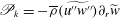 $\mathscr{P}_{k}=-\overline{{\it\rho}}(\widetilde{u^{\prime \prime }w^{\prime \prime }})\partial _{r}\widetilde{w}$
. Figures 8(a) and 8(b) shows
$\mathscr{P}_{k}=-\overline{{\it\rho}}(\widetilde{u^{\prime \prime }w^{\prime \prime }})\partial _{r}\widetilde{w}$
. Figures 8(a) and 8(b) shows
 $P_{k}$
near the inner and outer wall regions, respectively. From these results, it is clear that, while the mean strain rate
$P_{k}$
near the inner and outer wall regions, respectively. From these results, it is clear that, while the mean strain rate
 $\partial _{r}\widetilde{w}$
may increase due to the low dynamic viscosity near the hot inner wall (and decrease near the cold outer wall due to high dynamic viscosity), the decrease in the magnitude of the turbulent shear stress is in fact of higher importance to the production of turbulent kinetic energy.
$\partial _{r}\widetilde{w}$
may increase due to the low dynamic viscosity near the hot inner wall (and decrease near the cold outer wall due to high dynamic viscosity), the decrease in the magnitude of the turbulent shear stress is in fact of higher importance to the production of turbulent kinetic energy.

Figure 8. Production of turbulent kinetic energy in the reference case (I), forced
 $\text{sCO}_{2}$
convection case (II) and mixed
$\text{sCO}_{2}$
convection case (II) and mixed
 $\text{sCO}_{2}$
convection case (III).
$\text{sCO}_{2}$
convection case (III).
Table 4. Local Reynolds numbers for the simulated cases. In the last column
 ${\it\tau}$
denotes the turbulent shear stress
${\it\tau}$
denotes the turbulent shear stress
 $\overline{{\it\rho}}\widetilde{u^{\prime \prime }w^{\prime \prime }}$
.
$\overline{{\it\rho}}\widetilde{u^{\prime \prime }w^{\prime \prime }}$
.

3.3 Structures
While the previous section showed that the turbulent motions are affected by the mean dynamic viscosity and density stratification, it did not show whether the variable thermophysical property fluctuations can influence the turbulent motions of the fluid. It has been shown that near-wall turbulence may be regarded as a self-regenerating process, consisting of the formation of streamwise vortices and near-wall streaks as well as their instabilities (Waleffe Reference Waleffe1997; Jimenez & Pinelli Reference Jimenez and Pinelli1999; Schoppa & Hussain Reference Schoppa and Hussain2002). A flow may relaminarize if this self-regenerating process is disrupted (Jimenez & Pinelli Reference Jimenez and Pinelli1999; Kim Reference Kim2011). We will investigate here how near-wall streaks, which are largely responsible for
 $\overline{w^{\prime \prime }}^{2}$
, and streamwise vortices, which contribute to
$\overline{w^{\prime \prime }}^{2}$
, and streamwise vortices, which contribute to
 $\overline{u^{\prime \prime }}^{2}$
and
$\overline{u^{\prime \prime }}^{2}$
and
 $\overline{v^{\prime \prime }}^{2}$
, are affected by the fluctuations in thermophysical properties.
$\overline{v^{\prime \prime }}^{2}$
, are affected by the fluctuations in thermophysical properties.
In the simulations with variable density, the momentum
 ${\it\rho}\boldsymbol{u}$
is a conserved quantity. Furthermore, the density is continuous (as opposed to multiphase liquid flows, in which the density is discrete, for example). Therefore, to investigate structures that are relevant in the self-regenerating process, we chose to include the density in the mathematical description of a structure. To analyse streaks, we will look at
${\it\rho}\boldsymbol{u}$
is a conserved quantity. Furthermore, the density is continuous (as opposed to multiphase liquid flows, in which the density is discrete, for example). Therefore, to investigate structures that are relevant in the self-regenerating process, we chose to include the density in the mathematical description of a structure. To analyse streaks, we will look at
 $({\it\rho}w)^{\prime }<0$
, which for instance was also done by Duan, Beekman & Martin (Reference Duan, Beekman and Martin2011). Similarly, we will use the definition
$({\it\rho}w)^{\prime }<0$
, which for instance was also done by Duan, Beekman & Martin (Reference Duan, Beekman and Martin2011). Similarly, we will use the definition
 ${\it\chi}_{z}=(\boldsymbol{{\rm\nabla}}\times {\it\rho}\boldsymbol{u})_{z}=r^{-1}(\partial _{r}(r{\it\rho}v)-\partial _{{\it\theta}}({\it\rho}u))$
to analyse streamwise vortices. To distinguish from the classical vorticity
${\it\chi}_{z}=(\boldsymbol{{\rm\nabla}}\times {\it\rho}\boldsymbol{u})_{z}=r^{-1}(\partial _{r}(r{\it\rho}v)-\partial _{{\it\theta}}({\it\rho}u))$
to analyse streamwise vortices. To distinguish from the classical vorticity
 ${\bf\omega}=\boldsymbol{{\rm\nabla}}\times \boldsymbol{u}$
, we will call
${\bf\omega}=\boldsymbol{{\rm\nabla}}\times \boldsymbol{u}$
, we will call
 ${\bf\chi}\equiv \boldsymbol{{\rm\nabla}}\times {\it\rho}\boldsymbol{u}$
the momentum vorticity.
${\bf\chi}\equiv \boldsymbol{{\rm\nabla}}\times {\it\rho}\boldsymbol{u}$
the momentum vorticity.
An evolution equation can be derived for the momentum vorticity by taking the curl of (2.2). The complete derivation can be found in appendix C. The result can be written as
 $$\begin{eqnarray}\displaystyle \partial _{t}{\bf\chi} & = & \displaystyle -\boldsymbol{{\rm\nabla}}\times \boldsymbol{l}+Re^{-1}\boldsymbol{{\rm\nabla}}\boldsymbol{\cdot }{\it\mu}\boldsymbol{{\rm\nabla}}{\bf\omega}\nonumber\\ \displaystyle & & \displaystyle +\,Fr^{-1}\boldsymbol{{\rm\nabla}}\times {\it\rho}\hat{\boldsymbol{z}}-\boldsymbol{{\rm\nabla}}\times ({\it\psi}{\it\rho}\boldsymbol{u}+K\boldsymbol{{\rm\nabla}}{\it\rho})\nonumber\\ \displaystyle & & \displaystyle +\,Re^{-1}\boldsymbol{{\rm\nabla}}\boldsymbol{\cdot }(2\boldsymbol{{\rm\nabla}}{\it\mu}\times \unicode[STIX]{x1D64E}),\end{eqnarray}$$
in which
 $\boldsymbol{l}\equiv {\bf\chi}\times \boldsymbol{u}$
is the Lamb vector,
$\boldsymbol{l}\equiv {\bf\chi}\times \boldsymbol{u}$
is the Lamb vector,
 ${\it\psi}\equiv \boldsymbol{{\rm\nabla}}\boldsymbol{\cdot }\boldsymbol{u}$
the divergence of the velocity and
${\it\psi}\equiv \boldsymbol{{\rm\nabla}}\boldsymbol{\cdot }\boldsymbol{u}$
the divergence of the velocity and
 $K\equiv (\boldsymbol{u}\boldsymbol{\cdot }\boldsymbol{u})/2$
the kinetic energy. This equation clearly shows the contributions of the variable thermophysical properties, as the second line is equal to zero in constant-density flows, whereas the last term is equal to zero in constant-viscosity flows. For this reason, this equation will form the basis of our analysis of near-wall streak evolution and the generation of streamwise vortices. The physical interpretation of each term in (3.7) will be discussed for streaks and streamwise vortices separately, after an observational analysis is made first, in the following sections.
$K\equiv (\boldsymbol{u}\boldsymbol{\cdot }\boldsymbol{u})/2$
the kinetic energy. This equation clearly shows the contributions of the variable thermophysical properties, as the second line is equal to zero in constant-density flows, whereas the last term is equal to zero in constant-viscosity flows. For this reason, this equation will form the basis of our analysis of near-wall streak evolution and the generation of streamwise vortices. The physical interpretation of each term in (3.7) will be discussed for streaks and streamwise vortices separately, after an observational analysis is made first, in the following sections.
3.3.1 Generation of near-wall streaks
The variations in thermophysical properties in the
 $\text{sCO}_{2}$
cases (II and III) are found to have a clear effect on the streaks. Figure 9 shows the streaks near both the hot inner wall and the cold outer wall for the reference case (I) and the
$\text{sCO}_{2}$
cases (II and III) are found to have a clear effect on the streaks. Figure 9 shows the streaks near both the hot inner wall and the cold outer wall for the reference case (I) and the
 $\text{sCO}_{2}$
cases (II and III). The magnitude
$\text{sCO}_{2}$
cases (II and III). The magnitude
 $|({\it\rho}w)^{\prime }|$
of the streaks at the hot inner wall is reduced in the forced convection case (II, see figure 9
b) when compared to the reference case (I, see figure 9
a);
$|({\it\rho}w)^{\prime }|$
of the streaks at the hot inner wall is reduced in the forced convection case (II, see figure 9
b) when compared to the reference case (I, see figure 9
a);
 $|({\it\rho}w)^{\prime }|$
is further decreased in the mixed convection case (III, see figure 9
c). The reverse, however, is true for the cold wall:
$|({\it\rho}w)^{\prime }|$
is further decreased in the mixed convection case (III, see figure 9
c). The reverse, however, is true for the cold wall:
 $|({\it\rho}w)^{\prime }|$
is increased in the forced convection (II, see figure 9
e) and mixed convection (III, see figure 9
f) cases. The streaks also look slightly more disorganized in the forced convection case (II). This is even more so for the mixed convection case (III). As the ejections of streaks is largely responsible for the existence of the turbulent shear stress (Corino & Brodkey Reference Corino and Brodkey1969), the results described above are consistent with our earlier observations in § 3.2.2, where we observed that the magnitude of the turbulent shear stress decreases near the inner wall, and increases near the outer wall as a result of the variable thermophysical properties.
$|({\it\rho}w)^{\prime }|$
is increased in the forced convection (II, see figure 9
e) and mixed convection (III, see figure 9
f) cases. The streaks also look slightly more disorganized in the forced convection case (II). This is even more so for the mixed convection case (III). As the ejections of streaks is largely responsible for the existence of the turbulent shear stress (Corino & Brodkey Reference Corino and Brodkey1969), the results described above are consistent with our earlier observations in § 3.2.2, where we observed that the magnitude of the turbulent shear stress decreases near the inner wall, and increases near the outer wall as a result of the variable thermophysical properties.

Figure 9. Visualization of the streaks defined as
 $({\it\rho}w)^{\prime }<0$
near the hot (a–c) and cold (d–f) near-wall region (
$({\it\rho}w)^{\prime }<0$
near the hot (a–c) and cold (d–f) near-wall region (
 $y^{+}=5$
). Darker shades indicate larger values of
$y^{+}=5$
). Darker shades indicate larger values of
 $|({\it\rho}w)^{\prime }|$
. The direction of the flow is upwards. Only a part of the complete circumference is shown for the cold outer wall region.
$|({\it\rho}w)^{\prime }|$
. The direction of the flow is upwards. Only a part of the complete circumference is shown for the cold outer wall region.
To investigate the effect of variable thermophysical properties on the streaks in a quantitative manner, we will extract instantaneous density and dynamic viscosity data from individual streak realizations in a manner that is similar to the method described by Schoppa & Hussain (Reference Schoppa and Hussain2002):
-
(i) The location of local minima of
 $({\it\rho}w)^{\prime }$
, with respect to the circumferential direction, denoted as
${\it\theta}_{0}$
, are identified at constant
$y^{+}$
.
$({\it\rho}w)^{\prime }$
, with respect to the circumferential direction, denoted as
${\it\theta}_{0}$
, are identified at constant
$y^{+}$
. -
(ii) Data near the minima for different time instances are stored.
-
(iii) Data from the entire length of the streak and for different time instances are superimposed on each other, so that the minima of
$({\it\rho}w)^{\prime }$
are located at the same coordinate
$r^{-1}({\it\theta}-{\it\theta}_{0})$
. -
(iv) By averaging the data, average thermophysical properties of a streak are acquired.
-
(v) Any quantity
$(\cdots \,)$
that has been averaged according to the above described procedure will be denoted as
$\langle (\cdots \,)\rangle$
.


Figure 10(a,b) shows the result of the conditional averaging (streak extraction) procedure near the inner wall and the outer wall region, respectively, in the forced convection case (II). Just as streamwise vortices redistribute mean shear to create momentum streaks, they redistribute the mean density and dynamic viscosity profile, which in turn exist because of mean heat transfer from the hot inner wall to the cold outer wall. Therefore, streaks consist of low-density and low-dynamic-viscosity fluid, near the hot inner wall. This is consistent with observations by Cheng & Ng (Reference Cheng and Ng1982). The exact opposite is the case for the streaks near the cold outer wall (i.e. streaks have a high density and high dynamic viscosity). The thermophysical property gradients across the streaks are the physical interpretation of the thermophysical property fluctuations that were shown earlier in figure 4(c). The effect of these property gradients on the generation of streaks will subsequently be discussed.

Figure 10. Conditionally averaged profiles of the density and dynamic viscosity across a streak at
 $y^{+}=10$
. The dashed vertical lines represent the edges of the streak where
$y^{+}=10$
. The dashed vertical lines represent the edges of the streak where
 $r^{-1}\partial _{{\it\theta}}({\it\rho}w)^{\prime }=0$
.
$r^{-1}\partial _{{\it\theta}}({\it\rho}w)^{\prime }=0$
.
Jimenez & Pinelli (Reference Jimenez and Pinelli1999) investigated the evolution of streaks in a minimal box geometry by first deriving a parameter representative of streaks and subsequently deriving a transport equation for that parameter. Jimenez & Pinelli (Reference Jimenez and Pinelli1999) showed by artificially damping a source term in their streak evolution equation that turbulence can be suppressed or even completely quenched. In the current study, streaks depend mostly on the radial and circumferential coordinates
 $r$
and
$r$
and
 ${\it\theta}$
and they are coherent in the streamwise coordinate
${\it\theta}$
and they are coherent in the streamwise coordinate
 $z$
. In this study, however, streaks are not as well defined as they are in Jimenez & Pinelli (Reference Jimenez and Pinelli1999), because the annulus in this study is not a minimal box. We will therefore define the streak parameter as the conditional average
$z$
. In this study, however, streaks are not as well defined as they are in Jimenez & Pinelli (Reference Jimenez and Pinelli1999), because the annulus in this study is not a minimal box. We will therefore define the streak parameter as the conditional average
 $\langle \cdots \rangle$
of the radial component of the momentum vorticity
$\langle \cdots \rangle$
of the radial component of the momentum vorticity
 ${\bf\chi}$
:
${\bf\chi}$
:
 $$\begin{eqnarray}\langle {\it\chi}_{r}\rangle =\left\langle r^{-1}\partial _{{\it\theta}}({\it\rho}w)-\partial _{z}({\it\rho}v)\right\rangle =\left\langle r^{-1}\partial _{{\it\theta}}({\it\rho}w)^{\prime }-\partial _{z}({\it\rho}v)^{\prime }\right\rangle \approx \langle r^{-1}\partial _{{\it\theta}}({\it\rho}w)^{\prime }\rangle ,\end{eqnarray}$$
where we have used that
 $\partial _{{\it\theta}}(\overline{{\it\rho}w})=0$
. Therefore
$\partial _{{\it\theta}}(\overline{{\it\rho}w})=0$
. Therefore
 $\langle {\it\chi}_{r}\rangle$
may be thought of as the streamwise coherent streak flank strength and it is conceptually and physically close to the streak parameter that was defined by Jimenez & Pinelli (Reference Jimenez and Pinelli1999). After applying the conditional averaging operator
$\langle {\it\chi}_{r}\rangle$
may be thought of as the streamwise coherent streak flank strength and it is conceptually and physically close to the streak parameter that was defined by Jimenez & Pinelli (Reference Jimenez and Pinelli1999). After applying the conditional averaging operator
 $\langle \cdots \rangle$
to (3.7), an evolution equation for the streamwise coherent streak flank strength is obtained. The end result is written as:
$\langle \cdots \rangle$
to (3.7), an evolution equation for the streamwise coherent streak flank strength is obtained. The end result is written as:
 $$\begin{eqnarray}\displaystyle \partial _{t}\langle {\it\chi}_{r}\rangle & = & \displaystyle -\langle (\boldsymbol{{\rm\nabla}}\boldsymbol{\cdot }\boldsymbol{l})_{r}\rangle +Re^{-1}\langle \left(\boldsymbol{{\rm\nabla}}\boldsymbol{\cdot }{\it\mu}\boldsymbol{{\rm\nabla}}{\bf\omega}\right)_{r}\rangle \nonumber\\ \displaystyle & & \displaystyle +\,(r\,Fr)^{-1}\langle \partial _{{\it\theta}}{\it\rho}\rangle -\langle (\boldsymbol{{\rm\nabla}}\times K\boldsymbol{{\rm\nabla}}{\it\rho})_{r}\rangle -\langle (\boldsymbol{{\rm\nabla}}\times {\it\psi}{\it\rho}\boldsymbol{u})_{r}\rangle \nonumber\\ \displaystyle & & \displaystyle +\,Re^{-1}\langle \left(\boldsymbol{{\rm\nabla}}\boldsymbol{\cdot }2\boldsymbol{{\rm\nabla}}{\it\mu}\times \unicode[STIX]{x1D64E}\right)_{r}\rangle .\end{eqnarray}$$
We have assumed here that the operator
 $\langle \cdots \rangle$
is linear. It is clear that, for incompressible flows without variable thermophysical properties, all but the terms on the first line will be zero. Thus, the first line represents the evolution of streaks under constant thermophysical property conditions and it is the cylindrical counterpart to the streak evolution equation that is presented by Jimenez & Pinelli (Reference Jimenez and Pinelli1999). These first terms represent sources of the generation of streaks and diffusion of streaks, respectively. The terms on the second line all represent effects that may arise due to density gradients. The first term represents buoyancy, the second term involves a torque between kinetic energy and density gradients, while the third term is representative of thermal expansion effects, since, by (2.1),
$\langle \cdots \rangle$
is linear. It is clear that, for incompressible flows without variable thermophysical properties, all but the terms on the first line will be zero. Thus, the first line represents the evolution of streaks under constant thermophysical property conditions and it is the cylindrical counterpart to the streak evolution equation that is presented by Jimenez & Pinelli (Reference Jimenez and Pinelli1999). These first terms represent sources of the generation of streaks and diffusion of streaks, respectively. The terms on the second line all represent effects that may arise due to density gradients. The first term represents buoyancy, the second term involves a torque between kinetic energy and density gradients, while the third term is representative of thermal expansion effects, since, by (2.1),
 ${\it\psi}=\boldsymbol{{\rm\nabla}}\boldsymbol{\cdot }\boldsymbol{u}$
can be rewritten as
${\it\psi}=\boldsymbol{{\rm\nabla}}\boldsymbol{\cdot }\boldsymbol{u}$
can be rewritten as
 ${\it\psi}={\it\upsilon}^{-1}D_{t}{\it\upsilon}$
, where
${\it\psi}={\it\upsilon}^{-1}D_{t}{\it\upsilon}$
, where
 ${\it\upsilon}$
is the specific volume. The last term in the equation marks the effect of viscosity gradients on the evolution of streaks.
${\it\upsilon}$
is the specific volume. The last term in the equation marks the effect of viscosity gradients on the evolution of streaks.
This equation, however, may not be suited to quantify the effects of variable density and dynamic viscosity on the streak evolution with respect to the wall-normal distance, because all terms will vanish after circumferential averaging. Therefore, we multiply (3.9) with
 $\langle {\it\chi}_{r}\rangle$
and subsequently average it with respect to the circumferential direction over an interval that is equal to
$\langle {\it\chi}_{r}\rangle$
and subsequently average it with respect to the circumferential direction over an interval that is equal to
 $R_{in}{\rm\Delta}{\it\theta}^{+}=100$
and is centred on the streak centre. This interval is close to the spanwise length of the minimal box that was used by Jimenez & Pinelli (Reference Jimenez and Pinelli1999). The result is an evolution equation of what is in essence the magnitude of the streamwise coherent streak flank strength:
$R_{in}{\rm\Delta}{\it\theta}^{+}=100$
and is centred on the streak centre. This interval is close to the spanwise length of the minimal box that was used by Jimenez & Pinelli (Reference Jimenez and Pinelli1999). The result is an evolution equation of what is in essence the magnitude of the streamwise coherent streak flank strength:
 $$\begin{eqnarray}\displaystyle \partial _{t}\overline{\langle {\it\chi}_{r}\rangle ^{2}/2} & = & \displaystyle -\underbrace{\overline{\langle {\it\chi}_{r}\rangle \langle (\boldsymbol{{\rm\nabla}}\boldsymbol{\cdot }\boldsymbol{l})_{r}\rangle }}_{\text{sources}}+\underbrace{Re^{-1}\overline{\langle \left(\boldsymbol{{\rm\nabla}}\boldsymbol{\cdot }{\it\mu}\boldsymbol{{\rm\nabla}}{\bf\omega}\right)_{r}\rangle }}_{\text{diffusion and dissipation}}\nonumber\\ \displaystyle & & \displaystyle +\,\underbrace{Fr^{-1}\overline{\langle {\it\chi}_{r}\rangle r^{-1}\langle \partial _{{\it\theta}}{\it\rho}\rangle }}_{\text{buoyancy}}-\underbrace{\overline{\langle {\it\chi}_{r}\rangle \langle (\boldsymbol{{\rm\nabla}}\times K\boldsymbol{{\rm\nabla}}{\it\rho})_{r}\rangle }}_{\text{torque}}-\underbrace{\overline{\langle {\it\chi}_{r}\rangle \langle (\boldsymbol{{\rm\nabla}}\times {\it\psi}{\it\rho}\boldsymbol{u})_{r}\rangle }}_{\text{thermal expansion}}\nonumber\\ \displaystyle & & \displaystyle +\,\underbrace{Re^{-1}\overline{\langle {\it\chi}_{r}\rangle \langle \left(\boldsymbol{{\rm\nabla}}\boldsymbol{\cdot }2\boldsymbol{{\rm\nabla}}{\it\mu}\times \unicode[STIX]{x1D64E}\right)_{r}\rangle }}_{\text{viscosity gradient}},\end{eqnarray}$$
where
 $\overline{(\cdots \,)}$
represents an average with respect to the circumferential direction. We will use this equation not only to determine the magnitude of the variable properties effects on the evolution of streaks, but also to investigate where exactly such effects are important, with respect to the wall-normal distance. By multiplying (3.9) with
$\overline{(\cdots \,)}$
represents an average with respect to the circumferential direction. We will use this equation not only to determine the magnitude of the variable properties effects on the evolution of streaks, but also to investigate where exactly such effects are important, with respect to the wall-normal distance. By multiplying (3.9) with
 $\langle {\it\chi}_{r}\rangle$
, we have changed the meaning of the second term: it now represents the combined effects of diffusion and dissipation.
$\langle {\it\chi}_{r}\rangle$
, we have changed the meaning of the second term: it now represents the combined effects of diffusion and dissipation.

Figure 11. Budgets of the coherent streak flank strength
 $\mathscr{B}(\overline{\langle {\it\chi}_{r}\rangle ^{2}/2})$
, equation (3.10), in the reference case (I), the forced convection
$\mathscr{B}(\overline{\langle {\it\chi}_{r}\rangle ^{2}/2})$
, equation (3.10), in the reference case (I), the forced convection
 $\text{sCO}_{2}$
case (II) and the mixed convection
$\text{sCO}_{2}$
case (II) and the mixed convection
 $\text{sCO}_{2}$
case (III). The results have been scaled with bulk quantities.
$\text{sCO}_{2}$
case (III). The results have been scaled with bulk quantities.
The budgets of (3.10),
 $\mathscr{B}(\overline{\langle {\it\chi}_{r}\rangle ^{2}/2})$
, are shown for the reference case (I, in grey lines) and the forced convection and mixed convection
$\mathscr{B}(\overline{\langle {\it\chi}_{r}\rangle ^{2}/2})$
, are shown for the reference case (I, in grey lines) and the forced convection and mixed convection
 $\text{sCO}_{2}$
cases (II and III, in black lines) in figure 11. Near the inner wall (see figure 11
a), the magnitude of the regular sources in the
$\text{sCO}_{2}$
cases (II and III, in black lines) in figure 11. Near the inner wall (see figure 11
a), the magnitude of the regular sources in the
 $\text{sCO}_{2}$
cases is clearly smaller than that of the reference case (I). While the sources are balanced by only diffusion and dissipation in the reference case (I), it is clear that, in the
$\text{sCO}_{2}$
cases is clearly smaller than that of the reference case (I). While the sources are balanced by only diffusion and dissipation in the reference case (I), it is clear that, in the
 $\text{sCO}_{2}$
forced convection case (II), the sources are also balanced by thermal expansion, a kinetic energy gradient and density gradient torque and a viscosity gradient shear interaction near the inner wall. In the mixed convection case (III) (see figure 11
c), the sources are balanced by the effect of buoyancy as well. The kinetic energy gradient and density gradient torque has a modest, yet positive effect on the coherent flank strength near the inner wall. The thermal expansion has clearly a negative impact on the coherent streak flank strength, while the effect of viscosity gradient shear interaction has a very small, yet positive effect (near
$\text{sCO}_{2}$
forced convection case (II), the sources are also balanced by thermal expansion, a kinetic energy gradient and density gradient torque and a viscosity gradient shear interaction near the inner wall. In the mixed convection case (III) (see figure 11
c), the sources are balanced by the effect of buoyancy as well. The kinetic energy gradient and density gradient torque has a modest, yet positive effect on the coherent flank strength near the inner wall. The thermal expansion has clearly a negative impact on the coherent streak flank strength, while the effect of viscosity gradient shear interaction has a very small, yet positive effect (near
 $y^{+}=8$
) close to the inner wall. The influence of the thermal expansion has the largest influence.
$y^{+}=8$
) close to the inner wall. The influence of the thermal expansion has the largest influence.
Near the outer wall (see figure 11
b,d), the variable properties have a negligible effect, which is logical as the property variations are much smaller near the outer wall than near the inner wall. At the outer wall, the viscosity gradient shear interaction acts as a sink term close to the outer wall, and as a source term further away from it. The thermal expansion and buoyancy effects are positive. The kinetic energy and density gradient torque has the smallest contribution to the coherent streak flank strength near the outer wall or
 $y^{+}<10$
. The thermal expansion and buoyancy terms have opposite signs at the outer wall when compared with the inner wall. This can be explained as follows. The thermophysical property gradients across the streaks and high-speed fluid regions near the outer wall are of opposite sign when compared to the thermophysical property gradients across the streaks and high-speed fluid regions near the inner wall, as was shown in figure 10. From (3.10) it follows then that the variable thermophysical property effects on the coherent streak flank strength should be of opposite sign as well. These results for the budgets of the coherent streak flank strength indicate that the variable thermophysical properties have a significant effect on the formation of streaks. The most prominent variable thermophysical properties effects are thermal expansion and the kinetic energy gradient and density gradient torque.
$y^{+}<10$
. The thermal expansion and buoyancy terms have opposite signs at the outer wall when compared with the inner wall. This can be explained as follows. The thermophysical property gradients across the streaks and high-speed fluid regions near the outer wall are of opposite sign when compared to the thermophysical property gradients across the streaks and high-speed fluid regions near the inner wall, as was shown in figure 10. From (3.10) it follows then that the variable thermophysical property effects on the coherent streak flank strength should be of opposite sign as well. These results for the budgets of the coherent streak flank strength indicate that the variable thermophysical properties have a significant effect on the formation of streaks. The most prominent variable thermophysical properties effects are thermal expansion and the kinetic energy gradient and density gradient torque.
While (3.10) allowed us to quantify the effect of the variable thermophysical properties on the generation of streaks, it is interesting to investigate the meaning of (3.10) further. The effect of the buoyancy term in the mixed convection case (III) can be interpreted as follows. As streaks and high-speed fluid regions are formed by the streamwise advection of a streamwise vortex, they naturally have different densities, as was explained before (see also figure 10). Because a streak has a low density near the hot inner wall, the magnitude of the gravitational force that acts on it is smaller than the magnitude of the same force acting on a high-speed, high-density region. As a result, both the streaks, as well as the high-speed fluid regions, will be weakened. For example,
 $|({\it\rho}w)^{\prime }|$
will be smaller when compared to the forced convection case (II). At the cold outer wall, the opposite is true; the streaks have a high density, which results in a larger gravitational force on them, while the high-speed regions have a low density, which results in a smaller gravitational force acting on them. Therefore, the streaks and high-speed regions are enhanced near the cold outer wall (
$|({\it\rho}w)^{\prime }|$
will be smaller when compared to the forced convection case (II). At the cold outer wall, the opposite is true; the streaks have a high density, which results in a larger gravitational force on them, while the high-speed regions have a low density, which results in a smaller gravitational force acting on them. Therefore, the streaks and high-speed regions are enhanced near the cold outer wall (
 $|({\it\rho}w)^{\prime }|$
is enlarged by the gravitational force). The combination of density differences that exist across the streaks and the high-speed regions and the downward-pointing gravitational force acts in such a way that it counteracts the shear between the streak and high-speed region near the hot wall, while it enforces it near the cold wall. As streaks are weakened near the hot wall and enhanced near the cold wall, it can be said that the gravitational force has a stabilizing effect on the flow field near the hot wall and a destabilizing effect near the cold wall in the present configuration. This also became clear from examining the attenuated turbulent intensities in figure 7(c,d).
$|({\it\rho}w)^{\prime }|$
is enlarged by the gravitational force). The combination of density differences that exist across the streaks and the high-speed regions and the downward-pointing gravitational force acts in such a way that it counteracts the shear between the streak and high-speed region near the hot wall, while it enforces it near the cold wall. As streaks are weakened near the hot wall and enhanced near the cold wall, it can be said that the gravitational force has a stabilizing effect on the flow field near the hot wall and a destabilizing effect near the cold wall in the present configuration. This also became clear from examining the attenuated turbulent intensities in figure 7(c,d).
The term containing the divergence of the velocity (
 ${\it\psi}=\boldsymbol{{\rm\nabla}}\boldsymbol{\cdot }\boldsymbol{u}=r^{-1}\partial _{r}(ru)+r^{-1}\partial _{{\it\theta}}v+\partial _{z}w$
) in (3.10) suggests that the thermal expansion across the streaks and high-speed regions may be different. Figure 12 shows the divergence of the velocity at
${\it\psi}=\boldsymbol{{\rm\nabla}}\boldsymbol{\cdot }\boldsymbol{u}=r^{-1}\partial _{r}(ru)+r^{-1}\partial _{{\it\theta}}v+\partial _{z}w$
) in (3.10) suggests that the thermal expansion across the streaks and high-speed regions may be different. Figure 12 shows the divergence of the velocity at
 $y^{+}=5$
and
$y^{+}=5$
and
 $y^{+}=10$
with iso-lines of high-speed momentum superimposed. At
$y^{+}=10$
with iso-lines of high-speed momentum superimposed. At
 $y^{+}=5$
areas of positive thermal expansion coincide with high-speed momentum regions. However, this connection between thermal expansion and high-speed momentum does not seem to exist further away from the hot inner wall at
$y^{+}=5$
areas of positive thermal expansion coincide with high-speed momentum regions. However, this connection between thermal expansion and high-speed momentum does not seem to exist further away from the hot inner wall at
 $y^{+}=10$
. Instead, both negative and positive values of
$y^{+}=10$
. Instead, both negative and positive values of
 ${\it\psi}$
can be find across a high-speed region. This observation can be tested by calculating the expected value of
${\it\psi}$
can be find across a high-speed region. This observation can be tested by calculating the expected value of
 ${\it\psi}$
conditioned on the fluctuating streamwise momentum (variable conditioning was also used by Wang et al. (Reference Wang, Shi, Wang, Xiao, He and Chen2012)). The results for
${\it\psi}$
conditioned on the fluctuating streamwise momentum (variable conditioning was also used by Wang et al. (Reference Wang, Shi, Wang, Xiao, He and Chen2012)). The results for
 $y^{+}=5$
and
$y^{+}=5$
and
 $y^{+}=10$
are shown in figure 13. At
$y^{+}=10$
are shown in figure 13. At
 $y^{+}=5$
, the observation that areas of positive thermal expansion coincide with high-momentum fluid is indeed true. However, further away from the hot wall, this relation no longer exists. At
$y^{+}=5$
, the observation that areas of positive thermal expansion coincide with high-momentum fluid is indeed true. However, further away from the hot wall, this relation no longer exists. At
 $y^{+}=10$
, the instantaneous values of
$y^{+}=10$
, the instantaneous values of
 ${\it\psi}$
in figure 12 are large compared to the expected value of
${\it\psi}$
in figure 12 are large compared to the expected value of
 ${\it\psi}$
shown in figure 13. Therefore, areas of both positive and negative
${\it\psi}$
shown in figure 13. Therefore, areas of both positive and negative
 ${\it\psi}$
and can be found at a streak or a high-speed fluid region. The thermal expansion term in (3.10) can be interpreted as the effect that a high-speed fluid region or streak may consist of both positively and negatively expanding regions, which interfere with the coherence or the formation of streaks.
${\it\psi}$
and can be found at a streak or a high-speed fluid region. The thermal expansion term in (3.10) can be interpreted as the effect that a high-speed fluid region or streak may consist of both positively and negatively expanding regions, which interfere with the coherence or the formation of streaks.

Figure 12. Contour plots of
 $\boldsymbol{{\rm\nabla}}\boldsymbol{\cdot }\boldsymbol{u}$
in the
$\boldsymbol{{\rm\nabla}}\boldsymbol{\cdot }\boldsymbol{u}$
in the
 $({\it\theta},z)$
plane in the forced
$({\it\theta},z)$
plane in the forced
 $\text{sCO}_{2}$
case (II). The white lines indicate iso-lines of
$\text{sCO}_{2}$
case (II). The white lines indicate iso-lines of
 $({\it\rho}w)^{\prime }>0.2$
.
$({\it\rho}w)^{\prime }>0.2$
.

Figure 13. Expected value of
 $\boldsymbol{{\rm\nabla}}\boldsymbol{\cdot }\boldsymbol{u}$
conditioned on
$\boldsymbol{{\rm\nabla}}\boldsymbol{\cdot }\boldsymbol{u}$
conditioned on
 $({\it\rho}w)^{\prime }$
in the forced convection
$({\it\rho}w)^{\prime }$
in the forced convection
 $\text{sCO}_{2}$
case (II) at
$\text{sCO}_{2}$
case (II) at
 $y^{+}=5$
and
$y^{+}=5$
and
 $y^{+}=10$
.
$y^{+}=10$
.
The effect of the viscosity gradient shear interaction was earlier shown to act as a source term close to the hot inner wall. Thus
 $(\boldsymbol{{\rm\nabla}}\boldsymbol{\cdot }\langle \boldsymbol{{\rm\nabla}}{\it\mu}\times \unicode[STIX]{x1D64E}\rangle )_{r}$
can be expanded as (see Bladel Reference Bladel2007):
$(\boldsymbol{{\rm\nabla}}\boldsymbol{\cdot }\langle \boldsymbol{{\rm\nabla}}{\it\mu}\times \unicode[STIX]{x1D64E}\rangle )_{r}$
can be expanded as (see Bladel Reference Bladel2007):
 $$\begin{eqnarray}\displaystyle \overline{\langle {\it\chi}_{r}\rangle \langle \left(\boldsymbol{{\rm\nabla}}\boldsymbol{\cdot }\boldsymbol{{\rm\nabla}}{\it\mu}\times \unicode[STIX]{x1D64E}\right)_{r}\rangle } & = & \displaystyle \underbrace{\overline{\frac{\langle {\it\chi}_{r}\rangle }{r}\left\langle \frac{\partial }{\partial r}\left(rS_{zr}\frac{1}{r}\frac{\partial {\it\mu}}{\partial {\it\theta}}-rS_{{\it\theta}r}\frac{\partial {\it\mu}}{\partial z}\right)\right\rangle }}_{\text{A}}\nonumber\\ \displaystyle & & \displaystyle +\,\underbrace{\overline{\frac{\langle {\it\chi}_{r}\rangle }{r}\!\left\langle \frac{\partial }{\partial {\it\theta}}\!\left(S_{z{\it\theta}}\frac{1}{r}\frac{\partial {\it\mu}}{\partial {\it\theta}}-S_{{\it\theta}{\it\theta}}\frac{\partial {\it\mu}}{\partial z}\right)\!\right\rangle }}_{\text{B}}-\underbrace{\overline{\frac{\langle {\it\chi}_{r}\rangle }{r}\!\left\langle S_{r{\it\theta}}\frac{\partial {\it\mu}}{\partial z}-S_{z{\it\theta}}\frac{\partial {\it\mu}}{\partial r}\!\right\rangle }}_{\text{C}}\nonumber\\ \displaystyle & & \displaystyle +\,\underbrace{\overline{\frac{\langle {\it\chi}_{r}\rangle }{r}\left\langle \frac{\partial }{\partial z}\left(S_{{\it\theta}r}\frac{\partial {\it\mu}}{\partial r}-S_{rr}\frac{1}{r}\frac{\partial {\it\mu}}{\partial {\it\theta}}\right)\right\rangle }}_{\text{D}}.\end{eqnarray}$$
Closer investigation of these terms shows that the viscosity gradient shear interaction term is mostly determined by terms containing
 $r^{-1}\partial _{{\it\theta}}{\it\mu}$
and
$r^{-1}\partial _{{\it\theta}}{\it\mu}$
and
 $\partial _{z}{\it\mu}$
– more specifically, terms A and B in (3.11). This is shown in figure 14. In other words, the viscosity gradient shear interaction term is determined by dynamic viscosity fluctuations, instead of the mean radial dynamic viscosity profile.
$\partial _{z}{\it\mu}$
– more specifically, terms A and B in (3.11). This is shown in figure 14. In other words, the viscosity gradient shear interaction term is determined by dynamic viscosity fluctuations, instead of the mean radial dynamic viscosity profile.

Figure 14. Part of
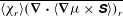 $\overline{\langle {\it\chi}_{r}\rangle (\boldsymbol{{\rm\nabla}}\boldsymbol{\cdot }\langle \boldsymbol{{\rm\nabla}}{\it\mu}\times \unicode[STIX]{x1D64E}\rangle )_{r}}$
that is determined by viscosity gradient fluctuations in the forced convection
$\overline{\langle {\it\chi}_{r}\rangle (\boldsymbol{{\rm\nabla}}\boldsymbol{\cdot }\langle \boldsymbol{{\rm\nabla}}{\it\mu}\times \unicode[STIX]{x1D64E}\rangle )_{r}}$
that is determined by viscosity gradient fluctuations in the forced convection
 $\text{sCO}_{2}$
case (II). Letters refer to (3.11).
$\text{sCO}_{2}$
case (II). Letters refer to (3.11).
3.3.2 Generation of streamwise vortical motions
Figure 15 shows instantaneous values of the streamwise momentum vorticity,
 ${\it\chi}_{z}$
, for the reference, forced convection
${\it\chi}_{z}$
, for the reference, forced convection
 $\text{sCO}_{2}$
(II) and mixed convection
$\text{sCO}_{2}$
(II) and mixed convection
 $\text{sCO}_{2}$
(III) cases. Streamwise momentum vorticity is clearly visible at both the inner wall and the outer wall in the reference case (I), while the streamwise momentum vorticity is much less apparent in the forced convection
$\text{sCO}_{2}$
(III) cases. Streamwise momentum vorticity is clearly visible at both the inner wall and the outer wall in the reference case (I), while the streamwise momentum vorticity is much less apparent in the forced convection
 $\text{sCO}_{2}$
case (II) near the inner wall. The streamwise momentum vorticity magnitude is not visibly decreased in the mixed convection case (III) near the inner wall. Both
$\text{sCO}_{2}$
case (II) near the inner wall. The streamwise momentum vorticity magnitude is not visibly decreased in the mixed convection case (III) near the inner wall. Both
 $\text{sCO}_{2}$
cases, however, show increased momentum vorticity near the outer wall, compared to the reference case (I). The decrease of streamwise momentum vorticity near the inner wall suggests diminished wall-normal and circumferential motion. Vice versa, an increase of momentum vorticity suggests enhanced wall-normal and circumferential motion. The observations of the streamwise momentum vorticity attenuation in the forced convection and mixed convection
$\text{sCO}_{2}$
cases, however, show increased momentum vorticity near the outer wall, compared to the reference case (I). The decrease of streamwise momentum vorticity near the inner wall suggests diminished wall-normal and circumferential motion. Vice versa, an increase of momentum vorticity suggests enhanced wall-normal and circumferential motion. The observations of the streamwise momentum vorticity attenuation in the forced convection and mixed convection
 $\text{sCO}_{2}$
cases (II and III) are therefore consistent with our observations of the turbulent intensities in figure 7. The r.m.s. values of streamwise momentum vorticity,
$\text{sCO}_{2}$
cases (II and III) are therefore consistent with our observations of the turbulent intensities in figure 7. The r.m.s. values of streamwise momentum vorticity,
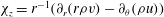 ${\it\chi}_{z}=r^{-1}(\partial _{r}(r{\it\rho}v)-\partial _{{\it\theta}}({\it\rho}u))$
, near the inner (figure 16
a) and outer wall (figure 16
b) reveal that the streamwise momentum vorticity has substantially decreased as a result of the property variations of the supercritical fluid near the inner wall and that it has increased near the outer wall. Near the inner wall, the difference between the inner wall in the forced convection
${\it\chi}_{z}=r^{-1}(\partial _{r}(r{\it\rho}v)-\partial _{{\it\theta}}({\it\rho}u))$
, near the inner (figure 16
a) and outer wall (figure 16
b) reveal that the streamwise momentum vorticity has substantially decreased as a result of the property variations of the supercritical fluid near the inner wall and that it has increased near the outer wall. Near the inner wall, the difference between the inner wall in the forced convection
 $\text{sCO}_{2}$
(II) and the mixed convection
$\text{sCO}_{2}$
(II) and the mixed convection
 $\text{sCO}_{2}$
(III) cases is negligible. Near the outer wall, however, the streamwise momentum vortices appear to be spatially slightly larger in the mixed convection
$\text{sCO}_{2}$
(III) cases is negligible. Near the outer wall, however, the streamwise momentum vortices appear to be spatially slightly larger in the mixed convection
 $\text{sCO}_{2}$
case (III) than they are in the forced convection
$\text{sCO}_{2}$
case (III) than they are in the forced convection
 $\text{sCO}_{2}$
case (II). The magnitude of the streamwise momentum vortices looks unaltered near the outer wall between the forced convection and mixed convection
$\text{sCO}_{2}$
case (II). The magnitude of the streamwise momentum vortices looks unaltered near the outer wall between the forced convection and mixed convection
 $\text{sCO}_{2}$
cases (II and III).
$\text{sCO}_{2}$
cases (II and III).

Figure 15. Cross-sectional visualization of the instantaneous streamwise momentum vorticity in the reference case (I), forced convection
 $\text{sCO}_{2}$
case (II) and mixed convection
$\text{sCO}_{2}$
case (II) and mixed convection
 $\text{sCO}_{2}$
case (III).
$\text{sCO}_{2}$
case (III).

Figure 16. R.m.s. values of the streamwise momentum vorticity in the near-wall regions in the reference case (I), forced convection
 $\text{sCO}_{2}$
case (II) and mixed convection
$\text{sCO}_{2}$
case (II) and mixed convection
 $\text{sCO}_{2}$
case (III).
$\text{sCO}_{2}$
case (III).
As before with the generation of streaks, we will use the evolution equation for momentum vorticity to investigate how variable thermophysical properties affect streamwise vortices. This equation is obtained by multiplying the streamwise component of (3.7) with
 ${\it\chi}_{z}$
. The result is written as
${\it\chi}_{z}$
. The result is written as
 $$\begin{eqnarray}\displaystyle \partial _{t}(\overline{{\it\chi}_{z}^{2}/2}) & = & \displaystyle -\underbrace{\overline{{\it\chi}_{z}(\boldsymbol{{\rm\nabla}}\times \boldsymbol{l})_{z}}}_{\text{sources}}+\underbrace{Re^{-1}\left(\overline{\boldsymbol{{\rm\nabla}}\boldsymbol{\cdot }{\it\chi}_{z}{\it\mu}\boldsymbol{{\rm\nabla}}{\it\omega}_{z}}\right)}_{\text{diffusion}}-\underbrace{Re^{-1}\overline{\boldsymbol{{\rm\nabla}}{\it\chi}_{z}\boldsymbol{\cdot }\boldsymbol{{\rm\nabla}}{\it\omega}_{z}}}_{\text{dissipation}}\nonumber\\ \displaystyle & & \displaystyle -\,\underbrace{\overline{{\it\chi}_{z}(\boldsymbol{{\rm\nabla}}\times {\it\psi}{\it\rho}\boldsymbol{u})_{z}}}_{\text{thermal expansion}}-\underbrace{\overline{{\it\chi}_{z}(\boldsymbol{{\rm\nabla}}K\times \boldsymbol{{\rm\nabla}}{\it\rho})_{z}}}_{\text{torque}}\nonumber\\ \displaystyle & & \displaystyle +\,\underbrace{Re^{-1}\overline{{\it\chi}_{z}\left(\boldsymbol{{\rm\nabla}}\boldsymbol{\cdot }2\boldsymbol{{\rm\nabla}}{\it\mu}\times \unicode[STIX]{x1D64E}\right)_{z}}}_{\text{viscosity gradient shear interaction}},\end{eqnarray}$$
where the first line represents sources, diffusion and dissipation of streamwise momentum vorticity, the second line represents the effects of variable density in the form of thermal expansion and a kinetic energy gradient and density gradient torque and where the third line represents the effect of variable dynamic viscosity shear interaction, as before. The buoyancy term is not shown here, because
 $Fr^{-1}(\boldsymbol{{\rm\nabla}}\times {\it\rho}\hat{\boldsymbol{z}})_{z}=\mathbf{0}$
, which suggests that the streamwise momentum vortices are not directly affected by buoyancy. This is also supported by the r.m.s. values of the streamwise momentum vorticity near the inner wall in figure 16.
$Fr^{-1}(\boldsymbol{{\rm\nabla}}\times {\it\rho}\hat{\boldsymbol{z}})_{z}=\mathbf{0}$
, which suggests that the streamwise momentum vortices are not directly affected by buoyancy. This is also supported by the r.m.s. values of the streamwise momentum vorticity near the inner wall in figure 16.

Figure 17. Budgets of the streamwise vorticity
 $\mathscr{B}(\overline{{\it\chi}_{z}^{2}/2})$
, equation (3.12). Black lines are used for the forced convection (II) and mixed convection (III)
$\mathscr{B}(\overline{{\it\chi}_{z}^{2}/2})$
, equation (3.12). Black lines are used for the forced convection (II) and mixed convection (III)
 $\text{sCO}_{2}$
cases, while grey lines are reserved for the reference case (I).
$\text{sCO}_{2}$
cases, while grey lines are reserved for the reference case (I).
The budgets
 $\mathscr{B}(\overline{{\it\chi}_{z}^{2}/2})$
of (3.12) are shown in figure 17 for the reference case (I) and the
$\mathscr{B}(\overline{{\it\chi}_{z}^{2}/2})$
of (3.12) are shown in figure 17 for the reference case (I) and the
 $\text{sCO}_{2}$
cases (II and III). Near the inner wall (figure 17
a,c), in both the forced convection and the mixed convection
$\text{sCO}_{2}$
cases (II and III). Near the inner wall (figure 17
a,c), in both the forced convection and the mixed convection
 $\text{sCO}_{2}$
cases (II and III), the contribution of the regular sources is smaller than it is in the reference case, except for a small region between
$\text{sCO}_{2}$
cases (II and III), the contribution of the regular sources is smaller than it is in the reference case, except for a small region between
 $y^{+}=8$
and
$y^{+}=8$
and
 $y^{+}=23$
for the forced convection case and between
$y^{+}=23$
for the forced convection case and between
 $y^{+}=10$
and
$y^{+}=10$
and
 $y^{+}=18$
for the mixed convection case. Near the outer wall, however (figure 17
b,d), the contribution of the regular sources is larger for all
$y^{+}=18$
for the mixed convection case. Near the outer wall, however (figure 17
b,d), the contribution of the regular sources is larger for all
 $y^{+}$
. The viscosity gradient shear interaction has a negligible effect on the formation of streamwise momentum vortices. The effect of thermal expansion is more significant than the variable viscosity effect, but only marginally. Both the variable viscosity and thermal expansion terms act as sink terms. The torque created by the kinetic energy and density gradients, however, has a significant effect, as it is larger than the combined effects of diffusion and dissipation near the inner wall in both the forced convection case (II) and the mixed convection case (III). This is not the case near the outer wall, where it is smaller, yet still substantial compared to regular sources. The torque acts as a sink near the inner wall, but as a source near the outer wall. The changes in the regular sources in the
$y^{+}$
. The viscosity gradient shear interaction has a negligible effect on the formation of streamwise momentum vortices. The effect of thermal expansion is more significant than the variable viscosity effect, but only marginally. Both the variable viscosity and thermal expansion terms act as sink terms. The torque created by the kinetic energy and density gradients, however, has a significant effect, as it is larger than the combined effects of diffusion and dissipation near the inner wall in both the forced convection case (II) and the mixed convection case (III). This is not the case near the outer wall, where it is smaller, yet still substantial compared to regular sources. The torque acts as a sink near the inner wall, but as a source near the outer wall. The changes in the regular sources in the
 $\text{sCO}_{2}$
cases (II and III) compared to the reference case (I) combined with the effects of the torque explains why the r.m.s. values of the streamwise momentum vortices of figure 16 are smaller in the
$\text{sCO}_{2}$
cases (II and III) compared to the reference case (I) combined with the effects of the torque explains why the r.m.s. values of the streamwise momentum vortices of figure 16 are smaller in the
 $\text{sCO}_{2}$
cases (II and III) near the inner wall and larger near the outer wall. The fact that the regular sources are larger near the outer wall in the mixed convection case (III) than in the forced convection case (II) is consistent with the r.m.s. values near the outer wall as well.
$\text{sCO}_{2}$
cases (II and III) near the inner wall and larger near the outer wall. The fact that the regular sources are larger near the outer wall in the mixed convection case (III) than in the forced convection case (II) is consistent with the r.m.s. values near the outer wall as well.

Figure 18. Four depictions of the same burst of a low-speed, low-density region near the inner wall in the wall-normal plane. (a) The momentum vector field (not all vectors are shown). The solid contour lines indicate positive streamwise vorticity, while the dashed contour lines indicate negative streamwise momentum vorticity. (b) The iso-density lines (black) and the iso-kinetic energy lines (white). (c) The gradient vectors (not to scale) of the kinetic energy (white) and the density (black). (d) The locations of positive and negative streamwise vorticity that are induced by the kinetic energy gradient and density gradient torque.
The torque effect can be further clarified by looking at figure 18. In this figure, a typical ejection of low-speed, low-density fluid near the hot inner wall is shown. This ejection generates a region of negative streamwise momentum vorticity
 ${\it\chi}_{z}^{-}$
and a region of positive streamwise momentum vorticity
${\it\chi}_{z}^{-}$
and a region of positive streamwise momentum vorticity
 ${\it\chi}_{z}^{+}$
, which have been marked by black iso-lines superimposed on the vector field
${\it\chi}_{z}^{+}$
, which have been marked by black iso-lines superimposed on the vector field
 $({\it\rho}u,{\it\rho}v)^{\text{T}}$
in figure 18(a). The iso-contours of the kinetic energy and the density, shown in figure 18(b), are clearly not parallel, which indicates that
$({\it\rho}u,{\it\rho}v)^{\text{T}}$
in figure 18(a). The iso-contours of the kinetic energy and the density, shown in figure 18(b), are clearly not parallel, which indicates that
 $-\boldsymbol{{\rm\nabla}}K\times \boldsymbol{{\rm\nabla}}{\it\rho}=\boldsymbol{{\rm\nabla}}{\it\rho}\times \boldsymbol{{\rm\nabla}}K$
is non-zero. Figure 18(c) shows the kinetic energy and density gradient vectors. In the inner part of the mushroom-like structure (region A and
$-\boldsymbol{{\rm\nabla}}K\times \boldsymbol{{\rm\nabla}}{\it\rho}=\boldsymbol{{\rm\nabla}}{\it\rho}\times \boldsymbol{{\rm\nabla}}K$
is non-zero. Figure 18(c) shows the kinetic energy and density gradient vectors. In the inner part of the mushroom-like structure (region A and
 $\text{A}^{\prime }$
), the torque acts to create a region of positive streamwise momentum vorticity near A and a region of negative streamwise momentum vorticity near
$\text{A}^{\prime }$
), the torque acts to create a region of positive streamwise momentum vorticity near A and a region of negative streamwise momentum vorticity near
 $\text{A}^{\prime }$
(see figure 18
d). At the top of the mushroom-like structure (region B and
$\text{A}^{\prime }$
(see figure 18
d). At the top of the mushroom-like structure (region B and
 $\text{B}^{\prime }$
), the opposite occurs: the torque acts to create negative streamwise vorticity near
$\text{B}^{\prime }$
), the opposite occurs: the torque acts to create negative streamwise vorticity near
 $\text{B}^{\prime }$
and positive streamwise vorticity near B. Therefore, the torque between the kinetic energy gradient and the density gradient both counteracts as well as aids the streamwise momentum vorticity generated by the unstable low-speed region. It is clear that the kinetic energy and density gradient vectors are almost parallel at the top, yet almost perpendicular to each other inside the mushroom-like structure. Thus, the magnitude of the torque is much smaller at the top near B and
$\text{B}^{\prime }$
and positive streamwise vorticity near B. Therefore, the torque between the kinetic energy gradient and the density gradient both counteracts as well as aids the streamwise momentum vorticity generated by the unstable low-speed region. It is clear that the kinetic energy and density gradient vectors are almost parallel at the top, yet almost perpendicular to each other inside the mushroom-like structure. Thus, the magnitude of the torque is much smaller at the top near B and
 $\text{B}^{\prime }$
(as parallel gradients of the kinetic energy and density result in
$\text{B}^{\prime }$
(as parallel gradients of the kinetic energy and density result in
 $\boldsymbol{{\rm\nabla}}{\it\rho}\times \boldsymbol{{\rm\nabla}}K=\mathbf{0}$
) than the magnitude of the torque near the inner part near A and
$\boldsymbol{{\rm\nabla}}{\it\rho}\times \boldsymbol{{\rm\nabla}}K=\mathbf{0}$
) than the magnitude of the torque near the inner part near A and
 $\text{A}^{\prime }$
(where
$\text{A}^{\prime }$
(where
 $\boldsymbol{{\rm\nabla}}{\it\rho}$
and
$\boldsymbol{{\rm\nabla}}{\it\rho}$
and
 $\boldsymbol{{\rm\nabla}}K$
make an almost
$\boldsymbol{{\rm\nabla}}K$
make an almost
 $90^{\circ }$
angle). The net result is that the torque acts as a sink term to the formation of streamwise momentum vorticity near a hot inner wall, which was also shown in figure 17. At the cold outer wall, high-density fluid is ejected instead of low-density fluid. This means that, for a similar mushroom-like structure near the outer wall, the density gradient vector is of opposite sign when compared to the same vector near the inner wall. Therefore, near the outer wall, the kinetic energy gradient and density gradient torque acts as a source term for the formation of streamwise momentum vorticity on average, which can also be seen in figure 17. From the direction of the density gradient vector near the inner part of the mushroom-like structure it is clear that both
$90^{\circ }$
angle). The net result is that the torque acts as a sink term to the formation of streamwise momentum vorticity near a hot inner wall, which was also shown in figure 17. At the cold outer wall, high-density fluid is ejected instead of low-density fluid. This means that, for a similar mushroom-like structure near the outer wall, the density gradient vector is of opposite sign when compared to the same vector near the inner wall. Therefore, near the outer wall, the kinetic energy gradient and density gradient torque acts as a source term for the formation of streamwise momentum vorticity on average, which can also be seen in figure 17. From the direction of the density gradient vector near the inner part of the mushroom-like structure it is clear that both
 $\partial _{r}{\it\rho}$
as well as
$\partial _{r}{\it\rho}$
as well as
 $r^{-1}\partial _{{\it\theta}}{\it\rho}$
are important here, which shows that the density fluctuations are important to the generation of streamwise vortices and thus in the turbulence attenuation that may occur in heated or cooled turbulent flows at supercritical pressure.
$r^{-1}\partial _{{\it\theta}}{\it\rho}$
are important here, which shows that the density fluctuations are important to the generation of streamwise vortices and thus in the turbulence attenuation that may occur in heated or cooled turbulent flows at supercritical pressure.
3.4 Molecular Prandtl-number effect
In the previous discussion, it has become clear that thermophysical property fluctuations that occur as a result of the self-regenerating process play an important role in the generation of streaks and streamwise momentum vorticity. In this section, we will investigate how variable property effects scale between the forced convection
 $\text{sCO}_{2}$
case (II), the variable density case (IV) and the variable dynamic viscosity case (V). The magnitude of the thermophysical property fluctuations is only determined by the magnitude of the enthalpy fluctuations (under the low-Mach-number approximation assumption), which are in turn determined by the Reynolds number and the molecular Prandtl number. The variable thermophysical property effects on the generation of streaks and streamwise momentum vorticity should then be determined by the Prandtl number as well. In turbulent flows, gradients of fluctuations are typically larger then gradients of mean quantities (see e.g. Tennekes & Lumley Reference Tennekes and Lumley1972). Following Tennekes & Lumley (Reference Tennekes and Lumley1972), we will choose
$\text{sCO}_{2}$
case (II), the variable density case (IV) and the variable dynamic viscosity case (V). The magnitude of the thermophysical property fluctuations is only determined by the magnitude of the enthalpy fluctuations (under the low-Mach-number approximation assumption), which are in turn determined by the Reynolds number and the molecular Prandtl number. The variable thermophysical property effects on the generation of streaks and streamwise momentum vorticity should then be determined by the Prandtl number as well. In turbulent flows, gradients of fluctuations are typically larger then gradients of mean quantities (see e.g. Tennekes & Lumley Reference Tennekes and Lumley1972). Following Tennekes & Lumley (Reference Tennekes and Lumley1972), we will choose
 $\mathscr{U}$
to be a reference velocity scale and
$\mathscr{U}$
to be a reference velocity scale and
 ${\it\lambda}$
to be the Taylor micro-scale. The gradient of a velocity fluctuation then is
${\it\lambda}$
to be the Taylor micro-scale. The gradient of a velocity fluctuation then is
 $\mathit{O}(\mathscr{U}/{\it\lambda})$
. Then, if
$\mathit{O}(\mathscr{U}/{\it\lambda})$
. Then, if
 ${\it\lambda}_{th}$
is the thermal energy analogue of
${\it\lambda}_{th}$
is the thermal energy analogue of
 ${\it\lambda}$
and
${\it\lambda}$
and
 $\mathscr{R}$
the reference density scale, it follows for density gradient fluctuations that
$\mathscr{R}$
the reference density scale, it follows for density gradient fluctuations that
 $$\begin{eqnarray}\boldsymbol{{\rm\nabla}}{\it\rho}\propto \mathit{O}\,\left(\frac{\mathscr{R}}{{\it\lambda}_{th}}\right)=\mathit{O}\left(\frac{\mathscr{R}}{{\it\lambda}}\frac{{\it\lambda}}{{\it\lambda}_{th}}\right)=\mathit{O}\left(\frac{\mathscr{R}}{{\it\lambda}}\sqrt{Pr}\right).\end{eqnarray}$$
We used here that
 ${\it\lambda}/{\it\lambda}_{th}=\sqrt{Pr}$
(see Batchelor Reference Batchelor1959). Similar arguments can be made for the divergence of the velocity:
${\it\lambda}/{\it\lambda}_{th}=\sqrt{Pr}$
(see Batchelor Reference Batchelor1959). Similar arguments can be made for the divergence of the velocity:
 $$\begin{eqnarray}\boldsymbol{{\rm\nabla}}\boldsymbol{\cdot }\boldsymbol{u}\propto \mathit{O}\left(\frac{\mathscr{U}}{{\it\lambda}_{th}}\right)=\mathit{O}\left(\frac{\mathscr{U}}{{\it\lambda}}\frac{{\it\lambda}}{{\it\lambda}_{th}}\right)=\mathit{O}\left(\frac{\mathscr{U}}{{\it\lambda}}\sqrt{Pr}\right).\end{eqnarray}$$
A similar estimate can be made for viscosity gradient fluctuations, but since the variable density effects are of greater importance to the generation of streaks and streamwise momentum vorticity, we will focus on the variable density effects only. The scaling estimates (3.13) and (3.14) suggest that, if
 $\mathscr{R}$
(or
$\mathscr{R}$
(or
 $\mathscr{U}$
) and
$\mathscr{U}$
) and
 ${\it\lambda}$
are kept constant under different conditions, then any property gradient term in (3.10) and (3.12) should scale with
${\it\lambda}$
are kept constant under different conditions, then any property gradient term in (3.10) and (3.12) should scale with
 $\sqrt{Pr}$
. Qualitatively, this suggests that the magnitude of the variable property effects between the
$\sqrt{Pr}$
. Qualitatively, this suggests that the magnitude of the variable property effects between the
 $\text{sCO}_{2}$
forced convection case (II) and the variable density (IV) or dynamic viscosity case (V) scale with a factor of
$\text{sCO}_{2}$
forced convection case (II) and the variable density (IV) or dynamic viscosity case (V) scale with a factor of
 ${\it\gamma}\equiv (\overline{Pr}^{\,forced}/Pr^{ref})^{1/2}$
, if
${\it\gamma}\equiv (\overline{Pr}^{\,forced}/Pr^{ref})^{1/2}$
, if
 ${\it\lambda}$
remains the same (which is reasonable because the local Reynolds numbers are very similar). Note that
${\it\lambda}$
remains the same (which is reasonable because the local Reynolds numbers are very similar). Note that
 $\overline{Pr}^{\,forced}$
refers to the average molecular Prandtl number in case II (which varies from 1.6 to 12), while
$\overline{Pr}^{\,forced}$
refers to the average molecular Prandtl number in case II (which varies from 1.6 to 12), while
 $Pr^{ref}$
refers to the molecular Prandtl number in cases I, IV and V (which is equal to 2.85). Figure 19 shows the factor
$Pr^{ref}$
refers to the molecular Prandtl number in cases I, IV and V (which is equal to 2.85). Figure 19 shows the factor
 ${\it\gamma}$
as a function of the wall distance. The profile of
${\it\gamma}$
as a function of the wall distance. The profile of
 ${\it\gamma}$
suggests that the variable property effects of the
${\it\gamma}$
suggests that the variable property effects of the
 $\text{sCO}_{2}$
case (II) should be smaller than those of the variable density and dynamic viscosity cases for
$\text{sCO}_{2}$
case (II) should be smaller than those of the variable density and dynamic viscosity cases for
 $y^{+}<5$
and vice versa for
$y^{+}<5$
and vice versa for
 $y^{+}>5$
.
$y^{+}>5$
.

Figure 19. The factor
 ${\it\gamma}\equiv (\overline{Pr}^{\,forced}/Pr^{ref})^{1/2}$
as a function of the inner wall distance. The vertical dotted line denotes the position where
${\it\gamma}\equiv (\overline{Pr}^{\,forced}/Pr^{ref})^{1/2}$
as a function of the inner wall distance. The vertical dotted line denotes the position where
 $\overline{Pr}^{\,forced}=Pr^{ref}$
.
$\overline{Pr}^{\,forced}=Pr^{ref}$
.

Figure 20. Comparison of the thermal expansion term (a) and kinetic energy gradient and density gradient torque (b) in (3.10) between the
 $\text{sCO}_{2}$
forced convection case (II) and the constant molecular
$\text{sCO}_{2}$
forced convection case (II) and the constant molecular
 $Pr$
cases (grey lines). The vertical dotted line denotes the position where
$Pr$
cases (grey lines). The vertical dotted line denotes the position where
 $\overline{Pr}^{\,forced}=Pr^{ref}$
.
$\overline{Pr}^{\,forced}=Pr^{ref}$
.

Figure 21. Comparison of the kinetic energy gradient and density gradient torque equation (3.12) between the
 $\text{sCO}_{2}$
forced convection case (black lines) and the variable density case (grey lines). The vertical dotted line denotes the position where
$\text{sCO}_{2}$
forced convection case (black lines) and the variable density case (grey lines). The vertical dotted line denotes the position where
 $\overline{Pr}^{\,forced}=Pr^{ref}$
.
$\overline{Pr}^{\,forced}=Pr^{ref}$
.
Figure 20 shows again the thermal expansion term and the kinetic energy gradient and density gradient torque of (3.10), but now for both the
 $\text{sCO}_{2}$
case (II) and the variable density (IV) case. The region where the thermal expansion effect in the variable density case (IV) is larger than that of the
$\text{sCO}_{2}$
case (II) and the variable density (IV) case. The region where the thermal expansion effect in the variable density case (IV) is larger than that of the
 $\text{sCO}_{2}$
forced convection
$\text{sCO}_{2}$
forced convection
 $\text{sCO}_{2}$
case (II) is found for
$\text{sCO}_{2}$
case (II) is found for
 $y^{+}<6$
, which is close to the point where
$y^{+}<6$
, which is close to the point where
 $\overline{Pr}^{\,forced}=Pr^{\,ref}$
. It can be seen that the thermal expansion effect in the forced convection
$\overline{Pr}^{\,forced}=Pr^{\,ref}$
. It can be seen that the thermal expansion effect in the forced convection
 $\text{sCO}_{2}$
case shows a sudden increase near
$\text{sCO}_{2}$
case shows a sudden increase near
 $y^{+}=10$
, when compared with the variable density case (IV). This is logical according to estimate (3.14), as
$y^{+}=10$
, when compared with the variable density case (IV). This is logical according to estimate (3.14), as
 ${\it\gamma}$
strongly increases around
${\it\gamma}$
strongly increases around
 $y^{+}=10$
(see figure 19), with respect to the wall-normal distance. The physical interpretation is that, due to the increase of the Prandtl number with
$y^{+}=10$
(see figure 19), with respect to the wall-normal distance. The physical interpretation is that, due to the increase of the Prandtl number with
 $y^{+}$
, the thermal fluctuations will increase with
$y^{+}$
, the thermal fluctuations will increase with
 $y^{+}$
in the forced convection
$y^{+}$
in the forced convection
 $\text{sCO}_{2}$
case when compared to the variable density case (IV), which results in the sudden increase in the magnitude of the thermal expansion term.
$\text{sCO}_{2}$
case when compared to the variable density case (IV), which results in the sudden increase in the magnitude of the thermal expansion term.
The kinetic energy gradient and density gradient torque shows a similar trend as the thermal expansion term. The torque is smaller in the forced convection
 $\text{sCO}_{2}$
case (II) for
$\text{sCO}_{2}$
case (II) for
 $y^{+}<4.3$
than it is in the variable density case (IV). For
$y^{+}<4.3$
than it is in the variable density case (IV). For
 $y^{+}>5$
, the torque effect is much larger in the
$y^{+}>5$
, the torque effect is much larger in the
 $\text{sCO}_{2}$
case (II). Near
$\text{sCO}_{2}$
case (II). Near
 $y^{+}=10$
, the torque is slightly negative in the variable density case (IV), while in the forced convection
$y^{+}=10$
, the torque is slightly negative in the variable density case (IV), while in the forced convection
 $\text{sCO}_{2}$
case it is slightly positive: this difference cannot be explained by the scaling estimate (3.13).
$\text{sCO}_{2}$
case it is slightly positive: this difference cannot be explained by the scaling estimate (3.13).
The effect of the kinetic energy gradient and density gradient torque on streamwise vorticity is shown in figure 21. The region where the kinetic energy gradient and density gradient torque is larger in the variable density case (IV) than it is in the forced convection
 $\text{sCO}_{2}$
(II) case is found for
$\text{sCO}_{2}$
(II) case is found for
 $y^{+}<8.6$
. Before, we assumed that
$y^{+}<8.6$
. Before, we assumed that
 ${\it\lambda}$
would be constant between the cases. However, if we assume that this does not hold for the momentum vorticity length scales, the scaling estimate (3.13) suggests that the effect of the kinetic energy gradient and density gradient torque in the forced convection
${\it\lambda}$
would be constant between the cases. However, if we assume that this does not hold for the momentum vorticity length scales, the scaling estimate (3.13) suggests that the effect of the kinetic energy gradient and density gradient torque in the forced convection
 $\text{sCO}_{2}$
case (II) to that of the variable density case (IV) scales as
$\text{sCO}_{2}$
case (II) to that of the variable density case (IV) scales as
 $({\it\lambda}^{IV}/{\it\lambda}^{II}){\it\gamma}$
. This suggests that the spatial scales of the streamwise momentum vorticity are different between the
$({\it\lambda}^{IV}/{\it\lambda}^{II}){\it\gamma}$
. This suggests that the spatial scales of the streamwise momentum vorticity are different between the
 $\text{sCO}_{2}$
(II and III) and variable density (IV) cases.
$\text{sCO}_{2}$
(II and III) and variable density (IV) cases.
While the scaling arguments that were made above should be seen as a qualitative analysis, it is reasonable to assume that the variable Prandtl number of fluids at supercritical pressure has a clear effect on the evolution of turbulent structures, through the magnitude of the variation of the density gradients.
4 Conclusions
In this paper, we have investigated by means of DNS the effect of variable thermophysical properties of supercritical fluids on a turbulent annular flow that is heated at the inner wall and cooled at the outer wall. Near the inner wall, the fluid has a low density and dynamic viscosity and vice versa at the outer wall. Owing to the fact that the two walls are kept at different temperatures, a mean radial dynamic viscosity and density profile exists. Large density and viscosity variations were found near the inner wall.
While looking at classical turbulent statistics, it was found that the mean velocity profiles, turbulent shear stresses and turbulent intensities were significantly affected by the mean variation in dynamic viscosity and density. The differences in mean strain rate and turbulent shear stresses lead to a decreased production of turbulent kinetic energy near the hot inner wall and an enhanced production near the outer wall. However, these observations did not show if the variable properties have a direct influence on turbulent motions. To investigate further, turbulent structures were analysed in detail.
As streamwise momentum vortices interact with the mean velocity to create streaks, they also interact with the mean density and mean dynamic viscosity. As a result, low-speed streaks near the hot wall have a low density and dynamic viscosity, compared to the high-speed fluid that surrounds them. Both positive and negative thermal expansion regions existing within the streaks were found to have a negative impact on the coherence of the streaks. The dynamic viscosity gradient across the streaks was observed to act as a source term very close to the inner wall and to be negligible when compared to variable density effects. Buoyancy acts to counteract the shear between low-density momentum streaks and high-density, high-speed regions in buoyancy-opposed flow. The opposite holds for the cold outer wall, as the thermophysical property gradients across the streaks are of opposite sign compared to the gradients across the streaks near the inner wall. The density and dynamic viscosity fluctuations therefore influence the streamwise momentum fluctuations directly.
The streamwise vorticity was found to be negligibly affected by the dynamic viscosity fluctuations and thermal expansion. However, the torque between the kinetic energy gradient and the density gradient was found to act as a very large sink term near the inner wall and as a source term near the outer wall. It was shown that streamwise momentum vorticity, created by the instability of a low-speed region, is counteracted or enhanced by this torque. Both the radial density gradient as well as the circumferential density gradient were found to be important; the density and dynamic viscosity fluctuations therefore also influence the wall-normal and circumferential turbulent motions of the fluid.
As both streaks and streamwise vortices are important to the self-regenerating near-wall cycle, it is feasible that a complete disruption of this cycle, and thus relaminarization, may occur as a result of thermal expansion, a viscosity gradient shear interaction, buoyancy as well as a kinetic energy gradient and density gradient torque in heated supercritical fluids. In other words, local thermophysical property variations can be responsible for decreased or increased turbulent motions in heated or cooled fluids at supercritical pressure.
Acknowledgement
This research is supported by the Dutch Technology Foundation STW, which is part of the Netherlands Organisation for Scientific Research (NWO), and which is partly funded by the Ministry of Economic Affairs. We would hereby like to acknowledge that the results of this research were achieved while using the PRACE research infrastructure resources Cartesius (based in the Netherlands at SURFsara) and Anselm (based in the Czech Republic at IT4Innovations).

Figure 22. (a) Wall-normal mesh width and (b) radial distance versus grid point number according to (A 1) for
 $N=256$
.
$N=256$
.

Figure 23. (a) Streamwise and (b) circumferential power spectra of enthalpy fluctuations. Curve A corresponds to the location where
 $h_{rms}$
is largest, and curve B refers to the location where
$h_{rms}$
is largest, and curve B refers to the location where
 $\overline{Pr}$
is largest.
$\overline{Pr}$
is largest.
Appendix A. Mesh generation and enthalpy power spectra
The wall-normal mesh size is calculated according to
 $$\begin{eqnarray}{\rm\Delta}r(n)=\frac{1}{0.65}\left(\frac{1/8}{N}+6\frac{n^{4}}{N^{5}}-12\frac{n^{3}}{N^{4}}+6\frac{n^{2}}{N^{3}}\right),\end{eqnarray}$$
where
 ${\rm\Delta}r$
is the wall-normal size,
${\rm\Delta}r$
is the wall-normal size,
 $n$
the grid number and
$n$
the grid number and
 $N$
the total number of grid points in the wall-normal direction. This leads to a modest stretching of the cells, as can be seen in figure 22(a,b). Power spectra of the enthalpy fluctuations are shown in figure 23(a,b) for the streamwise and circumferential directions, respectively, at two different points (A and B) in the forced convection
$N$
the total number of grid points in the wall-normal direction. This leads to a modest stretching of the cells, as can be seen in figure 22(a,b). Power spectra of the enthalpy fluctuations are shown in figure 23(a,b) for the streamwise and circumferential directions, respectively, at two different points (A and B) in the forced convection
 $\text{sCO}_{2}$
case. Point A refers to the wall-normal location where the enthalpy fluctuations are the largest (near the hot wall), while point B corresponds to the wall-normal location where the mean molecular Prandtl number has its maximum. At point A at least six decades are resolved, while at point B at least three decades are resolved. There is a small build-up of energy at the highest wavenumbers, which is assumed to be too small to affect the results in this paper. As the momentum scales are larger than the thermal scales for Prandtl numbers larger than unity, the mesh can be considered to be sufficient to resolve all momentum scales.
$\text{sCO}_{2}$
case. Point A refers to the wall-normal location where the enthalpy fluctuations are the largest (near the hot wall), while point B corresponds to the wall-normal location where the mean molecular Prandtl number has its maximum. At point A at least six decades are resolved, while at point B at least three decades are resolved. There is a small build-up of energy at the highest wavenumbers, which is assumed to be too small to affect the results in this paper. As the momentum scales are larger than the thermal scales for Prandtl numbers larger than unity, the mesh can be considered to be sufficient to resolve all momentum scales.
Appendix B. Validation of buoyancy influence
Because the effect of buoyancy is also studied in the present study, the code was also validated against two experiments by Carr, Connor & Buhr (Reference Carr, Connor and Buhr1973). In these experiments, denoted as
 $N_{10}$
and
$N_{10}$
and
 $N_{12}$
, upward-flowing air (at a bulk Reynolds number of 5300) is heated in a pipe at atmospheric pressure. The same system was simulated using the code on a mesh with
$N_{12}$
, upward-flowing air (at a bulk Reynolds number of 5300) is heated in a pipe at atmospheric pressure. The same system was simulated using the code on a mesh with
 $128\times 256\times 256$
grid points and a domain length of six hydraulic diameters. Mean velocity and temperature measurements are compared with the results from the DNS in figure 24(a) and the turbulent heat flux is compared in figure 24(b). The results validate the code, since there is good agreement between the DNS results and the measured experimental data.
$128\times 256\times 256$
grid points and a domain length of six hydraulic diameters. Mean velocity and temperature measurements are compared with the results from the DNS in figure 24(a) and the turbulent heat flux is compared in figure 24(b). The results validate the code, since there is good agreement between the DNS results and the measured experimental data.

Figure 24. Comparison between the current DNS code and the experiment described by Carr et al. (Reference Carr, Connor and Buhr1973). The symbols denote experimental values, while the lines represent results of direct numerical simulations:
 $N_{10}$
, solid symbols and continuous lines;
$N_{10}$
, solid symbols and continuous lines;
 $N_{12}$
, open symbols and dashed lines.
$N_{12}$
, open symbols and dashed lines.
Appendix C. Derivation of the momentum vorticity evolution equation
Here, we will show how the derivation of the evolution equation of the momentum vorticity can be derived. We will use various vector and tensor identities that can be found in Bladel (Reference Bladel2007) or Gurtin, Fried & Anand (Reference Gurtin, Fried and Anand2010). In such identities,
 $f$
will denote a scalar,
$f$
will denote a scalar,
 $\boldsymbol{a}$
and
$\boldsymbol{a}$
and
 $\boldsymbol{b}$
vectors, and
$\boldsymbol{b}$
vectors, and
 $\unicode[STIX]{x1D64F}$
a second-order tensor. Furthermore, we will define
$\unicode[STIX]{x1D64F}$
a second-order tensor. Furthermore, we will define
 ${\bf\chi}\equiv \boldsymbol{{\rm\nabla}}\times {\it\rho}\boldsymbol{u}$
,
${\bf\chi}\equiv \boldsymbol{{\rm\nabla}}\times {\it\rho}\boldsymbol{u}$
,
 ${\bf\omega}\equiv \boldsymbol{{\rm\nabla}}\times \boldsymbol{u}$
,
${\bf\omega}\equiv \boldsymbol{{\rm\nabla}}\times \boldsymbol{u}$
,
 $K=(\boldsymbol{u}\boldsymbol{\cdot }\boldsymbol{u})/2$
,
$K=(\boldsymbol{u}\boldsymbol{\cdot }\boldsymbol{u})/2$
,
 $\boldsymbol{l}={\bf\chi}\times \boldsymbol{u}$
and
$\boldsymbol{l}={\bf\chi}\times \boldsymbol{u}$
and
 ${\it\psi}\equiv \boldsymbol{{\rm\nabla}}\boldsymbol{\cdot }\boldsymbol{u}$
.
${\it\psi}\equiv \boldsymbol{{\rm\nabla}}\boldsymbol{\cdot }\boldsymbol{u}$
.
Taking the curl of the Navier–Stokes equations for momentum in conservative form yields the following terms:
 $$\begin{eqnarray}\underbrace{\boldsymbol{{\rm\nabla}}\times \frac{\partial {\it\rho}\boldsymbol{u}}{\partial t}}_{\text{I}}+\underbrace{\boldsymbol{{\rm\nabla}}\times \boldsymbol{{\rm\nabla}}\boldsymbol{\cdot }({\it\rho}\boldsymbol{u}\boldsymbol{u})}_{\text{II}}=-\underbrace{\boldsymbol{{\rm\nabla}}\times \boldsymbol{{\rm\nabla}}p}_{\text{III}}+\underbrace{\boldsymbol{{\rm\nabla}}\times {\it\rho}\boldsymbol{g}}_{\text{IV}}+\underbrace{\boldsymbol{{\rm\nabla}}\times \boldsymbol{{\rm\nabla}}\boldsymbol{\cdot }2{\it\mu}\unicode[STIX]{x1D64E}}_{\text{V}}.\end{eqnarray}$$
The third term (III) equals
 $\mathbf{0}$
, as it is the curl of a gradient. The other terms can be rewritten as follows. First,
$\mathbf{0}$
, as it is the curl of a gradient. The other terms can be rewritten as follows. First,
 $$\begin{eqnarray}\text{I}:\quad \boldsymbol{{\rm\nabla}}\times \frac{\partial {\it\rho}\boldsymbol{u}}{\partial t}=\frac{\partial (\boldsymbol{{\rm\nabla}}\times {\it\rho}\boldsymbol{u})}{\partial t}=\frac{\partial {\bf\chi}}{\partial t}.\end{eqnarray}$$
Using the differential dyadic identity
 $\boldsymbol{{\rm\nabla}}\boldsymbol{\cdot }(\boldsymbol{a}\boldsymbol{b})=(\boldsymbol{{\rm\nabla}}\boldsymbol{\cdot }\boldsymbol{a})\boldsymbol{b}+(\boldsymbol{a}\boldsymbol{\cdot }\boldsymbol{{\rm\nabla}})\boldsymbol{b}$
, we can write
$\boldsymbol{{\rm\nabla}}\boldsymbol{\cdot }(\boldsymbol{a}\boldsymbol{b})=(\boldsymbol{{\rm\nabla}}\boldsymbol{\cdot }\boldsymbol{a})\boldsymbol{b}+(\boldsymbol{a}\boldsymbol{\cdot }\boldsymbol{{\rm\nabla}})\boldsymbol{b}$
, we can write
 $$\begin{eqnarray}\text{II}:\quad \boldsymbol{{\rm\nabla}}\times \boldsymbol{{\rm\nabla}}\boldsymbol{\cdot }({\it\rho}\boldsymbol{u}\boldsymbol{u})=\boldsymbol{{\rm\nabla}}\times \underbrace{((\boldsymbol{{\rm\nabla}}\boldsymbol{\cdot }\boldsymbol{u}){\it\rho}\boldsymbol{u})}_{\text{II}_{A}}+\boldsymbol{{\rm\nabla}}\times \underbrace{(\boldsymbol{u}\boldsymbol{\cdot }\boldsymbol{{\rm\nabla}}{\it\rho}\boldsymbol{u})}_{\text{II}_{B}},\end{eqnarray}$$
and then, from the vector identity
 $\boldsymbol{{\rm\nabla}}(\boldsymbol{a}\boldsymbol{\cdot }\boldsymbol{b})=\boldsymbol{a}\times \boldsymbol{{\rm\nabla}}\times \boldsymbol{b}+\boldsymbol{b}\times \boldsymbol{{\rm\nabla}}\times \boldsymbol{a}+\boldsymbol{b}\boldsymbol{\cdot }\boldsymbol{{\rm\nabla}}\boldsymbol{a}+\boldsymbol{a}\boldsymbol{\cdot }\boldsymbol{{\rm\nabla}}\boldsymbol{b}$
,
$\boldsymbol{{\rm\nabla}}(\boldsymbol{a}\boldsymbol{\cdot }\boldsymbol{b})=\boldsymbol{a}\times \boldsymbol{{\rm\nabla}}\times \boldsymbol{b}+\boldsymbol{b}\times \boldsymbol{{\rm\nabla}}\times \boldsymbol{a}+\boldsymbol{b}\boldsymbol{\cdot }\boldsymbol{{\rm\nabla}}\boldsymbol{a}+\boldsymbol{a}\boldsymbol{\cdot }\boldsymbol{{\rm\nabla}}\boldsymbol{b}$
,
 $\text{II}_{B}$
can be rewritten as
$\text{II}_{B}$
can be rewritten as
 $$\begin{eqnarray}\text{II}_{B}:\quad \boldsymbol{u}\boldsymbol{\cdot }\boldsymbol{{\rm\nabla}}{\it\rho}\boldsymbol{u}=\boldsymbol{{\rm\nabla}}({\it\rho}\boldsymbol{u}\boldsymbol{\cdot }\boldsymbol{u})-{\it\rho}\boldsymbol{u}\boldsymbol{\cdot }\boldsymbol{{\rm\nabla}}\boldsymbol{u}-\boldsymbol{u}\times (\boldsymbol{{\rm\nabla}}\times {\it\rho}\boldsymbol{u})-{\it\rho}\boldsymbol{u}\times (\boldsymbol{{\rm\nabla}}\times \boldsymbol{u}).\end{eqnarray}$$
Using the same vector identity as before to rewrite
 $\boldsymbol{u}\boldsymbol{\cdot }\boldsymbol{{\rm\nabla}}\boldsymbol{u}$
, together with the identities for
$\boldsymbol{u}\boldsymbol{\cdot }\boldsymbol{{\rm\nabla}}\boldsymbol{u}$
, together with the identities for
 ${\bf\chi}$
and
${\bf\chi}$
and
 ${\bf\omega}$
, yields
${\bf\omega}$
, yields
 $$\begin{eqnarray}\text{II}_{B}:\quad \boldsymbol{u}\boldsymbol{\cdot }\boldsymbol{{\rm\nabla}}{\it\rho}\boldsymbol{u}=\boldsymbol{{\rm\nabla}}({\it\rho}\boldsymbol{u}\boldsymbol{\cdot }\boldsymbol{u})-{\it\rho}\boldsymbol{{\rm\nabla}}\left(\frac{\boldsymbol{u}\boldsymbol{\cdot }\boldsymbol{u}}{2}\right)+{\it\rho}\boldsymbol{u}\times {\bf\omega}-\boldsymbol{u}\times {\bf\chi}-{\it\rho}\boldsymbol{u}\times {\bf\omega}.\end{eqnarray}$$
Noting that the curl of a gradient equals zero, we may write
 $$\begin{eqnarray}\boldsymbol{{\rm\nabla}}\times (\boldsymbol{u}\boldsymbol{\cdot }\boldsymbol{{\rm\nabla}}{\it\rho}\boldsymbol{u})=-\boldsymbol{{\rm\nabla}}\times {\it\rho}\boldsymbol{{\rm\nabla}}\left(\frac{\boldsymbol{u}\boldsymbol{\cdot }\boldsymbol{u}}{2}\right)-\boldsymbol{{\rm\nabla}}\times \boldsymbol{u}\times {\bf\chi}.\end{eqnarray}$$
Thus, with (C 3) and (C 6) and noting that
 $\boldsymbol{{\rm\nabla}}\times {\it\rho}\boldsymbol{{\rm\nabla}}K=-\boldsymbol{{\rm\nabla}}\times K\boldsymbol{{\rm\nabla}}{\it\rho}$
, term II becomes
$\boldsymbol{{\rm\nabla}}\times {\it\rho}\boldsymbol{{\rm\nabla}}K=-\boldsymbol{{\rm\nabla}}\times K\boldsymbol{{\rm\nabla}}{\it\rho}$
, term II becomes
 $$\begin{eqnarray}\text{II}:\quad \boldsymbol{{\rm\nabla}}\times \boldsymbol{{\rm\nabla}}\boldsymbol{\cdot }({\it\rho}\boldsymbol{u}\boldsymbol{u})=-\boldsymbol{{\rm\nabla}}\times \boldsymbol{u}\times {\bf\chi}+\boldsymbol{{\rm\nabla}}\times ({\it\rho}{\it\psi}\boldsymbol{u})-\boldsymbol{{\rm\nabla}}\times {\it\rho}\boldsymbol{{\rm\nabla}}K.\end{eqnarray}$$
Finally, using the identity
 $\boldsymbol{{\rm\nabla}}\times (\boldsymbol{{\rm\nabla}}\boldsymbol{\cdot }\unicode[STIX]{x1D64F})=\boldsymbol{{\rm\nabla}}\boldsymbol{\cdot }(\boldsymbol{{\rm\nabla}}\times \unicode[STIX]{x1D64F}^{\text{T}})$
, term V can be rewritten as
$\boldsymbol{{\rm\nabla}}\times (\boldsymbol{{\rm\nabla}}\boldsymbol{\cdot }\unicode[STIX]{x1D64F})=\boldsymbol{{\rm\nabla}}\boldsymbol{\cdot }(\boldsymbol{{\rm\nabla}}\times \unicode[STIX]{x1D64F}^{\text{T}})$
, term V can be rewritten as
 $$\begin{eqnarray}\text{V}:\quad \boldsymbol{{\rm\nabla}}\times (\boldsymbol{{\rm\nabla}}\boldsymbol{\cdot }2{\it\mu}\unicode[STIX]{x1D64E})=\boldsymbol{{\rm\nabla}}\boldsymbol{\cdot }(\boldsymbol{{\rm\nabla}}\times 2{\it\mu}\unicode[STIX]{x1D64E}^{\text{T}})=\boldsymbol{{\rm\nabla}}\boldsymbol{\cdot }(\boldsymbol{{\rm\nabla}}\times 2{\it\mu}\unicode[STIX]{x1D64E}).\end{eqnarray}$$
With the identity
 $\boldsymbol{{\rm\nabla}}\times f\unicode[STIX]{x1D64F}=\boldsymbol{{\rm\nabla}}f\times \unicode[STIX]{x1D64F}+f\boldsymbol{{\rm\nabla}}\times \unicode[STIX]{x1D64F}$
, we can now write
$\boldsymbol{{\rm\nabla}}\times f\unicode[STIX]{x1D64F}=\boldsymbol{{\rm\nabla}}f\times \unicode[STIX]{x1D64F}+f\boldsymbol{{\rm\nabla}}\times \unicode[STIX]{x1D64F}$
, we can now write
 $$\begin{eqnarray}\boldsymbol{{\rm\nabla}}\boldsymbol{\cdot }(\boldsymbol{{\rm\nabla}}\times 2{\it\mu}\unicode[STIX]{x1D64E})=\boldsymbol{{\rm\nabla}}\boldsymbol{\cdot }(2\boldsymbol{{\rm\nabla}}{\it\mu}\times \unicode[STIX]{x1D64E})+\boldsymbol{{\rm\nabla}}\boldsymbol{\cdot }2{\it\mu}(\boldsymbol{{\rm\nabla}}\times \unicode[STIX]{x1D64E}).\end{eqnarray}$$
Noting that
 $\unicode[STIX]{x1D64E}={\textstyle \frac{1}{2}}(\boldsymbol{{\rm\nabla}}\boldsymbol{u})+{\textstyle \frac{1}{2}}(\boldsymbol{{\rm\nabla}}\boldsymbol{u})^{\text{T}}-{\textstyle \frac{1}{3}}(\boldsymbol{{\rm\nabla}}\boldsymbol{\cdot }\boldsymbol{u})\unicode[STIX]{x1D644}$
, the last term here can be simplified further using the identities
$\unicode[STIX]{x1D64E}={\textstyle \frac{1}{2}}(\boldsymbol{{\rm\nabla}}\boldsymbol{u})+{\textstyle \frac{1}{2}}(\boldsymbol{{\rm\nabla}}\boldsymbol{u})^{\text{T}}-{\textstyle \frac{1}{3}}(\boldsymbol{{\rm\nabla}}\boldsymbol{\cdot }\boldsymbol{u})\unicode[STIX]{x1D644}$
, the last term here can be simplified further using the identities
 $\boldsymbol{{\rm\nabla}}\times (\boldsymbol{{\rm\nabla}}\boldsymbol{a})=0$
,
$\boldsymbol{{\rm\nabla}}\times (\boldsymbol{{\rm\nabla}}\boldsymbol{a})=0$
,
 $\boldsymbol{{\rm\nabla}}\times (\boldsymbol{{\rm\nabla}}\boldsymbol{a})^{\text{T}}=\boldsymbol{{\rm\nabla}}(\boldsymbol{{\rm\nabla}}\times \boldsymbol{a})$
and
$\boldsymbol{{\rm\nabla}}\times (\boldsymbol{{\rm\nabla}}\boldsymbol{a})^{\text{T}}=\boldsymbol{{\rm\nabla}}(\boldsymbol{{\rm\nabla}}\times \boldsymbol{a})$
and
 $\boldsymbol{{\rm\nabla}}\boldsymbol{\cdot }(\boldsymbol{{\rm\nabla}}\times f\unicode[STIX]{x1D644})=0$
:
$\boldsymbol{{\rm\nabla}}\boldsymbol{\cdot }(\boldsymbol{{\rm\nabla}}\times f\unicode[STIX]{x1D644})=0$
:
 $$\begin{eqnarray}\boldsymbol{{\rm\nabla}}\boldsymbol{\cdot }2{\it\mu}(\boldsymbol{{\rm\nabla}}\times \unicode[STIX]{x1D64E})=\boldsymbol{{\rm\nabla}}\boldsymbol{\cdot }{\it\mu}\boldsymbol{{\rm\nabla}}{\bf\omega}.\end{eqnarray}$$
Collecting all terms gives
 $$\begin{eqnarray}\displaystyle \frac{\partial {\bf\chi}}{\partial t} & = & \displaystyle -\boldsymbol{{\rm\nabla}}\times \boldsymbol{l}+\boldsymbol{{\rm\nabla}}\boldsymbol{\cdot }{\it\mu}\boldsymbol{{\rm\nabla}}{\bf\omega}\nonumber\\ \displaystyle & & \displaystyle +\,\boldsymbol{{\rm\nabla}}\times {\it\rho}\boldsymbol{g}-\boldsymbol{{\rm\nabla}}\times ({\it\psi}{\it\rho}\boldsymbol{u}+K\boldsymbol{{\rm\nabla}}{\it\rho})\nonumber\\ \displaystyle & & \displaystyle +\,\boldsymbol{{\rm\nabla}}\boldsymbol{\cdot }(2\boldsymbol{{\rm\nabla}}{\it\mu}\times \unicode[STIX]{x1D64E}),\end{eqnarray}$$
which is the equation that is used in § 3.3.


