2. Problem formulation

2.1. Flow set-up

In this paper, large-eddy simulations (LES) of compressible turbulent channel flow over complex wall impedance are carried out, in which the upper wall is kept impermeable while the bottom wall allows for a finite permeability as sketched in figure 1. The coordinate set $(x,y,z) = (x_1, x_2, x_3)$ represents the streamwise, wall-normal and spanwise directions, respectively. Reference quantities are $\delta , a_w$ and $T_w$ – the channel half-width, speed of sound and temperature at the wall. In addition, we denote $\langle \cdot \rangle _{\mathcal {V}}$ as the volume-averaged value in the whole computational domain, yielding the definition of bulk density

(2.1)\begin{equation} \rho_b = \langle{\rho}\rangle_{\mathcal{V}}. \end{equation}

Unless otherwise stated, $\delta , \rho _b, a_w, T_w$ are used for non-dimensionalization. The bulk Reynolds number is defined as

(2.2)\begin{equation} Re_b = \dfrac{\rho_b U_b \delta}{\mu_{ref}}, \end{equation}

where $U_b$ is the bulk velocity defined as $U_b = \langle \rho u_1 \rangle _{\mathcal {V}}/\rho _b$ and $\mu _{ref}$ is the reference dynamic viscosity, taken at the wall surface. Following the aforementioned reference values, the following relations are established between the acoustic Reynolds number $Re_a$ and bulk Reynolds number $Re_b$

(2.3a–c)\begin{equation} Re_a = \dfrac{\rho_b a_w \delta}{\mu_{ref}},\quad M_b = \dfrac{U_b}{a_w},\quad Re_b = Re_a M_b. \end{equation}

In the current work, the bulk Mach number $M_b$ is chosen as $1.50, 3.50$ and $6.00$, set by constant mass flux simulations. A different bulk Reynolds number, $Re_b$, has been carefully assigned for each given bulk Mach number so that all cases share a similar friction Reynolds number $Re_\tau ^{*} \approx 220$; the latter is a friction Reynolds number that accounts for variable density effects (Huang, Coleman & Bradshaw Reference Huang, Coleman and Bradshaw1995) and is defined as

(2.4a,b)\begin{equation} Re_\tau^{*} = \dfrac{\rho_c u_{\tau,c}^{*} \delta}{\mu_c}, \quad u_{\tau,c}^{*} = \sqrt{\tau_w/\rho_c}, \end{equation}

where $\rho _c$, $u^{*}_{\tau , c}$ and $\mu _c$ are the density, shear velocity and dynamic viscosity at the channel centreline. As shown later in § 5, this approach allows us to keep the characteristic length scales of the turbulent buffer layer relatively constant across the three Mach number cases.

Figure 1. Flow set-up for turbulent channel flow over one permeable wall. The negative sign in the impedance boundary condition comes from the convention adopted in (1.1) regarding the direction of the surface normal, which in this case is opposite to the $y$ axis.

2.2. Governing equations

The simulations are performed by solving the compressible Navier–Stokes equations given as

(2.5)$$\begin{gather} \dfrac{\partial \rho}{\partial t} + \dfrac{\partial \rho u_j }{\partial x_j} = 0 \end{gather}$$

(2.6)$$\begin{gather}\dfrac{\partial \rho u_i}{\partial t} + \dfrac{\partial \rho u_i u_j }{\partial x_j} ={-}\dfrac{\partial p}{\partial x_i} +\dfrac{\partial \tau_{ij}}{\partial x_j} + \rho f_i \end{gather}$$

(2.7)$$\begin{gather}\dfrac{\partial \rho E}{\partial t} + \dfrac{\partial \rho u_j E }{\partial x_j} ={-}\dfrac{\partial p u_j}{\partial x_j} + \dfrac{\partial (u_k\tau_{kj}-q_j)}{\partial x_j} + \rho f_j u_j. \end{gather}$$

Here, $\tau _{ij}$ is the stress tensor given as

(2.8)\begin{equation} \tau_{ij} = (\mu+\mu_{sgs})\left( \dfrac{\partial u_i}{\partial x_j}+ \dfrac{\partial u_j}{\partial x_i}-\dfrac{2}{3}\delta_{ij}\dfrac{u_k}{x_k}\right), \end{equation}

with subscript ‘sgs’ being the component contributed by the sub-grid-scale model. The heat flux vector $q_j$ is defined as

(2.9)\begin{equation} q_j ={-}C_p\left(\dfrac{\mu}{Pr}+ \dfrac{\mu_{sgs}}{Pr_{sgs}} \right)\dfrac{\partial T}{\partial x_j}, \end{equation}

where $C_p$ is the heat capacity at constant pressure, $\gamma = 1.4$ is the ratio of specific heats and $Pr = 0.72$ is the Prandtl number. The turbulent Prandtl number is chosen to be $0.9$. For the constitutive relation, the ideal gas law $p = \rho R_{gas} T$ is used, where $R_{gas}$ is the gas constant. A power law given by $\mu /\mu _{ref} = (T/T_{ref})^{n}$ is assumed for dynamic viscosity with $n = 0.76$. The eddy-viscosity model by Vreman (Reference Vreman2004) is used for turbulence closure, given as

(2.10)\begin{equation} \mu_{sgs} = \rho C_{Vr} \sqrt{(\beta_{11}\beta_{22} - \beta_{12}^{2} + \beta_{11}\beta_{33} - \beta_{13}^{2} + \beta_{22}\beta_{33} - \beta_{23}^{2})/\alpha_{ij}\alpha_{ij}}, \end{equation}

where

(2.11a,b)\begin{equation} \alpha_{ij} = \dfrac{\partial u_j}{\partial x_i},\quad \beta_{ij} = \varDelta_m^{2} \alpha_{mi} \alpha_{mj}. \end{equation}

Note that $C_{Vr}$ is the model constant selected to be 0.07 and $\varDelta _i$ is the grid spacing in the $i$th direction. To maintain the bulk mass flow rate and zero mean density and pressure gradient in the streamwise direction, a uniform body force is added to the streamwise momentum equation so that $\boldsymbol {f} = (f_1, 0, 0)$. The average value of $f_1$ is

(2.12)\begin{equation} \overline{f_1} = \dfrac{\overline{\tau_w}}{\delta \rho_b}, \end{equation}

where $\overline {\cdot }$ represents the averaging operation and $\tau _w$ is the wall-shear stress. Periodic boundary conditions are used for the streamwise and spanwise directions. Wall boundary conditions are given as

(2.13a)$$\begin{gather} {u_1 = u_3 = 0} \end{gather}$$

(2.13b)$$\begin{gather}{\begin{cases} u_2 = 0, & \text{impermeable}.\\ \hat{p} ={-}\hat{Z}(\omega) \hat{v}, & \text{permeable}. \end{cases}} \end{gather}$$

(2.13c)$$\begin{gather}{T = 1}. \end{gather}$$

Note that no-slip conditions are used for tangential velocity components due to the typical small pore size of porous walls/coatings used in high-speed flow applications; a commonly adopted assumption is, in fact, negligible tangential admittance for high-speed flows over porous walls (Fedorov et al. Reference Fedorov, Shiplyuk, Maslov, Burov and Malmuth2003; Sousa et al. Reference Sousa, Patel, Chapelier, Wartemann, Wagner and Scalo2019). The complex IBCs used in this work are different from Darcy-type porous boundary conditions, which model the finite-depth porous layer, also referred to as the 'sealed porous layer’, typically dealing with a large pore size with respect to the boundary layer thickness, needing to account for all velocity components at flow–material interface. Inside the sealed porous layer, a separated equation, typical the Stokes equation (Abderrahaman-Elena & García-Mayoral Reference Abderrahaman-Elena and García-Mayoral2017; Rosti, Brandt & Pinelli Reference Rosti, Brandt and Pinelli2018) is solved; the current approach based on TDIBC incorporates the acoustic response within the pores into a boundary condition that only involves wall-normal velocity fluctuations and avoids directly resolving the pore geometry. For impermeable-wall calculations, the no-penetration condition is adopted for $v$, while for the permeable-wall simulations, a finite wall impedance $\hat {Z}(\omega )$ is prescribed. The negative sign in the impedance boundary condition arises from the convention of the surface normal used in (1.1).

3. Time-domain impedance boundary conditions

3.1. ADE method based on multi-oscillator wall softness

In this sub-section, the implementation of the TDIBC based on the ADE method is explained, which is built upon methodologies proposed by Dragna et al. (Reference Dragna, Pineau and Blanc-Benon2015) and Troian et al. (Reference Troian, Dragna, Bailly and Galland2017). All TDIBC formulations involving the dependency on angular frequency $\omega$ assume time harmonic behaviour $\textrm {e}^{{\rm i}\omega t}$. To begin with, the pressure and surface-normal velocity at the bottom wall are replaced by domain-leaving and domain-entering waves, defined as

(3.1a,b)\begin{equation} v^{{out}}_n = v_n - p'/\rho_s a_s, \quad v^{{in}}_n = v_n + p'/\rho_s a_s. \end{equation}

Then, the impedance boundary condition can then be written as

(3.2)\begin{equation} \hat{v}^{{in}}_n(\omega) = [\hat{S}(\omega)-1)]\hat{v}^{{out}}_n(\omega), \end{equation}

with a time-domain correspondence

(3.3)\begin{equation} v^{{in}}_n(t) ={-}v^{{out}}_n(t)+\int_{-\infty}^{\infty} s(\tau) v^{{out}}_n(t-\tau) \,\textrm{d}\tau .\end{equation}

Here, $\hat {S}(\omega )$ is defined as the complex wall softness in the work by Fung & Ju (Reference Fung and Ju2004) as (see also Fung et al. (Reference Fung, Ju and Tallapragada2000) and Fung & Ju (Reference Fung and Ju2001) for more details), and relates to the complex reflection coefficient $\hat {R}(\omega )$ via

(3.4)\begin{equation} \hat{S}(\omega) = \hat{R}(\omega) + 1 = \dfrac{2}{1+\hat{Z}(\omega)}. \end{equation}

Both quantities $\hat {R}(\omega )$ and $\hat {S}(\omega )$ are measures of the phase and amplitude changes between incident and reflected waves. Values of $0, 1, 2$ taken by $\hat {S}(\omega )$ represent surfaces of hard reflection, no reflection and pressure release, respectively. As stated, a robust and causal TDIBC can be constructed by designing an $s(t)$ that is zero on the interval $t \in (-\infty , 0)$. To achieve this, $\hat {S}(\omega )$ is first recast into the form of summations of rational functions as proposed by Lin et al. (Reference Lin, Scalo and Hesselink2016)

(3.5)\begin{equation} \hat{S}(\omega) = \sum_{k = 1}^{n_0} \left( \dfrac{\mu_k}{\textrm{i}\omega-p_k}+\dfrac{\mu_k^{{\star}}}{\textrm{i}\omega-p_k^{{\star}}}\right), \end{equation}

where the residues $\mu _k = a_k + \textrm {i} b_k$ and poles $p_k = c_k + \textrm {i} d_k$ (here, the symbol $p_k$ is used to represent poles, following the convention used by Lin et al. (Reference Lin, Scalo and Hesselink2016), while in papers by Fung & Ju (Reference Fung and Ju2004) and Scalo et al. (Reference Scalo, Bodart and Lele2015) $\lambda _k$ was used). The superscript $^{\star }$ denotes the complex conjugate of a complex number. The paring of rational functions guarantees $s(t)$ is real. This form is sufficient to model any impedance by fitting of the experimental data. From an input/output perspective, the causality constraint requires that the output signal, be it interpreted as either pressure or surface-normal velocity, should not depend on future values of the other one. If the form of IBC in (1.1) is implemented in the time domain directly as is, then a two-way causality must be satisfied to ensure a meaningful time-domain equivalence. This requires $\hat {Z}(\omega )$ to be analytic and free of zeros in the lower half of the $\omega \text {-plane}$. In addition, $\int \hat {Z}(\omega )\textrm {e}^{{\rm i}\omega t} \,\textrm {d} \omega$ must be integrable at complex infinity (Rienstra Reference Rienstra2006). However, adopting the characteristic approach in (3.2) one can argue that only one-way causality is required between the characteristic waves impinging on the impedance boundary, $v^{out}$, and the resulting waves reflected off the boundary, $v^{in}$, re-entering the domain. From this perspective, current values of $v^{in}$ should not depend on future values of $v^{out}$. With the form using the sum of rational functions proposed in (3.5), the causality constraint requires all the poles of $\hat {S}(\omega )$ (or zeros of $\hat {Z}(\omega )+1$) to lie in the upper half of the $\omega \text {-plane}$, or in the left half of the Laplace domain ($s$-plane) with $s = \textrm {i}\omega$. The poles in (3.5) should therefore simply satisfy the condition

(3.6)\begin{equation} \textrm{Re}(p_k)<0, \end{equation}

which is equivalent to having all zeros of $1+\hat {Z}(\omega )$ having a positive imaginary part on the $\omega$-plane. It should be noted that $\hat {S}(\omega )$ being causal does not necessarily imply that $\hat {Z}(\omega )$ or $\hat {Z}^{-1}(\omega )$ is also causal. With the causality constraint, the expression of $s(t)$ can be obtained by taking the inverse transform of (3.5) and yields

(3.7)\begin{equation} s(t) = \sum_{k = 1}^{n_0} (\mu_k \textrm{e}^{p_k t} + \mu_k^{{\star}} \textrm{e}^{p_k^{{\star}} t})H(t), \end{equation}

where $H(t)$ is the Heaviside function as a result of the inverse transform, and is a direct consequence of imposing the causality constraint in the Fourier domain. This expression can be further simplified into the form

(3.8)\begin{equation} s(t) = \sum_{k = 1}^{n_0} \left[ 2a_k\textrm{e}^{c_k t}\cos(d_k t) - 2b_k\textrm{e}^{c_k t}\sin(d_k t)\right]H(t). \end{equation}

Due to the null contribution of $s(t)$ in $t \in (-\infty , 0)$, the lower limit of integration in (3.3) can be replaced with $0$

(3.9)\begin{equation} v^{{in}}_n(t) ={-}v^{{out}}_n(t)+\int_{0}^{\infty} s(\tau) v^{{out}}_n(t-\tau) \,\textrm{d}\tau. \end{equation}

Then, we combine (3.8) and (3.3), to get

(3.10)\begin{align} v^{{in}}_n(t) &={-}v^{{out}}_n(t)+\sum_{k = 1}^{n_0} \left(\int_{0}^{t} 2a_k\textrm{e}^{c_k \tau}\cos(d_k \tau) v^{{out}}_n(t-\tau) \,\textrm{d}\tau \right.\nonumber\\ &\quad \left. - \int_{0}^{t} 2b_k\textrm{e}^{c_k \tau}\sin(d_k \tau) v^{{out}}_n(t-\tau) \,\textrm{d}\tau \right). \end{align}

Now we define

(3.11)$$\begin{gather} \psi_k^{(1)}(t) = \int_{0}^{t} 2a_k\textrm{e}^{c_k \tau}\cos(d_k \tau) v^{{out}}_n(t-\tau) \,\textrm{d}\tau = \int_{0}^{t} 2a_k\textrm{e}^{c_k (t-\tau)}\cos(d_k (t-\tau)) v^{{out}}_n(\tau)\,\textrm{d}\tau \end{gather}$$

(3.12)$$\begin{gather}\psi_k^{(2)}(t) = \int_{0}^{t} 2b_k\textrm{e}^{c_k \tau}\sin(d_k \tau) v^{{out}}_n(t-\tau) \,\textrm{d}\tau = \int_{0}^{t} 2b_k\textrm{e}^{c_k (t-\tau)}\sin(d_k (t-\tau)) v^{{out}}_n(\tau) \,\textrm{d}\tau, \end{gather}$$

and take derivatives of $\psi _k^{(1)}(t)$ and $\psi _k^{(2)}(t)$ with respect to time $t$ to obtain

(3.13)$$\begin{gather} \dfrac{\textrm{d}\psi_k^{(1)}(t)}{\textrm{d}t} = c_{k-1}\psi_k^{(1)}(t)-d_{k-1}\psi_k^{(2)}(t)+v_n^{{out}}(t), \end{gather}$$

(3.14)$$\begin{gather}\dfrac{\textrm{d}\psi_k^{(2)}(t)}{\textrm{d}t} = c_{k-1}\psi_k^{(2)}(t)+d_{k-1}\psi_k^{(1)}(t). \end{gather}$$

The above ODEs can be discretized and advanced in time with the same numerical scheme as the main solver. The domain-entering wave is then calculated by

(3.15)\begin{equation} v^{{in}}_n(t) ={-}v^{{out}}_n(t) + \sum_{k = 1}^{n_0} 2[a_k\psi_k^{(1)}(t)-b_k\psi_k^{(2)}], \end{equation}

and the resulting boundary condition in primitive variables can be calculated from (3.1a,b). For all simulations performed in this paper, the TDIBC is implemented with the same semi-implicit scheme as the main flow solver. A validation case of TDIBC against the classical impedance tube problem is given in Appendix B.1.

3.2. Choice of impedance model parameters

The three-parameter impedance model representing a single-pole Helmholtz oscillator proposed by Tam & Auriault (Reference Tam and Auriault1996) is used in the current work

(3.16)\begin{equation} \hat{Z}(\omega) = R + {\rm i}(X_{+}\omega - X_{{-}1}\omega^{{-}1}), \end{equation}

where $R, X_{+}>0, X_{-1} >0$ are acoustic resistance, acoustic mass-like reactance and acoustic spring-like reactance, respectively. This model can be tuned to absorb wave energy with characteristic frequency $\omega _{res}$ by setting

(3.17)\begin{equation} \omega_{res} = \sqrt{ \frac{X_{{-}1}}{X_{{+}1}} } \end{equation}

analogous to tuning the resonant angular frequency a mass–spring–damper system. Recall the damping ratio $\zeta$ defined by

(3.18)\begin{equation} \zeta = \frac{1+R}{2\omega_{res} X_{{+}1}}. \end{equation}

In this paper, we only consider an under-damped system, that is, $\zeta < 1$. The impedance model can then be recast into the following form:

(3.19)\begin{equation} \hat{Z}(\omega_{n}) = R + \textrm{i}\frac{R+1}{2\,\zeta}\left[ \omega_{n}-\omega_{n}^{{-}1}\right], \quad \text{where}\ \omega_{n} = \omega / \omega_{res}. \end{equation}

Hence, instead of using $R, X_{-1}$ and $X_{-1}$ as free parameters, the alternative set of $R, \zeta$ and $\omega _{res}$ can now be used. The corresponding complex wall softness is then

(3.20)\begin{equation} \hat{S}(\omega_{n}) = \frac{4\zeta (R+1)^{{-}1}\omega_{n}}{2\,\zeta \omega_{n}+\textrm{i}\left(\omega_{n}^{2}-1\right)} ,\end{equation}

which can be shown to satisfy the reality constraint. The passivity constraint, directly assigned to $\hat {Z}(\omega )$, requires

(3.21)\begin{equation} R \geqslant 0. \end{equation}

The poles of the complex wall softness are given as

(3.22)\begin{equation} p_k/\omega_{res} ={-}\zeta \pm \textrm{i}\sqrt{1-\zeta^{2}}, \end{equation}

and the causality requires $\textrm {Re}(p_k)>0$, thus

(3.23)\begin{equation} \textrm{Re}\{p_{k}\} ={-}\zeta <0 \implies \zeta >0. \end{equation}

Together with the under-damped assumption, one would get $\zeta \in (0,1)$. The effect of varying $\zeta$ within the suggested range is shown in figure 2, which is not the main interest of this paper. For all permeable-wall simulations, $\zeta$ is set to 0.5, reducing the free parameters of IBC to two: $R$ and $\omega _{res}$. The quantity $\hat {Y}(\omega _{n})$ is called the admittance, which is the inverse of the impedance $\hat {Z}(\omega _{n})$, i.e.

(3.24)\begin{equation} \hat{Y}(\omega_{n}) = \hat{Z}^{{-}1}(\omega_{n}), \end{equation}

whose magnitude represents the wall permeability at the frequency $\omega _{n}$. At resonating frequency, the magnitude of admittance achieves its maximum, with a value equal to $R^{-1}$, i.e. $\hat {Y}(1) = R^{-1}$. Preliminary tests have shown that a low resistance $R$ will result in strong responses of the near-wall flow, leading to stringent constraints on the allowed Courant–Friedrichs–Lewy (CFL) number, especially at high Mach numbers. As a result, only resistance values beyond $0.10$ are considered. Specifically, for $M_b = 6.00$, $R \geqslant 0.80$ is picked due to the unaffordable computational cost with low resistance.

Figure 2. Magnitude of admittance vs dimensionless angular frequency for $R=1.00$ (a), $R=0.50$ (b) and $R=0.10$ (c) with $\zeta =0.3,0.5,0.9$.

The resonating angular frequency $\omega _\text {res}$ of the chosen IBC is the frequency at which the impedance wall is expected to yield the strongest reaction, and is set to be the characteristic frequency of the energy-containing eddy in the flow, that is

(3.25)\begin{equation} \omega_{res} = 2{\rm \pi} U_b/\delta. \end{equation}

This is verified in figure 3, showing a typical temporal and spatial spectrum of the wall pressure. It can be seen that the choice in (3.25) provides a good approximation of where the most energetic frequency is located in the spectra.

Figure 3. Scaled point-wise temporal spectra of wall pressure of impermeable channel flow (a) and wavenumber wall pressure spectrum (b). The vertical red dashed line denotes the location of the resonating frequency selected in (3.25). Data are obtained from the LES simulations discussed in § 5.

4. High-fidelity Navier–Stokes solver

The compressible Navier–Stokes equations are solved by using the sixth-order compact finite differencing code CFDSU originally written by Nagarajan, Lele & Ferziger (Reference Nagarajan, Lele and Ferziger2003), and under continuous development at Purdue for applications to various types of flow problems such as LES modelling (Chapelier, Wasistho & Scalo Reference Chapelier, Wasistho and Scalo2018), vortex dynamics (Chapelier, Wasistho & Scalo Reference Chapelier, Wasistho and Scalo2019) and hypersonic transitional flow (Sousa et al. Reference Sousa, Patel, Chapelier, Wartemann, Wagner and Scalo2019). The solver utilizes a staggered grid arrangement. All thermodynamic variables including density $\rho$, pressure $p$ and temperature $T$ are stored at cell centre while the velocity components and their associated conservative variables are stored at cell faces. Grid transformation is applied to enable simulations on curvilinear grids. In the current flow set-up, finite wall impedance will lead to a strong response near the wall and thus reduces the maximum allowable time step. To alleviate the constraint, a semi-implicit time advancement scheme is developed to stabilize the simulation, especially at higher Mach numbers. The scheme is a combination of a fully implicit scheme (Beam & Warming Reference Beam and Warming1976, Reference Beam and Warming1978; Pulliam & Chaussee Reference Pulliam and Chaussee1981; Nagarajan et al. Reference Nagarajan, Lele and Ferziger2003) and the explicit Runge–Kutta scheme used by Akselvoll & Moin (Reference Akselvoll and Moin1995). In such a scheme, the flux with the most stringent CFL constraint (mainly the wall-normal derivative terms) is treated implicitly and linearized in time to achieve a second-order temporal accuracy. The approximation factorization allows the resulting matrix-inversion problem to be solved iteratively with relatively low cost by using alternating direction implicit sweeping. This scheme is used for all cases presented in the current work.

5. Compressible turbulent channel flow over impermeable walls

To provide baseline cases for permeable-wall simulations, flow over impermeable walls at various Mach numbers is first investigated. Tables 1 and 2 provide a summary of the flow conditions and grid resolutions for all impermeable-wall simulations. The domain size for $M_b = 1.50$ and $3.50$ is $L_x \times L_y \times L_z = 12\delta \times 2\delta \times 4\delta$. For $M_b = 6.00$, a longer streamwise box with dimensions $L_x \times L_y \times L_z = 16\delta \times 2\delta \times 4\delta$ is used since the intense wall cooling leads to an increase in the coherence of the near-wall structure, consistent with the findings of Duan, Beekman & Martin (Reference Duan, Beekman and Martin2010). The two-point correlations of primitive variables are provided in Appendix C to assess the suitability of the current domain size. The dimensionless wall heat flux is defined as (Rotta Reference Rotta1960)

(5.1)\begin{equation} B_q = \dfrac{q_w}{\rho_w C_p u_\tau T_w}. \end{equation}

Grid spacings are reported in terms of wall units (with superscript ‘$+$’), normalized by the viscous length scale calculated at the wall $\ell _{vis} = \mu _w/(\sqrt {\rho _w \tau _w})$ and the star unit (with superscript ‘*’), normalized by the length scale calculated at channel centre $\ell ^{*}_{vis} = \mu _c/(\sqrt {\rho _c \tau _w})$. Unless otherwise stated, all mean flow statistics are calculated via Favre averaging (Wilcox Reference Wilcox1998) in time and over planes parallel to the walls. For a generic flow variable $\psi$, its Favre-averaged mean value $\tilde {\psi }$ and the corresponding fluctuation $\psi ''$ are defined as

(5.2a,b)\begin{equation} \tilde{\psi} = \dfrac{\bar{\rho \psi}}{\bar{\rho}},\quad \psi'' = \psi - \tilde{\psi}. \end{equation}

Table 1. Simulation parameters of impermeable-wall cases including the Mach number $M_b$, the bulk Reynolds number $Re_b$, the domain size and the number of grid points. Also included are ratio of wall temperature to centreline temperature and dimensionless wall heat transfer defined in (5.1). Values are the averaged result of top and bottom walls. All LES cases use Vreman's LES model with a model coefficient $C_{Vr} =0.07$.

Table 2. Viscous Reynolds number $Re_\tau$ and grid resolution normalized with wall units $\mu /\rho u_\tau$. The subscript ‘min’ represents the minimal value across the whole channel, which appears at the first grid point away from the wall. Also included is the viscous Reynolds number that accounts for the variable density effect $Re_\tau ^{*}$ (Huang et al. Reference Huang, Coleman and Bradshaw1995). The grid spacings with superscript ‘*’ are obtained by $\Delta x_i^{*} = \Delta x_i^{+} Re_\tau ^{*}/Re_\tau$. Also included is the maximum value of ratio of grid size to local Kolmogorov length scale.

Because of the CFL constraint set by the non-zero wall-normal velocity, the allowable time step decreases for increasing wall permeability due to the strong response in vertical velocity $v$. This puts a constraint on the number of flow-through times that can be simulated, especially for low values of the resistance (i.e. high permeabilities). By comparing the statistics averaged with different time spacings and numbers of snapshots, 20 instantaneous three-dimensional snapshots equally spaced over 10 flow-through times have been considered enough to achieve acceptable statistics.

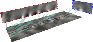
As previously mentioned, the bulk Reynolds number at each Mach number is picked to ensure approximately the same viscous Reynolds number $Re_\tau ^{*} \approx 220$, which is confirmed in table 2. Figure 4 shows the contour plot of instantaneous streamwise velocity component $u$ for all impermeable-wall LES at $y^{*} \approx 15$. Owing to the similar $Re_\tau ^{*}$, the streamwise streaks show a structural resemblance across the Mach number range being investigated, however, with a slight decrease in the spanwise size of the low-speed streaks as the Mach number increases. DNS with the same flow conditions are also performed to assess the accuracy of the LES cases; the resulting velocity contours are shown in figure 4(b,d,f). As expected, LES smooths the near-wall streak structure; this effect is more obvious in the spanwise than in streamwise direction. The Mach $6.00$ DNS case is picked for a grid convergence study due to its most stringent resolution requirement. The spatial velocity spectra in terms of streamwise and spanwise wavenumbers, $\kappa _x$ and $\kappa _z$, are shown in Appendix C, which indicates a more stringent resolution requirement in the streamwise directions. The resolutions based on the local Kolmogorov length scale are also given in table 2. Quantities reported are the maximum ratio of averaged local grid size $h = (\Delta x \Delta y \Delta z)^{1/3}$ to the local Kolmogorov length scale, i.e. $(h/\eta )_{max}$. A ratio of $h/\eta < 2.1$ is suggested (Pope Reference Pope2000) through the whole flow field for DNS study, which is a very stringent requirement. Since the impedance boundary conditions used in this work are designed to react to large-scale motions, we consider the LES resolutions to be sufficient to uncover the dynamics of flow over complex impedance walls.

Figure 4. A comparison of the instantaneous streamwise velocity component at $y^{*} \approx 15$ for LES (a,c,e) and DNS (b,d,f). The $y$-axis is pointing towards the reader. For $M_b = 6.0$, the visualization domain size was cut to match the lower Mach number cases.

Figure 5(a) shows the mean streamwise velocity $U_{TL}$, obtained with the transformation law by Trettel & Larsson (Reference Trettel and Larsson2016) and thus denoted with subscript ‘TL’. Such transformation has been shown to collapse mean velocity profiles onto the incompressible log law for channel flows at low and intermediate supersonic Mach numbers. For reference, compressible channel flow data by Ulerich (Reference Ulerich2014) ($M_b = 1.50, Re_b = 5000$) and the incompressible channel flow data from Lee & Moser (Reference Lee and Moser2015) with $Re_{\tau } \approx 180$ are also plotted. As observed in the baseline impermeable LES results, the mean velocity profile shows an overestimation of the intercept at $M_b = 1.50$; for high Mach numbers, the agreement between LES and DNS improves. Figure 5(b) to figure 5(d) present the resolved turbulent kinetic energy $k^{*} =\widetilde {u''_iu_i''}/2$ from the LES cases, along with the DNS data. Acceptable agreement is also achieved here, with the main discrepancy appearing in the peak of turbulence kinetic energy (TKE) around $y = 0.08$ in the $M_b = 1.50$ case. The overall agreement between the impermeable baseline LES and the corresponding DNS data validates the use of the impermeable LES presented herein as the base flow for the following stability analysis. From here on, only results from impermeable and permeable LES calculations will be used to investigate the dynamics of compressible turbulence over complex impedance walls.

Figure 5. Flow statistics for impermeable channel flow simulations. Mean streamwise velocity profile (a) shifted horizontally by 1.2 decade (in log scale) and turbulent kinetic energy (b–d). Data shown are: current impermeable-wall LES (black solid line), DNS (black dashed line). DNS data from Ulerich (Reference Ulerich2014) (circles), incompressible flow data from Lee & Moser (Reference Lee and Moser2015) (black filled circles), shown every four points for clarity. The reference log law $U_{TL} = 2.5\ln y^{*} + 5.5$ and law of the wall $U_{TL} = y^{*}$ are shown in red dashed lines.

6. Compressible turbulent channel flow over complex impedance

In this section, the results of permeable-wall cases are presented. The bulk Reynolds number and the bulk Mach number are chosen to be the same as the impermeable baseline simulations. The domain size for all permeable-wall cases have been shortened $L_x \times L_y \times L_z = 8 \delta \times 2 \delta \times 4 \delta$ for $M_b = 1.50$ and $M_b = 3.50$, and $L_x \times L_y \times L_z = 12 \delta \times 2 \delta \times 4 \delta$ for $M_b = 6.00$, based on the observation that the streamwise coherence length is reduced by the wall permeability. The two-point correlations of primitive variables (not shown) confirm the validity of such a choice of domain size. Grid resolutions in wall units are listed in table 3. Validation of TDIBC implementation in such a flow is provided in Appendix B.

Table 3. Grid resolutions in wall units for permeable-wall cases. Shifts in the intercept of the mean streamwise velocity profiles are reported in terms of $\Delta U_{TL}$. Top wall and bottom wall data are reported separately.

The mean streamwise velocity profiles scaled by bulk velocity are presented in figure 6(a) for permeable-wall cases. Profiles from impermeable-wall LES cases are also included as reference and shown with solid lines. Due to only the bottom wall being porous, the mean velocity profile exhibits an asymmetric pattern as compared with the impermeable-wall cases: the lower half of the channel shows a deficit in streamwise velocity while the upper channel exhibits an overshoot. The latter is merely due to the imposition of the same bulk velocity across all cases. Profiles over the bottom wall are plotted against semi-local unit $y^{*}$ and are shown in figure 6(b). Downward shifts of the scaled mean velocity profiles in the log-law region are observed at various Mach numbers, similar to the effect observed in turbulent flows over rough surfaces. For rough walls, the shift usually indicates the increase of the mean wall-shear stress (Raupach, Antonia & Rajagopalan Reference Raupach, Antonia and Rajagopalan1991; Squire et al. Reference Squire, Morrill-Winter, Hutchins, Schultz, Klewicki and Marusic2016), which is indeed observed in the current work. The shifts are reported in table 3 for all cases in terms of ${\Delta U}_{TL}$, calculated as the averaged vertical shift between two curves in the range of $y^{*} = 60 - 100$. At $M_b = 1.50$, ${\Delta U}_{TL}$ increases as the permeability increases, i.e. as $R$ is decreased, indicating a higher mean wall-shear stress. For higher Mach numbers, different resistances do not exhibit significant differences in the shift as in the low Mach number case. Note that, for $M_b = 1.50, R = 0.1$, a logarithmic trend for the upper mean velocity profile cannot be identified. The density-weighted root-mean-square (r.m.s.) wall-normal velocity fluctuations $\tilde {v}''_{rms}$ are shown in figure 7 in semi-log scale. For most of the cases, the effect of finite permeability (i.e. $R<\infty$) seems to be confined near the wall and below $y^{*} = 14$, in the buffer layer. This is not true for the high permeability case $R = 0.1$ at $M_b = 1.50$, in which $\tilde {v}''_{rms}$ sees an increase across the whole lower half-channel. In the latter case, the effects of the porous walls are globally felt by the boundary layer.

Figure 6. (a) Mean streamwise velocity profiles with various wall permeabilities normalized by bulk velocity $U_b$. (b) Mean streamwise velocity profiles based on TL-transformation in the lower half of the channel. Data shown are: $R = \infty$ (black solid line), $R = 1.00$ (black dashed dot line), $R = 0.80$ (only for $M_b = 6.00$) (black dashed line), $R = 0.50$ (black dashed line), $R = 0.10$ (black dotted line). Arrow shows direction of decreasing resistance $R$ (increasing permeability).

Figure 7. The root-mean-square (r.m.s.) wall-normal velocity fluctuations $\tilde {v}''_{rms}$ of permeable-wall cases, plotted against wall distance normalized by the semi-local unit. Arrow shows direction of decreasing resistance $R$ (increasing permeability).

To better understand the increase in mean wall shear, the instantaneous value of $\tau _w$ is monitored at the bottom wall. Figure 8 presents the probability density function (PDF) of the instantaneous wall shear extracted from the bottom wall for all cases. Values are normalized with the mean wall-shear stress over an impermeable wall (i.e. $R = \infty$) to reflect the deviation from baseline cases. For every grid point on the bottom wall, sufficient data of the instantaneous wall-shear stress $\tau _w$ are recorded over the characteristic time period – $2{\rm \pi} /\omega _{res}$ for permeable-wall cases and $\delta /U_b$ for impermeable-wall cases, which in total forms 491 520 data points for each case and guarantees the convergence of statistics. The impermeable wall results show a right-skewed PDF shape, with a peak located at the mean wall-shear stress. As the wall permeability increases, this peak shifts to the left and the PDF exhibits a longer right tail, indicating a drop in the value of the most frequently observed wall-shear stresses and an enhancement of extreme cases of positive shear stress.

Figure 8. PDF of wall-shear stress at the bottom wall normalized by the impermeable-wall value for all LES cases listed in table 3. Arrows show direction of increasing permeability.

A closer examination the flow dynamics reveals the cause of such change in the instantaneous wall-shear stress, as shown in Figure 9(a), where the $Q$-criterion (Hunt, Wray & Moin Reference Hunt, Wray and Moin1988) is used to visualize the near-wall flow structures. The contour of instantaneous wall-shear stress is also plotted. Trains of streamwise-travelling waves triggered by porosity are observed beneath the otherwise naturally present near-wall streaks and hairpin vortices. Such instability waves entail spatially oscillatory wall-shear stress and pressure patterns in the streamwise direction, and spanwise oriented vortical regions captured by the $Q$-criterion (see figure 9a,b). A zoomed view, as given in figure 9(c), clearly shows the alternation of high and low pressure regions. The high pressure regions are found to be associated with flow entrainment – the suction effect due to the outgoing wall-normal velocity, while spanwise vortical structures are regions of circulation. The impingement of the fluid onto the wall surface induces cross-flow motion as a direct effect of the fluid being expelled to the spanwise direction. This behaviour is preserved at higher Mach number $M_b = 6.00$, although with weaker strength due to the relatively high resistance $R = 0.80$. The existence of these waves affects the near-wall turbulence dynamics. As an example, they contribute to the near-wall production of TKE. We define the spectrum of the production as

(6.1)\begin{equation} \hat{P}^{k} ={-}\dfrac{1}{2} \left[ \left\langle \textrm{Re}\left\{{\widehat{\rho u'} \widehat{v'}^{{\star}}} \dfrac{\textrm{d}\tilde{u}}{\textrm{d} y}\right\} \right\rangle_{z,t} + \left \langle \textrm{Re}\left\{{\widehat{\rho v'} \widehat{u'}^{{\star}}} \dfrac{\textrm{d}\tilde{u}}{\textrm{d} y}\right\} \right\rangle_{z,t} \right], \end{equation}

where $\langle \cdot \rangle _{z,t}$ represents a averaging operator in the spanwise direction $z$ and in time $t$. Then the pre-multiplied production spectrum given as

(6.2)\begin{equation} \hat{\varPhi}_{\hat{P}^{k},x} = Re_\tau^{*} \kappa_x y \hat{P}^{k} \mu/\tau_w^{2} \end{equation}

can be plotted as a function of the streamwise wavelength $\lambda _x$ (or wavenumber $\kappa _x$) and distance away from the wall $y$. The spectra $[\hat {\varPhi }_{\hat {P}^{k},x}]$, where the bracket indicates values normalized to one, are shown in figure 10 for the highest permeability available at each Mach number. For flows with finite wall permeability, a contribution from large wavelength structure is preserved, rendered as a horizontal band of hotspots in the region $\lambda _x > 1.0, y > 0.05$. For the case $M_b = 1.50, R = 0.10$, this band is less visible due to the normalization and the high peak value in another region. For each permeable-wall case, a local peak of the production spectrum appears in the very-near-wall region with an associated wavelength. This wavelength $\lambda _x$ (scaled with the channel's half-width) is consistently equal to approximately $0.47$ for all Mach numbers, and is found to match that of the observed wave structures in the simulations. Locations of local peaks above the wall do not experience discernible variations with different permeabilities, but gradually move closer to the wall as the Mach number increases, indicating a ‘trapped’ behaviour of such wave structure at high Mach numbers. In the equivalent subsonic calculations by Scalo et al. (Reference Scalo, Bodart and Lele2015), a strong hydrodynamic response was observed and it manifests itself with the presence of large spanwise-coherent rollers, which occupy a large portion of the boundary layer (approximately 20 % of the semi-channel height). In such subsonic calculations, a much lower value of the wall resistance, $R=0.01$ was applicable to the flow, which is responsible for the strong response. As discussed in this manuscript, increasing the Mach number up to the hypersonic regime makes the adoption of resistances below $R=0.8$ impossible due to numerical blow up. In the hard incompressible limit, such as in the work by Jiménez et al. (Reference Jiménez, Uhlmann, Pinelli and Kawahara2001), such rollers are even larger, occupying the whole channel width. As the Mach number is increased past subsonic, and entering the supersonic and hypersonic regimes, the nature of the instability waves becomes more dilatational and more confined near the wall, typically below the turbulent buffer layer. The only exception is the $M_b=1.5$ case for low resistance value $R=0.1$, which resembles more the incompressible behaviour observed in Jiménez et al. (Reference Jiménez, Uhlmann, Pinelli and Kawahara2001). A turbulent channel flow with isothermal wall features an increasing wall-cooling effect as $M_b$ is increased. There is a possibility that such a phenomenon resembles the amplification of second-mode waves in cooled hypersonic boundary layers, in which an enhancement in wall cooling (or the wall-to-recovery temperature $T_{wall}/T_r$) yields a stronger instability in the hypersonic laminar boundary layer flow Fedorov (Reference Fedorov2011).

Figure 9. Visualizations of the near-wall flow dynamics for case $M_b = 6.0, R = 0.80$, presented with iso-surfaces of $Q = 90$ overlaid on: (a) instantaneous wall-shear stress contours; (b) wall pressure fluctuations. The region highlighted by the ellipse indicates a typical wave structure triggered by finite permeability, whose zoomed view is presented in (c), where red and blue dashed lines indicate locations of the plane presented in side views.

Figure 10. Contour plots of pre-multiplied production spectrum $\hat {\varPhi }_{\hat {P}^{k},x}$ as a function of streamwise wavelength $\lambda _x$ and distance away from the wall $y$. For each Mach number, the cases with an impermeable wall (first row) and with the highest wall permeability (second row) are presented. The location of the local peak due to finite permeability is labelled with a symbol.

The impedance boundary condition defines the phase and amplitude relation between pressure and velocity signals at the wall. This concept could be extended to wavenumber space, in order to relate it to structural features of turbulence, in which one can also define an impedance $\hat {Z}(\kappa )$, or its inverse, admittance $\hat {Y}(\kappa )$, as

(6.3)\begin{equation} \hat{Y}(\kappa;y) = \bar{\rho}(y) \bar{a}(y) \hat{v}(\kappa;y)/\hat{p}(\kappa;y), \end{equation}

where $\kappa$ can take on values of $\kappa _x$ or $\kappa _z$ denoting streamwise and spanwise wavenumbers, respectively. A plot of $||\hat {Y}(\kappa _x)||$ is shown in figure 11 for $M_b = 1.50$ with various permeabilities, at five $y$ locations below a quarter of half-channel height, i.e. $0.25\delta$. Note that the impermeable-wall case yields zero admittance on the wall because of the no-penetration condition, thus cannot be presented on a log-scale plot. Clearly, the effect of porosity-induced pressure/velocity phasing penetrates towards the channel centre for increasing wall permeability. The near-wall admittance peaks at the wavenumber corresponding to wave structures previously reported (the wavelength $\lambda _x = 0.47$). This then offers the opportunity to connect turbulence structure analysis and impedance boundary conditions. For typical turbulence structures residing in turbulent boundary layers or turbulent channel flows, their convective speed $U_c$ and wavelength $\lambda _x$ have obtainable scalings based on the semi-local unit for compressible flows (or the plus unit for incompressible flows). With this information, it would then be possible to construct a wall admittance $\hat {Y}(\omega )$ that resonates at $\omega _{res} = U_c\kappa _x$, where $U_c$ and $\kappa _x$ are the associated convective speed and wavenumber of the near-wall turbulent structure. In such a way, the boundary condition is then linked to the characteristic wavenumber (wavelength) of dominating structures in boundary layer type flows.

Figure 11. The magnitude of acoustic admittance as a function of streamwise wavenumber $k_x$ for $M_b = 1.50$ with various wall permeabilities. Values of admittance are plotted at five $y$-location below a quarter of channel half-height. The impermeable-wall case has zero admittance on the wall due to the no-penetration condition and thus cannot be presented on a log-scale figure.

7. Linear stability analysis

In this section, temporal linear stability analysis (LSA) is performed at all flow conditions with various bottom wall permeabilities. To perform the analysis, the Navier–Stokes equations are linearized by decomposing each instantaneous variable into a base $\bar {\phi }$ and a fluctuation $\phi '$ component via

(7.1a,b)\begin{equation} \phi = \bar{\phi} + \phi', \quad |\phi'| \ll |\bar{\phi}|. \end{equation}

For channel flow, the base variable is independent of time while the small perturbation is assumed to have the harmonic form

(7.2)\begin{equation} \phi' = \hat{\phi}(y)\textrm{e}^{{\rm i}(\alpha x - \varOmega t)}, \end{equation}

where ${\rm i} = \sqrt {-1}$; $\alpha$ and $\varOmega$ are the streamwise wavenumber and angular frequency, respectively. Note that the symbol ${\rm i}$ also serves as the index in the Einstein notation, but only when it appears as a subscript. The angular frequency $\varOmega$ is the opposite of $\omega$ as defined in the TDIBC formulation, favouring the convention used in wave propagation problems. The complex amplitude $\hat {\phi }$ is allowed to vary with distance away from the bottom wall. Polynomials at Gauss–Lobatto–Chebyshev points are used to approximate the solution and the problem is reformulated into a generalized eigenvalue problem (GEP) $\boldsymbol{\mathsf{A}}\boldsymbol {{\varPhi }} = \varOmega \boldsymbol{\mathsf{B}}\boldsymbol {{\varPhi }}$, with the solution vector given by $\boldsymbol {{\varPhi }} = \{ \hat {u}, \hat {v}, \hat {p}, \hat {T}\}^{\boldsymbol {T}}$. The linearized governing equations are included in Appendix D, along with code verification against results in the existing literature. Reynolds-averaged flow quantities from the impermeable-wall LES simulations in § 5 are used as the base flow profiles. To account for the background turbulent mixing, turbulent viscosity $\bar {\mu }_{{turb}}$ is added to the total viscosity in LSA, neglecting its perturbation ${\mu }'_{{turb}}$. The turbulent viscosity can be obtained either by fitting an analytical model to a given flow condition, or by direct calculation via $\bar {\mu }_{{turb}} = \overline {\rho u''v''}/(\textrm {d}U/{\textrm {d} y})$. For the first method, Cess (Reference Cess1958) has proposed an analytical form of $\mu _{turb}$ as a function of Reynolds number and pressure gradient in an incompressible turbulent pipe flow, which has been later adapted by Reynolds & Tiederman (Reference Reynolds and Tiederman1967) and Reynolds & Hussain (Reference Reynolds and Hussain1972) for incompressible channel flow (see also Del Alamo & Jimenez Reference Del Alamo and Jimenez2006; Pujals et al. Reference Pujals, García-Villalba, Cossu and Depardon2009; Rinaldi et al. Reference Rinaldi, Patel, Schlatter and Pecnik2017; Sebastian et al. Reference Sebastian, Marx and Fortuné2019). The second method is more straightforward, but leads to error propagation due to the division operation. Nevertheless, for this study, the latter is used. Smoothing functions are applied near the channel centre where $\mu _{turb}$ is affected most by such an error. Then, the smoothed $\mu _{turb}$ is used in the mean streamwise momentum equation to re-obtain $U$ through integration, which is compared to the Reynolds-averaged results from the simulations to ensure the validity of the calculated $\mu _{turb}$.

The following boundary conditions are used in the LST study. No-slip and isothermal wall conditions lead to homogeneous Dirichlet boundary conditions for perturbations in temperature and streamwise velocity, that is, $\hat {u} = 0$ and $\hat {T} = 0$ at both walls. A non-homogeneous Neumann condition is used for pressure by applying the linearized wall-normal momentum equation (D7) at the wall grid point. Application of the impedance boundary condition with the adopted three-parameter model results in nonlinearity because of the $\varOmega ^{-1}$ dependence in the spring-like acoustic reactance term, and thus imposes difficulties in numerics. To circumvent this issue, the method suggested by Malik (Reference Malik1990) is used by introducing an auxiliary variable $\hat {\tilde {v}} = \varOmega \hat {v}$, extending the original solution vector to $\boldsymbol {{\varPhi }} = \{ \hat {u}, \hat {v}, \hat {p}, \hat {T}, \hat {\tilde {v}}\}^{\boldsymbol {T}}$. The increase in computational cost is acceptable since only one more variable is added. Homogeneous Dirichlet condition is applied to $\hat {v}$ for walls with zero permeability. For temporal linear stability problems, the wavenumber $\alpha$ is required as an input. Throughout this study, the wavenumber is fixed to $\alpha = 2{\rm \pi} /\lambda _x$, with $\lambda _x=0.47$, approximately matching the wavenumber of wave structures observed in the permeable-wall LES simulations. It has been pointed out by Hu & Zhong (Reference Hu and Zhong1997) that spurious modes will appear in the GEP results when performing LST study, which can be easily identified via a grid convergence study since the locations of spurious modes in eigenspace are usually grid dependent. By using polynomial degrees in the range $N = 200$, 300, 400, 500 and comparing the eigenvalue spectrum, $N = 300$ is found to sufficiently resolve the spectrum in the region of interest for all Mach numbers. For all flow conditions, 20 values of $R = \{0.10,0.20, \dots , 1.0, 2.0, \dots , 10.0, \infty \}$ are selected to conduct the study, where $R = \infty$ corresponds to the impermeable-wall case. Figure 12 shows the spectrum of complex wave speed $c = \varOmega /\alpha = c_r + \textrm {i}c_i$ scaled by bulk Mach number $M_b$. The trajectory of the mode affected by wall permeability is highlighted in red, while the black symbols represent modes in an impermeable-wall case, whose locations remain almost fixed when $R$ varies.

Figure 12. Eigenspectrum of a compressible turbulent channel flow for various bottom wall permeabilities for all bulk Mach numbers. The input wavenumber is taken as $\alpha = 2{\rm \pi} /\lambda _x$ where $\lambda _x=0.47$ is taken from the permeable-wall LES. The IBC resistance is varied in the range $R = \{0.10,0.20, \dots , 1.0, 2.0, \dots , 10.0, \infty \}$. The red dashed line represents the trajectory of the mode affected by porosity with the arrow showing the direction of increasing permeability (or decreasing $R$). The filled black diamonds indicate scaled eigenvalues that do not vary with $R$, while red unfilled diamonds and circles represent the beginning ($R = \infty$) and the end ($R = 0.10$) of the trajectory of the mode affected by permeability, respectively.

Even with finite permeability, the overall spectrum retains the typical three-branch shape: a vertical stem roughly located at $Re\{c/M_b\} = 1$ indicating modes convecting at the bulk speed; two tilted branches that have zero or negative imaginary part, representing neutrally stable or damped modes. Introducing turbulent viscosity results in a strong damping effect on the modes belonging to left and right branches. A red dashed line highlights the trajectory of the mode made unstable by porosity, with a circle indicating the case with lowest resistance $R = 0.10$, i.e. highest wall permeability, and a diamond indicating the impermeable limit $R = \infty$. At any given Mach number, increasing the wall permeability (or decreasing $R$) increases the growth rate of this mode, gradually moving it towards the unstable region (upper half-plane). Figure 13(a) collects all trajectories of the permeability-triggered mode from different Mach numbers and wavenumbers. For unstable modes, higher Mach number favours a higher growth rate, but lower scaled phase velocity at a given resistance $R$. The points at which each trajectory crosses zero, defined as critical resistance $R_{cr}$, are extracted and shown in figure 13(b). A sub-linear dependence of $R_{cr}$ on $M_b$ is observed, which indicates that higher Mach numbers require low permeability to trigger such a type of instability.

Figure 13. (a) Trajectory of an eigenmode tracked in red in figure 12 re-proposed here for all Mach numbers and a streamwise wavelength of $\lambda _x=0.47$, as observed in the permeable-wall LES. Arrow shows the direction of increasing permeability (or decreasing $R$). (b) The critical resistance $R_{cr}$ (unfilled circles) below which the mode in (a) becomes unstable as a function of bulk Mach number $M_b$.

It should be noted that for hypersonic bulk Mach numbers of $M_b = 6.0$ the linear stability predicts no unstable modes for values of resistance above $\sim$0.77; however, a modal instability can still be detected in permeable-wall hypersonic LES calculations at $R = 0.8$. The latter is suppressed by increasing the resistance further to $R=1.0$ indicating that the effective critical resistance value for hypersonic conditions is in the range $R_{cr} = 0.8 - 1.0$. Such a range of critical values is still quite narrow compared with typical values of wall resistance observed in porous walls used for hypersonic applications, which can exceed $R=10$ (Sousa et al. Reference Sousa, Patel, Chapelier, Wartemann, Wagner and Scalo2019) over a broad range of ultrasonic frequencies.

The angular frequency associated with the tracked mode can be obtained from the simple relation $\varOmega _r = \alpha c_r$, where $c_r$ is the real part of phase velocity. For values of $R$ available in three-dimensional simulations, table 4 lists the scaled phase velocity $c_r/M_b$ and normalized angular frequency $\varOmega _r/\varOmega _\text {res}$ obtained from LST. A near-unitary value of $\varOmega _r/\varOmega _{res}$ indicates that the frequency of the temporally growing mode is very close to the resonating frequency of the IBC, at which the flow is excited the most. The eigenfunctions of $\hat {p}$ and $\hat {v}$ of the mode tracked in figure 12 are shown in figure 14. Only modes with $R < R_{cr}$ are shown. It is apparent that most of the perturbation energy is trapped in the near-wall region, consistent with the trapped wave pattern observed in the simulations as shown in figure 9. Figure 15 shows the contour plot of the pressure mode from LST prediction and the pressure fluctuation extracted from filtered LES results for the lowest resistance available at each Mach number. The latter contour plot was obtained by performing an average in the $z$-direction in a small box that contains the whole wave structure. A good resemblance is obtained in the pressure fluctuations between LST results and full-scale simulations. Top–down views of the contour plot of the pressure fluctuation on the wall are provided for the corresponding cases in figure 16. In fact two types of wave structures are observed at a fixed Mach number with different wall permeabilities, clearly with different wavelengths (it is difficult to observe these structures in the cases of $M_b = 1.50$). In the impermeable-wall simulations, these waves are associated with the ‘footprint’ of large streamwise scales and can still be observed in the permeable-wall simulations. With the finite wall impedance, these structures co-exist with waves with different length scale, triggered by the response of the permeable walls.

Figure 14. Scaled real part of the pressure and velocity eigenfunctions associated with the tracked mode for resistance values below $R_{cr}$ at each Mach number. For clarity, only values of following $R$ are selected to plot: $R = 0.10$ (black dotted line), $R = 0.30$ (black dotted line), $R = 0.50$ (black dotted line), $R = 0.70$ (black solid line).

Figure 15. Contour of unstable pressure mode (a–c) from LST and pressure fluctuations near the wall extracted from the LES (d–f). Pressure fields from the three-dimensional simulations are first filtered with a bandpass Butterworth filter, keeping only the wavelengths in the range $[0.35, 0.5]$. A $z$-plane average is then performed on the filtered pressure field among planes that cut through the wave structures. Values are normalized with the maximum amplitude of pressure fluctuation. Positive and negative levels are shown with solid and dashed lines, respectively. Note that for the linear stability result at $M_b = 6.00$, the highest data point of $R$ below $R_{cr}$ is $0.70$ instead of $0.80$ used in the simulation.

Figure 16. Top–down view of the pressure fluctuations on the bottom wall. Left column shows the LES impermeable-wall results, right column shows the permeable-wall cases presented in figure 15, with the white box showing the region where filtered pressure fields are extracted.

Table 4. The scaled phase velocity and associated angular frequency of the tracked mode for values of resistance also investigated with LES. The angular frequency is normalized with the resonating frequency $\varOmega _{res}$.

Although a good match is achieved between LST and simulations, one must keep in mind that temporal LST is meant to predict the stability of a linearly growing perturbation. In contrast, instability observed in the three-dimensional simulations has reached a saturation state due to the interaction between near-wall turbulence and acoustic response from the wall. Hence, the physical process that LST is predicting is the onset state of a complex IBC applied to the turbulent field developed over an impermeable wall.

The complex velocity field due to the instability is further decomposed into dilatational $\hat {\boldsymbol {v}}_d$ and solenoidal part $\hat {\boldsymbol {v}}_s$, i.e. $\hat {\boldsymbol {v}} = \hat {\boldsymbol {v}}_d + \hat {\boldsymbol {v}}_s$. To account for the contribution of the two components, the ratio of the integrated norm

(7.3)\begin{equation} \dfrac{E_d}{E_s} = \dfrac{\displaystyle\int_0^{2} |\textrm{Re}\{\hat{\boldsymbol{v}}_d \textrm{e}^{-\alpha c}\}|^{2} \,{\textrm{d} y}}{\displaystyle\int_0^{2} |\textrm{Re}\{\hat{\boldsymbol{v}}_s\textrm{e}^{-\alpha c}\}|^{2} \,{\textrm{d} y}} \end{equation}

is evaluated for the normal velocity component for cases with $R < R_{cr}$ for all Mach numbers. Results are shown in Figure 17 for wavenumbers (wavelengths) associated with those appearing in LES. At each Mach number, the dilatational field occupies a discernible amount of energy once the instability is triggered, and is gradually weakened as permeability increases. The perturbed flow fields exhibit a more hydrodynamic nature as the response of the impedance wall to the overlying turbulent field becomes stronger. In addition, the same (non-dimensionalized) permeability tends to yield a perturbed field with higher portion of dilatational energy at higher Mach number.

Figure 17. Ratio of the integrated norm of dilatational part $\hat {\boldsymbol {v}}_d$ and solenoidal part $\hat {\boldsymbol {v}}_s$ of the perturbed field, $E_d/E_s$, defined in (7.3) vs the inverse of the wall resistance. Results are obtained by applying the Helmholtz–Hodge decomposition to the velocity eigenfunctions of the unstable mode. Only resistance values below $R_{cr}$ are shown here, with $\lambda _x =0.47$.