


1. Introduction
Studying the fundamental interactions of vortices helps us understand the behaviour of the complicated flows which can be encountered in nature. A simple example of an interaction is two-dimensional vortex merging, which is a well-studied phenomenon in fluid mechanics. For a general review of the dynamics and instabilities of vortex pairs, see e.g. Leweke, Le Dizès & Williamson (Reference Leweke, Le Dizès and Williamson2016). It is sometimes possible to observe vortex merging visually in experiments and numerical simulations, but it can be difficult to give an accurate mathematical description of the merging process. Early studies of vortex merging mainly focus on merging in inviscid fluids where vortices are defined as vortex patches with constant vorticity (Overman & Zabusky Reference Overman and Zabusky1982; Dritschel Reference Dritschel1985). The jump of vorticity across vortex boundaries is advected by the velocity field and the problem effectively becomes one-dimensional. This approach, known as contour dynamics, was originally proposed by Deem & Zabusky (Reference Deem and Zabusky1978). The conservation of vorticity ensures that the fluid will be divided into regions of uniform vorticity for all time and, in principle, merging is never possible. Dritschel (Reference Dritschel1986) overcomes this issue by applying contour surgery, which is an algorithm allowing two contours enclosing the same uniform vorticity to merge into one if they are close enough together. In this study, we will address the problem rigorously in a viscous setting. We identify vortices by the widely used  $Q$-criterion (Hunt, Wray & Moin Reference Hunt, Wray and Moin1988). In its general form, Q is defined as the following measure of stretching relative to rotation,
 \begin{equation}
Q = \tfrac{1}{2}(\|\boldsymbol{\Omega}\|^2 - \|\boldsymbol{\mathsf{S}}\|^2),
\end{equation}
\begin{equation}
Q = \tfrac{1}{2}(\|\boldsymbol{\Omega}\|^2 - \|\boldsymbol{\mathsf{S}}\|^2),
\end{equation}
where  $\boldsymbol{\mathsf{S}}=\frac{1}{2}(\nabla \mathbf{u}+\nabla \mathbf{u}^T)$ is the symmetric strain rate tensor,
  $\boldsymbol{\Omega}=\frac{1}{2}(\nabla \mathbf{u}-\nabla \mathbf{u}^T)$ is the skew-symmetric vorticity tensor and
  $\|\boldsymbol{\mathsf{X}}\|=\sqrt{\text{tr}(\boldsymbol{\mathsf{X}} \boldsymbol{\mathsf{X}}^T)}$. The Q-criterion defines a vortex as a region with positive Q-value. In two dimensions,
  $Q$ simplifies to the determinant of the velocity gradient tensor
  $\boldsymbol {\nabla } \boldsymbol {u}$ and a vortex is therefore defined as a region where
 \begin{equation} Q(x,y)=\text{det}(\boldsymbol{\nabla} \boldsymbol{u}(x,y))>0. \end{equation}
 In this paper, we present a complete topological analysis of the merging of  $Q$-vortices in the core growth model. The main result of our analysis is that the merging process can be divided into three different regimes depending on the strength ratio of the vortices. For sufficiently high strength ratio, the weakest vortex is supressed by the strong vortex, and no merging as such occurs. For lower strength ratios, there are two different bifurcation sequences leading to merging. The core growth model has previously been used to study vortex merging by Jing, Kanso & Newton (Reference Jing, Kanso and Newton2012) and Andersen et al. (Reference Andersen, Schreck, Hansen and Brøns2019). In the following section we review the model and show that it allows us to write an analytical expression for
  $Q$ depending on two parameters, the strength ratio of the two vortices and the time.
We monitor the vortex interactions by looking for bifurcations of the curves bounding the vortices, the level curves  $Q(x,y)=0$. Bifurcations occur when singular points appear on these curves. An analysis of all possible perturbations of a given degenerate pattern tells us what we might expect when a given number of parameters are allowed to vary. When only a single parameter is varied, the bifurcations that occur in a robust way are referred to as having codimension one. We have already formulated a complete codimension one theory in earlier studies, see Nielsen et al. (Reference Nielsen, Heil, Andersen and Brøns2019) or the brief summary in § 3. Our previous study includes an analysis of a single codimension two phenomenon, but as the core growth model has two free parameters, it is necessary to extend the existing theory with an analysis of another codimension two bifurcation. This further development of the theory can be found in § 3.1. The core growth model has a built-in symmetry that may lead to a special type of codimension two bifurcation; this case is analysed in § 3.2. We compare the results for the core growth model with Navier–Stokes simulations in § 4.1, and find good agreement for low values of the Reynolds number. An analysis of the topological structure of vortex pairs is inextricably linked to the way we choose to define vortices mathematically. There are many definitions of vortices available in the literature, see Zhang et al. (Reference Zhang, Liu, Xian and Du2018) for a review. To our knowledge, this is the first study to analyse vortex pair interactions based on the topology of the
  $Q$-criterion. Andersen et al. (Reference Andersen, Schreck, Hansen and Brøns2019) have previously studied vortex merging from a topological point of view with vortices defined as local extrema of vorticity. This method identifies a vortex by a feature point that does not provide any information about the shape or size of the vortex. Applying the
  $Q$-criterion might therefore provide some opportunities for a more elaborate analysis. In § 5 we comment on the importance of the vortex criterion.
2. The core growth model
We consider an incompressible fluid in an unbounded two-dimensional domain governed by the Navier–Stokes equations. In terms of the vorticity, the Navier–Stokes equations can be written as the vorticity transport equation,
 \begin{equation} \dfrac{\partial \omega}{\partial t}={-}\boldsymbol{u}\boldsymbol{\cdot} \boldsymbol{\nabla} \omega + \nu \Delta \omega, \end{equation}
where  $\omega$ is the vorticity,
  $\nu$ is the kinematic viscosity and
  $\boldsymbol {u}$ is the fluid velocity. One of the very few known analytic solutions to (2.1) is the Lamb–Oseen vortex (Saffman Reference Saffman1992). In polar coordinates
  $(r,\theta)$ the vorticity and velocity components are
 \begin{equation} \left.\begin{gathered} \omega(r,\theta,t)=\dfrac{\varGamma}{{\rm \pi} \sigma(t)^2} \exp({-r^2/\sigma(t)^2}), \quad u_\theta(r,\theta,t)=\dfrac{\varGamma}{2 {\rm \pi}r}( 1-\exp({-r^2/\sigma(t)^2}) ), \\ u_r(r,\theta,t)=0, \end{gathered}\right\} \end{equation}
with
 \begin{equation} \sigma(t)=\sqrt{4\nu t}. \end{equation}
The Lamb–Oseen vortex is the solution corresponding to a single point vortex with strength  $\varGamma$ as initial condition. The vorticity field
  $\omega$ is initially concentrated at the origin and diffuses as a Gaussian distribution. For multiple point vortices as the initial condition, an analytic solution is not available and one would generally refer to numerical simulations of the vorticity transport equation. Instead, we investigate the synthetic flow predicted by the core growth model, also known as the multi-Gaussian model (Jing, Kanso & Newton Reference Jing, Kanso and Newton2010; Kim & Sohn Reference Kim and Sohn2012; Andersen et al. Reference Andersen, Schreck, Hansen and Brøns2019). The model assumes that the vorticity of each initial point vortex diffuses symmetrically as an isolated Lamb–Oseen vortex and the centres of the Gaussian vortices move in the velocity field induced by the other diffusing vortices. For two Gaussian vortices, initially centred at
  $(-d,0)$ and
  $(d,0)$, one can deduce (Kim & Sohn Reference Kim and Sohn2012) that the distance between the centres of the two Gaussian vortices is conserved and the vortices rotate around the a stationary centre of vorticity
 \begin{equation} (x_{cv},y_{cv})=\left(\dfrac{d(\varGamma_2-\varGamma_1)}{\varGamma_1+\varGamma_2},0\right), \end{equation}
with the same time-dependent angular velocity
 \begin{equation} \frac{\textrm{d}\phi(t)}{\textrm{d}t}=\dfrac{\varGamma_1+\varGamma_2}{2{\rm \pi}(2d)^2}(1-\exp({-(2d)^2/\sigma^2})). \end{equation}
 We notice that the angular velocity tends to zero as  $\nu$ or
  $t$ increases. By integrating
  ${\textrm {d}\phi (t)}/{\textrm {d}t}$ in time we obtain the direction angle as a function of time
 \begin{equation} \phi(t)=\dfrac{\varGamma_1+\varGamma_2}{2{\rm \pi}(2d)^2\nu}\left(\frac{\sigma^2}{4}- \frac{\sigma^2}{4}\exp({-(2d)^2/\sigma^2}) +d^2\int_{(2d)^2/\sigma^2}^\infty\,\dfrac{\textrm{e}^{{-}s}}{s}\,\textrm{d}s\right). \end{equation}
 We notice that the angular velocity and the direction angle depend on the total of vortex strength  $\varGamma _1+\varGamma _2$ and the distance between the vortices, not on the strength ratio. The positions of the two Gaussian vortex centres
  $(x_1(t),y_1(t))$,
  $(x_2(t),y_2(t))$ are given by (2.6), i.e.
 \begin{gather} \begin{pmatrix} x_1(t)\\y_1(t) \end{pmatrix}=\begin{pmatrix} d-x_{cv} \end{pmatrix}\begin{pmatrix} \cos \phi(t)\\\sin \phi(t) \end{pmatrix}+\begin{pmatrix} x_{cv}\\0 \end{pmatrix}, \end{gather}
 \begin{gather}\begin{pmatrix} x_2(t)\\y_2(t) \end{pmatrix}={-}\begin{pmatrix} d+x_{cv} \end{pmatrix}\begin{pmatrix} \cos \phi(t)\\\sin \phi(t) \end{pmatrix}+\begin{pmatrix} x_{cv}\\0 \end{pmatrix}. \end{gather}
Since the core growth model evolves as a superposition of two Lamb–Oseen vortices, the vorticity field is given as
 \begin{equation} \omega(x,y,t)=\dfrac{\varGamma_1}{{\rm \pi} \sigma^2} \exp({-d_1^2/\sigma^2})+\dfrac{\varGamma_2}{{\rm \pi} \sigma^2} \exp({-d_2^2/\sigma^2}), \end{equation}
where
 \begin{gather} d_1^2=(x-x_1(t))^2+(y-y_1(t))^2, \end{gather}
 \begin{gather}d_2^2=(x-x_2(t))^2+(y-y_2(t))^2. \end{gather}
By solving the Poisson equation  $\omega = -\Delta \psi$ we obtain the following streamfunction in the core growth model
 \begin{align} \psi(x,y,t)={-}\dfrac{\varGamma_1}{4{\rm \pi}}\left(\ln\left(d_1^2\right)+\int_{d_1^2/\sigma^2}^\infty \,\dfrac{\textrm{e}^{{-}s}}{s}\,\textrm{d}s\right)-\dfrac{\varGamma_2}{4{\rm \pi}}\left(\ln\left(d_2^2 \right)+\int_{d_2^2/\sigma^2}^{\infty}\,\dfrac{\textrm{e}^{{-}s}}{s}\,\textrm{d}s\right). \end{align}
 The core growth model is not an exact solution to the vorticity transport equation in (2.1). However, by inserting the synthetic flow into the equation, we can evaluate the error we make when using the core growth model. From (2.7), (2.8), (2.9) and (2.12) all three terms in the vorticity transport equation can be expressed analytically and by evaluating the limit as  $\nu \to \infty$ we obtain for a fixed
  $t$ that
 \begin{equation} \partial_t\omega -\nu \Delta \omega + \boldsymbol{u}\boldsymbol{\cdot} \boldsymbol{\nabla} \omega=\frac{(\varGamma_1^2-\varGamma_2^2)yd}{32{\rm \pi}^2\nu^3t^3}+{O} \left(\frac{1}{\nu^4}\right)\quad \text{as}\ \nu \to \infty, \end{equation}
which implies that the core growth model will be accurate for the viscosity going to infinity, i.e. for the Reynolds number going to zero. This will be confirmed by numerical computations in § 4.3. The quality of the approximation will necessarily depend on the value of the fixed  $t$. For a smaller
  $t$ value, a lower Reynolds number is required to achieve the given accuracy. Part of the purpose of this study is to establish an upper limit of the Reynolds number under which it is reasonable to use the core growth model instead of numerically solving the Navier–Stokes equation. It is worth noting that Gallay (Reference Gallay2011) proved that on a fixed time interval the solution to the vorticity transport equation, with point vortices as initial conditions, converges uniformly in time to a superposition of Lamb–Oseen vortices as
  $\nu \to 0$. Since the core growth model has point vortices as the initial condition, Gallay's result indicates that the model will be relatively accurate also in weakly viscous flow. The model has previously been studied for
  $Re = (|\varGamma_1|+|\varGamma_2|)/(2\nu) \gg 1$, see Jing et al. (Reference Jing, Kanso and Newton2012) for an example.
For simplicity, the core growth model will be studied in a co-rotating frame, such that the centres of the Gaussian vortices are fixed at the initial positions. For a given time  $t$, the transformation from the co-rotating to the initial frame is determined by a rigid rotation with the angle
  $\phi (t)$ around the centre of vorticity. This guarantees that the topology of the vorticity field, the streamfunction and hence also the
  $Q$-field are unchanged when studied in the co-rotating frame. To analyse the core growth model for all possible combinations of vortex strengths and displacements, we introduce the following dimensionless variables (denoted with
  $\sim$),
  $\tilde {x}= x/d$,
  $\tilde {y}= y/d$,
  $\tilde {\omega }= \omega d^2/\varGamma _2$,
  $\tilde {\sigma }= \sigma /d$,
  $\tilde {\psi }= \psi d^2/\varGamma _2$ and
  $\tilde {\psi }= \psi /\varGamma _2$. For simplicity, we drop the tildes from now on. In the co-rotating coordinate system the dimensionless vorticity and streamfunction for the core growth model become
 \begin{equation} \omega(x,y,\alpha,\sigma)=\dfrac{\alpha}{{\rm \pi} \sigma^2} \exp\left({-\frac{(x+1)^2+y^2}{\sigma^2}}\right)+\dfrac{1}{{\rm \pi} \sigma^2} \exp\left({-\frac{(x-1)^2+y^2}{\sigma^2}}\right), \end{equation}
and
 \begin{align}
\psi(x,y,\alpha,\sigma)&={-}\dfrac{\alpha}{4{\rm \pi}}\left(\ln((x+1)^2+y^2)+
\int_{{((x+1)^2+y^2)}/{\sigma^2}}^{\infty}
\dfrac{\textrm{e}^{{-}s}}{s}\,\textrm{d}s\right)\nonumber\\
&\quad -\dfrac{1}{4{\rm \pi}}\left(\ln((x-1)^2+y^2)+\int_{({(x-1)^2+y^2})/{\sigma^2}}^\infty
\dfrac{\textrm{e}^{{-}s}}{s}\,\textrm{d}s\right),
\end{align}
\begin{align}
\psi(x,y,\alpha,\sigma)&={-}\dfrac{\alpha}{4{\rm \pi}}\left(\ln((x+1)^2+y^2)+
\int_{{((x+1)^2+y^2)}/{\sigma^2}}^{\infty}
\dfrac{\textrm{e}^{{-}s}}{s}\,\textrm{d}s\right)\nonumber\\
&\quad -\dfrac{1}{4{\rm \pi}}\left(\ln((x-1)^2+y^2)+\int_{({(x-1)^2+y^2})/{\sigma^2}}^\infty
\dfrac{\textrm{e}^{{-}s}}{s}\,\textrm{d}s\right),
\end{align}where
 \begin{equation} \alpha=\frac{\varGamma_1}{\varGamma_2}, \quad \sigma^2=\frac{4\nu t}{d^2} \end{equation}
are the strength ratio of the two vortices and a dimensionless time variable, respectively. As a result, the Gaussian vortices are fixed at  $(-1,0)$,
  $(1,0)$. As described in the introduction, we will analyse the topological bifurcations of vortex pair interactions by applying the
  $Q$ criterion. Using (2.15), a closed analytical expression for
  $Q$ in the co-rotating frame can be directly computed from
 \begin{equation} Q(x,y,\alpha,\sigma)=\left(\dfrac{\partial^2\psi}{\partial x^2}\right)\left(\dfrac{\partial^2\psi}{\partial y^2}\right)-\left(\dfrac{\partial^2\psi}{\partial x\partial y}\right)^2. \end{equation}
In § 4.1, we will analyse the zero level curves of this function in detail. We note that the model has a built-in symmetry. The  $x$-axis is a line of symmetry in the streamfunction and hence
 \begin{equation} Q(x,-y,\alpha,\sigma)=Q(x,y,\alpha,\sigma) \end{equation}
for all values of  $x,y,\alpha$ and
  $\sigma$. Furthermore, it follows from (2.15) that
 \begin{equation} Q(x,y,\alpha,\sigma)=\alpha Q\left({-}x,y,\dfrac{1}{\alpha},\sigma\right), \end{equation}
which makes it sufficient to investigate the topological bifurcations of the zero level curves of  $Q$ for
  $|\alpha |\geqslant 1$.
3. Bifurcation theory for  $Q$-vortices

A general characterization of zero level curves of  $Q$ may be applied to any flow situation, regardless of whether it arises from the core growth model or the Navier–Stokes equations. Nielsen et al. (Reference Nielsen, Heil, Andersen and Brøns2019) show that there are two types of robust one-parameter bifurcations of the level curves
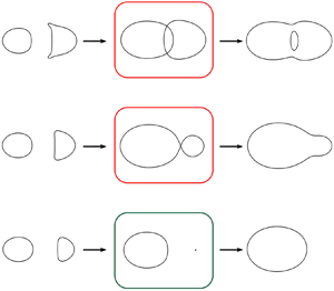
  $Q=0$, the authors denoted these as a pinching and a punching bifurcation, see figure 1. The bifurcations occur when
 \begin{equation} Q=0, \quad \partial_x Q=0,\quad \partial_y Q=0, \end{equation}
under the non-degeneracy conditions
 \begin{equation} \partial_t Q\neq0 \end{equation}
and
 \begin{equation} \boldsymbol{\mathsf{H}}^Q=\begin{pmatrix} \partial_{xx} Q & \partial_{xy} Q\\ \partial_{xy} Q & \partial_{yy} Q \end{pmatrix}\ \text{is non-singular}. \end{equation}
Here,  $t$ denotes a free parameter. A pinching (punching) bifurcation occurs when
  $\boldsymbol{\mathsf{H}}^Q$ is indefinite (definite), and the direction of the bifurcation depends on the sign of
  $\partial _t Q$. A pinching bifurcation is the splitting or merging of two vortices while a punching bifurcation is the creation or disappearance of a single vortex.

Figure 1. Illustration of the local changes in the structure of the  $Q=0$ contour curves during a (a) pinching and a (b) punching bifurcation. The bifurcation states are depicted in red and green boxes. The dashed lines in (a) show an example of a possible global structure during a pinching bifurcation. Note that the empty left panel in (b) illustrates that there are no
  $Q=0$ contour curves.
In general there is no simple connection between the vorticity  $\omega$ and the
  $Q$-value. If we consider an incompressible fluid at a point
  $(x,y)$ with
  $\omega =0$, we notice, however, that
 \begin{equation} Q=\partial_xu\partial_yv-\partial_yu\partial_xv={-}(\partial_xu)^2-(\partial_yu)^2. \end{equation}
Since  $Q\leqslant 0$, we conclude that a point with zero vorticity will always be located outside or on the boundary of a
  $Q$-vortex. By continuity it is therefore impossible to have points with opposite signs of vorticity in the interior of a single vortex. Hence, two vortices can only merge in a pinching bifurcation if they have the same sign of vorticity in the interior.
3.1. Theoretical description of codimension two bifurcation
A flow may depend on several parameters, such as the Reynolds number or a parameter that determines the initial geometry. In this section, we consider a flow described as a smooth system depending on two parameters,  $t$ and
  $r$. In this setting, the two generic types of one-parameter bifurcations occur when crossing a one-dimensional bifurcation curve in the
  $(t,r)$ parameter space. A codimension two point on one of these bifurcation curves is a point where both parameters are required to take on particular values, so that one of the non-degeneracy conditions in (3.2) or (3.3) are violated. The codimension two bifurcation where
  $\partial _tQ=0$ is analysed in detail in previous studies (Nielsen et al. Reference Nielsen, Heil, Andersen and Brøns2019). In this section, we will analyse the other bifurcation phenomenon that occur when
  $\boldsymbol{\mathsf{H}}^Q$ is singular with 0 as a simple eigenvalue. For simplicity, we choose a coordinate system such that the bifurcation point is located at
  $(x, y, t, r) = (0, 0, 0, 0)$ and
  $\boldsymbol{\mathsf{H}}^Q$ is a diagonal matrix. We consider a bifurcation point characterized by the following set of degeneracy conditions
 \begin{equation} Q_0=0, \quad \partial_x Q_0=0, \quad \partial_y Q_0=0 \end{equation}
and
 \begin{equation} \boldsymbol{\mathsf{H}}^Q_0=\begin{pmatrix} \partial_{xx} Q_0 & \partial_{xy} Q_0 \\ \partial_{xy} Q_0 & \partial_{yy} Q_0 \end{pmatrix} = \begin{pmatrix} 0 & 0 \\ 0 & \lambda \end{pmatrix}, \end{equation}
where subscript  $0$ is used to denote an evaluation at the bifurcation point
  $(x,y,t,r) =(0,0,0,0)$ and
  $\lambda$ is a non-zero parameter. To characterize the structure of the bifurcation curves at the bifurcation point we assume some regularity in the form of the following set of non-degeneracy conditions
 \begin{equation} \partial_t Q_0\neq0, \quad \partial_r Q_0\neq0, \quad \partial_{xxx} Q_0\neq0, \end{equation}
and that
 \begin{equation} \begin{pmatrix} \partial_{xt} Q_0 & \partial_{xr} Q_0 \\ \partial_{t} Q_0 & \partial_{r} Q_0 \end{pmatrix}\ \text{is non-singular}. \end{equation}
Based on the above assumptions, we will now analyse the structure of the bifurcation curves in a neighbourhood of the codimension two point. First we consider the following Jacobian
 \begin{equation} \boldsymbol{\mathsf{J}}=\dfrac{\partial(\partial_y Q,\partial_x Q,Q)}{\partial(y,t,r)}=\begin{pmatrix} \partial_{yy} Q & \partial_{yt} Q & \partial_{yr} Q\\ \partial_{xy} Q & \partial_{xt} Q & \partial_{xr} Q \\ \partial_{y} Q & \partial_{t} Q & \partial_{r} Q \end{pmatrix}, \end{equation}
which simplifies to
 \begin{equation} \boldsymbol{\mathsf{J}}_0=\begin{pmatrix} \lambda & \partial_{yt} Q_0 & \partial_{yr} Q_0\\ 0 & \partial_{xt} Q_0 & \partial_{xr} Q_0 \\ 0 & \partial_{t} Q_0 & \partial_{r} Q_0 \end{pmatrix} \end{equation}
when it is evaluated at the bifurcation point. Since  $\lambda \neq 0$ it follows by the non-degeneracy condition (3.8) that
  $\boldsymbol{\mathsf{J}}_0$ is non-singular. Hence, we can apply the implicit function theorem to conclude that there exist unique local functions
  $y=Y(x),t=T(x),r=R(x)$ satisfying
 \begin{equation} Y(0)=0,\quad T(0)=0,\quad R(0)=0, \end{equation}
and
 \begin{equation} \left.\begin{gathered} \partial_yQ(x,Y(x),T(x),R(x))=0,\\ \partial_xQ(x,Y(x),T(x),R(x))=0,\\ Q(x,Y(x),T(x),R(x))=0. \end{gathered}\right\} \end{equation}
The functions  $T$ and
  $R$ give a parametric representation of the bifurcation curve in the
  $(t,r)$ parameter space. The shape of the bifurcation curve is given by the derivatives of
  $T$ and
  $R$ at the bifurcation point
  $x=0$. We now set out to compute these derivatives. By implicit differentiation of the equations in (3.12), we obtain that
 \begin{equation} \boldsymbol{\mathsf{J}}\begin{pmatrix} Y'(x)\\ T'(x)\\ R'(x) \end{pmatrix}={-}\begin{pmatrix} \partial_{xy} Q\\ \partial_{xx} Q\\ \partial_{x} Q \end{pmatrix}, \end{equation}
which evaluated in  $x=0$, gives us
 \begin{equation} \begin{pmatrix} Y'(0)\\ T'(0)\\ R'(0) \end{pmatrix}={-}\boldsymbol{\mathsf{J}}_0^{{-}1}\begin{pmatrix} \partial_{xy} Q_0\\ \partial_{xx} Q_0\\ \partial_{x} Q_0 \end{pmatrix}=\begin{pmatrix} 0\\ 0\\ 0 \end{pmatrix}. \end{equation}
Since  $(T'(0),R'(0))=(0,0)$, we have a non-regular point on the bifurcation curve. To classify the singularity we compute the second-order derivatives, which are found by implicitly differentiating (3.13) and evaluating the derivatives at
  $x=0$
$x=0$
 \begin{equation} \begin{pmatrix} Y''(0)\\ T''(0)\\ R''(0) \end{pmatrix} ={-} \boldsymbol{\mathsf{J}}_0^{{-}1}\left(\begin{pmatrix} \partial_{xxy} Q_0\\ \partial_{xxx} Q_0\\ \partial_{xx} Q_0 \end{pmatrix}+2\boldsymbol{\mathsf{J}}_0'\begin{pmatrix} Y'(0)\\ T'(0)\\ R'(0) \end{pmatrix}\right)={-} \boldsymbol{\mathsf{J}}_0^{{-}1}\begin{pmatrix} \partial_{xxy} Q_0\\ \partial_{xxx} Q_0\\ 0 \end{pmatrix}, \end{equation}
where
 \begin{equation} \boldsymbol{\mathsf{J}}_0'=\left(\dfrac{\partial \boldsymbol{\mathsf{J}}}{\partial x}+\dfrac{\partial \boldsymbol{\mathsf{J}}}{\partial y}Y'(x)+\dfrac{\partial \boldsymbol{\mathsf{J}}}{\partial t}T'(x)+\dfrac{\partial \boldsymbol{\mathsf{J}}}{\partial r}R'(x)\right)_0=\left.\dfrac{\partial \boldsymbol{\mathsf{J}}}{\partial x}\right\rvert_0. \end{equation}
Hence, it follows that
 \begin{gather} T''(0)={-}\dfrac{\partial_r Q_0 \partial_{xxx}Q_0}{\partial_{xt}Q_0\partial_rQ_0-\partial_tQ_0\partial_{xr}Q_0}, \end{gather}
 \begin{gather}R''(0)=\dfrac{\partial_t Q_0 \partial_{xxx}Q_0}{\partial_{xt}Q_0\partial_rQ_0-\partial_tQ_0\partial_{xr}Q_0}. \end{gather}
 From the non-degeneracy conditions (3.7a–c) and (3.8) it is clear that  $T''(0)$ and
  $R''(0)$ are both well defined and non-zero and hence we have a quadratic cusp at
  $(r,t)=(0,0)$ (see e.g. Rutter Reference Rutter2000). To determine the order
  $n$ of the cusp we must find the first derivatives of order
  $n>2$, such that
 \begin{equation} \dfrac{T^{(n)}(0)}{R^{(n)}(0)}\neq\dfrac{T''(0)}{R''(0)}={-}\dfrac{\partial_r Q_0}{\partial_t Q_0}. \end{equation}
We will show that this holds already for  $n=3$, which makes the cusp singularity an ordinary cusp. By implicitly differentiating (3.13) again we get that
 \begin{equation} \begin{pmatrix} Y'''(0)\\ T'''(0)\\ R'''(0) \end{pmatrix}={-}\boldsymbol{\mathsf{J}}_0^{{-}1}\left( 3\boldsymbol{\mathsf{J}}_0'\begin{pmatrix} Y''(0)\\ T''(0)\\ R''(0) \end{pmatrix}+\begin{pmatrix} \partial_{xxxy} Q_0\\ \partial_{xxxx} Q_0\\ \partial_{xxx} Q_0 \end{pmatrix}\right). \end{equation}
Hence, it follows that
 \begin{gather} T'''(0)=\dfrac{-\partial_r Q_0 A+\partial_{xr} Q_0 B}{\partial_{xt}Q_0\partial_rQ_0-\partial_tQ_0\partial_{xr}Q_0}, \end{gather}
 \begin{gather}R'''(0)=\dfrac{\partial_t Q_0 A-\partial_{xt} Q_0 B}{\partial_{xt}Q_0\partial_rQ_0-\partial_tQ_0\partial_{xr}Q_0}, \end{gather}
where
 \begin{equation} \left.\begin{gathered} A=3\partial_{xxr}Q_0R''(0)+3\partial_{xxt}Q_0T''(0)+3\partial_{xxy}Q_0Y''(0)+\partial_{xxxx}Q_0,\\ B=3\partial_{xr}Q_0R''(0)+3\partial_{xt}Q_0T''(0)+\partial_{xxx}Q_0={-}2\partial_{xxx}Q_0. \end{gathered}\right\} \end{equation}
 The last non-degeneracy condition in (3.7a–c) then implies that  $B$ is non-zero, and hence it follows from (3.8) that at least one of the quantities
  $T'''(0)$ and
  $R'''(0)$ must be non-zero as well. Assume now that
  $R'''(0)\neq 0$ and consider the ratio
 \begin{equation} \dfrac{T'''(0)}{R'''(0)}=\dfrac{-\partial_r Q_0 A+\partial_{xr}Q_0B}{\partial_t Q_0A-\partial_{xt}Q_0B}. \end{equation}
The following argument is completely identical in the case where  $T'''(0)\neq 0$ and the reciprocal (3.24) is considered. We now assume that
 \begin{equation} \dfrac{T'''(0)}{R'''(0)}=\dfrac{T''(0)}{R''(0)}. \end{equation}
However, this implies that
 \begin{equation} \partial_{xr}Q_0\partial_r Q_0B -\partial_t Q_0\partial_{xt}Q_0B=0, \end{equation}
and since  $B\neq 0$ this expression violates the non-degeneracy condition (3.8) and we can conclude that
 \begin{equation} \dfrac{T'''(0)}{R'''(0)}\neq\dfrac{T''(0)}{R''(0)}. \end{equation}
 This argument concludes the proof that we have an ordinary cusp singularity on a bifurcation curve in the  $(t,r)$ parameter space. Since
  $\partial _{xxx}Q_0\neq 0$, it also follows for any
  $x$ sufficiently close to zero that the Hessian
  $\boldsymbol{\mathsf{H}}^Q$ is definite when
  $x$ has one sign, and indefinite when
  $x$ has the opposite sign. Hence, the two branches that meet at the cusp singularity are respectively a punching bifurcation curve and a pinching bifurcation curve. A sketch of the bifurcation diagram close to the bifurcation point is shown in figure 2. The orientation of the cusp and the type of bifurcation on each of the two branches will depend on the signs of the non-degenerate quantities in (3.7a–c) and (3.8).

Figure 2. Illustration of a bifurcation curve with a cusp singularity at the codimension two bifurcation point  $(t,r)=(0,0)$ satisfying the assumptions in (3.5a–c)–(3.8). The topological structures of the
  $Q=0$ contour curves are shown in the figure and the bifurcation states are depicted in red and green boxes.
3.2. Codimension two bifurcation in models with symmetry
As discussed in § 2, the core growth model has the  $x$-axis as a line of symmetry, i.e.
  $Q(x,y,r,t)=Q(x,-y,r,t)$. This symmetry may lead to a special type of codimension two bifurcation which only occurs in such models. The reason is that the symmetry implies, for any set of non-negative integers
  $k,l,m$ and
  $n$, that
 \begin{equation} \partial_x^k \partial_y^l \partial_t^m\partial_r^n Q(x,0,t,r)=0 \quad \text{if } l\text{ is an odd number.} \end{equation}
 If we consider a bifurcation point satisfying the degeneracy and non-degeneracy conditions described in § 3.1, it would in general not affect the bifurcation phenomenon if we make the analysis in a coordinate system where the  $x$- and
  $y$-coordinates are interchanged. The symmetry in the core growth model implies, however, that
  $\partial _{yyy}Q$,
  $\partial _{yt}Q$ and
  $\partial _{yr}Q$ are all zero at any point on the line of symmetry. The non-degeneracy conditions in (3.7a–c) and (3.8) will therefore be violated if the codimension two point is located at the line of symmetry. In appendix A we analyse this case in detail. The non-degeneracy conditions
 \begin{equation} \partial_t Q_0\neq0, \quad \partial_r Q_0\neq0 \end{equation}
are kept, and other conditions are imposed to ensure a certain regularity (A5), (A6). The analysis in appendix A shows that two distinct branches of bifurcation curves meet with a common tangent line at the codimension two point and separate the parameter space into three different regions. An example of a bifurcation diagram close to the codimension two point  $(t,r)=(0,0)$ is shown in figure 3. The orientation of the curves and the type of bifurcation on each part of the branches will depend on the signs of the non-degenerate quantities.

Figure 3. Illustration of a bifurcation diagram in the neighbourhood of a codimension two point satisfying the symmetry condition (3.28). The solid and dashed curves are sketches of the two bifurcation curves meeting with a common tangent line at  $(t,r) = (0,0)$. The topological structures of the
  $Q= 0$ contour curves are illustrated in the figure and the bifurcation states are depicted in red and green boxes. See appendix A for further details on
  $T$,
$T$,  $\tilde {T}$ and
  $\tilde {R}$.
4. Application to vortex pair interactions
4.1. Topological bifurcations in the core growth model
Elsas & Moriconi (Reference Elsas and Moriconi2017) showed that a Gaussian vorticity field has a positive  $Q$-value in a circular region with radius
  $r\approx \sigma /0.89$. As described in § 2, the core growth model evolves as a superposition of two Gaussian vortices, but since
  $Q$ does not depend linearly on the flow field, bifurcations in the vortex structure can occur. These bifurcations can be tracked by solving the degeneracy conditions (3.1a–c) with
  $Q$ is given by the analytical expression in (2.17). In the case where
  $\alpha \geqslant 1$, we obtain the bifurcation diagram shown in figure 4 when the solution is projected onto the
  $(\sigma ,\alpha )$ parameter plane. The bifurcation curves separate the parameter plane into four distinct regions. The vortex structure in each region is illustrated with an example of a
  $Q=0$ contour curve. The colour of a bifurcation curve indicates whether a pinching or a punching bifurcation occurs when crossing the curve. The three points
  $(\sigma _A,\alpha _A)\approx (1.12,4.58)$,
  $(\sigma _B,\alpha _B)\approx (0.98,3.37)$ and
  $(\sigma _C,\alpha _C)\approx (0.72,1)$ mark the places where two bifurcation curves collide. These points divide the flow into three different
  $\alpha$-regimes in which the vortex interactions occur through different robust processes. The temporal evolution of the merging process within each of the three regimes are illustrated by the examples in figure 5(b,c,d). The figure also includes the symmetric case where
  $\alpha =1$. The bifurcation states depicted in the red and green boxes correspond to the vortex structures on the bifurcation curves in figure 4. The top–down symmetry (2.18) implies that any bifurcations away from the line of symmetry occur simultaneously in pairs. For all values of
  $\alpha$ the initial and final vortex structures are topologically identical but the temporal evolution is quite different. In the low
  $\alpha$-regime,
  $1 \leqslant \alpha < \alpha _A$, figure 5(a,b), the merging process proceeds in two steps: first, a single vortex with a hole is formed by two simultaneous pinching bifurcations. Subsequently, the hole disappears in a punching bifurcation. In the intermediate
  $\alpha$ regime,
  $\alpha _B < \alpha < \alpha _A$, figure 5(c), the two vortices merge in a single pinching bifurcation. In the high
  $\alpha$ regime,
  $\alpha > \alpha _A$, figure 5(d), no merging as such occurs, but the weakest vortex is suppressed by the strongest in a punching bifurcation.

Figure 4. Bifurcation diagram of the merging process in the core growth model for  $\alpha \geqslant 1$. The bifurcation curves separate the
  $(\sigma ,\alpha )$ parameter plane into four distinct regions with different vortex topologies. Crossing a green (red) part of the bifurcation curve results in a punching (pinching) bifurcation.

Figure 5. Evolution of the vortex structure at selected values of  $\alpha \geqslant 1$. For each value of
  $\alpha$, all the observed topologies of the
  $Q=0$ contour curves are shown in the order of evolution. The structurally unstable bifurcation states are depicted in red and green boxes.
  $(a)\ \alpha = 1;\ (b)\ \alpha = 2;\ (c)\ \alpha = 4;\ (d)\ \alpha = 6.$
When we turn our attention to the common initial vortex structure, we observe two zero level curves of  $Q$ located around the Gaussian vortex centres. In addition, we notice two smaller vortices that were not immediately expected and grow very slowly in size. For the sake of simplicity, we will only examine them, in the case where
  $\alpha = 1$. Due to the rotational symmetry in this case, they have a fixed location around
  $(x,y)=(0,\pm 1)$ and the analytical expression of the
  $Q$-field can easily be evaluated
 \begin{equation} Q(0,\pm 1,1,\sigma)=\dfrac{\textrm{e}^{{-}4/\sigma^2}}{{\rm \pi}^2\sigma^2}. \end{equation}
It is clear that  $(x,y)=(0,\pm 1)$ are singular points of
  $Q$ in the initial state where
  $\sigma =0$. Furthermore,
  $Q(\pm 1,0,1,\sigma )$ has a positive value for any
  $\sigma >0$ and therefore the small vortices are indeed present from the beginning. Furthermore, we see that the value of
  $Q$ increases slower than any power of
  $\sigma$. From the examples in figure 5 we see that the small vortices merge with the weakest of the two main vortices in two simultaneous pinching bifurcations that occur when crossing the far left the bifurcation curve in figure 4.
The keys to understanding the complete picture of the vortex pair interactions are the singular points,  $A$,
$A$,  $B$,
$B$,  $C$, on the bifurcation curves in figure 4. At these points we observe bifurcations with higher codimension and the corresponding vortex topologies are depicted in black boxes. At
  $A$ there is a critical point on the zero level curve of
  $Q$ at
  $(x_A,y_A)\approx (0.94,0)$. By evaluating
  $\boldsymbol{\mathsf{H}}^Q$ precisely at this point, we find that the degeneracy condition (3.6) is satisfied and we can employ our codimension two theory in § 3.1. The two parameters
  $t$ and
  $r$ are in this case interpreted as
  $t=\sigma - \sigma _A$ and
  $r=\alpha -\alpha _A$. Based on theory, we conclude that the singular point at
  $A$ is an ordinary cusp singularity on the bifurcation curve and the two branches that meet at the cusp singularity are respectively a punching bifurcation curve and a pinching bifurcation curve. This analysis is completely consistent with the result in figure 4 and leads to the same conclusion: a pair of co-rotating vortices merge only if their strength ratio
  $\alpha =\varGamma _1/\varGamma _2$ is less than
  $\alpha _A=4.58$. At
  $B$ there is a critical point on the zero level curve of
  $Q$ at
  $(x_B,y_B)\approx (3.91,0)$. Since this critical point is located at the line of symmetry and
  $\boldsymbol{\mathsf{H}}^Q_B$ satisfies the degeneracy condition (A 2), we can employ our codimension two theory in appendix A. Based on theory, we conclude that two distinct branches of bifurcation curves meet with a common tangent at the singular point
  $B$. Therefore, the point marks the transition between two regimes where merging proceeds as two different sequences of bifurcations exactly as shown in figure 4. The last singular point at
  $C$ is solely due to the rotational symmetry of order 2 when
  $\alpha =1$ and the point represents a global bifurcation where four distinct bifurcations are restricted to occur simultaneously.
The bifurcation diagram in figure 4 gives us a complete picture of vortex pair interactions when considering two co-rotating vortices. Since it is only possible to show the diagram for a finite range of  $\alpha$, the upper limit of
  $\alpha =6$ is an arbitrary limit. However, by increasing
  $\alpha$ significantly, we conclude that the qualitative picture is the same for
  $\alpha >6$. The limit where
  $\alpha$ is increased to infinity corresponds to a single Lamb–Oseen vortex, and therefore we expect both bifurcation curves to approach
  $\sigma = 0$ for
  $\alpha \to \infty$. For all values of
  $\alpha$ there is only a single vortex left for
  $\sigma \geqslant 1.12$. As proven by Gallay & Wayne (Reference Gallay and Wayne2005), the Lamb–Oseen vortex is an attracting solution for any integrable initial vorticity field. Therefore, we expect that the final vortex region converges to a circular region when
  $\sigma$ is further increased.
For  $\alpha <0$ the vortices have opposite signs of vorticity, and as discussed in § 3 they cannot merge in a pinching bifurcation. This is confirmed by the bifurcation diagram for
  $\alpha <-1$ in figure 6. For all values of
  $\alpha$, the only event is the disappearance of the weakest vortex in a punching bifurcation. When
  $\alpha$ approaches
  $-1$, the time for the punching bifurcation goes to infinity.

Figure 6. Bifurcation diagram of the merging process in the core growth model for  $\alpha < -1$. The green bifurcation curve separates the
  $(\sigma ,\alpha )$ parameter plane into two distinct regions with different vortex topologies. The topological structures are illustrated with an example of a
  $Q=0$ contour curve within each region. On the bifurcation curve one of the vortices disappears in a punching bifurcation.
4.2. Navier–Stokes simulations of vortex pair interactions
We want to compare the results of the analytical core growth model with Navier–Stokes simulations subject to the same initial condition. This is done by solving the vorticity transport equation (2.1) numerically. Following Andersen et al. (Reference Andersen, Schreck, Hansen and Brøns2019) we do not reparameterize the vorticity transport equation, but control the Reynolds number directly through the kinematic viscosity,  $\nu$. In this study we define the Reynolds number as an average of the individual vortex Reynolds numbers
 \begin{equation} Re=\dfrac{|\varGamma_1|+|\varGamma_2|}{2\nu}, \end{equation}
which is consistent with earlier studies by Andersen et al. (Reference Andersen, Schreck, Hansen and Brøns2019), Meunier et al. (Reference Meunier, Ehrenstein, Leweke and Rossi2002) and Jing et al. (Reference Jing, Kanso and Newton2010). Since our system is isolated the total absolute vorticity
 \begin{equation} \iint |\omega| \,\textrm{d}x\,\textrm{d}y = |\varGamma_1|+|\varGamma_2| \end{equation}
must be conserved. Therefore, we fix  $|\varGamma _1|+|\varGamma _2|=10$ in all simulations and control the Reynolds number by varying
  $\nu$. The conservation of the total absolute vorticity is also monitored as a check of the numerical scheme.
As discussed in § 2 we are primarily interested in comparing the models at low values of the Reynolds number and we choose to make simulations only for  ${Re} \leqslant 100$. We restrict the computational domain to the region where
  $(x,y)\in [-9,9]\times [-9,9]$. Since
  ${Re} \leqslant 100$ and we have a simple square domain, a finite difference method with an explicit Euler integrator scheme suffices (Weinan & Liu Reference Weinan and Liu1996a,Reference Weinan and Liub; Andersen et al. Reference Andersen, Schreck, Hansen and Brøns2019). If the field variable with index
  $ij$ is the value at grid point
  $(i,j)$ we have the iterative scheme
 \begin{equation} \left.\begin{gathered} \omega^{n+1}_{ij}(\Delta t^n) = \omega^n_{ij} - \left({\boldsymbol{u}}_{ij}^n\boldsymbol{\cdot}({\boldsymbol{\nabla}}\omega_{ij}^n) - \nu \nabla^2 \omega_{ij}^n\right) \Delta t^n , \\ \nabla^2 \psi_{ij}^{n+1} ={-} \omega_{ij}^{n+1}, \quad u_{ij}^{n+1}=\frac{\partial \psi_{ij}^{n+1}}{\partial y}, \quad v_{ij}^{n+1}={-}\frac{\partial \psi_{ij}^{n+1}}{\partial x} , \end{gathered}\right\} \end{equation}
where  $n$ is the integrator iteration index and
  $\Delta t^n$ the time step used by the scheme at index
  $n$. We apply an adaptive time step method, where the error estimator is given by the supremum of the absolute differences in the vorticity field using
  $\Delta t^n$ and
  $\Delta t^n/2$, i.e.
  $\mathrm {err}=\mathrm {sup}\{|\omega _{ij}^n(\Delta t^n) - \omega _{ij}^n(\Delta t^n/2)|\}$; the relative maximum tolerance is set to
  $0.1$ %, and with maximum time step of
  $10^{-3}$ in simulation time units. The spatial derivatives are approximated by central differences using a
  $300 \times 300$ grid with grid spacing
  $\Delta x = 0.06$, and we apply periodic boundary conditions. The Poisson problem is solved using the direct method described in Hansen (Reference Hansen2011). We note that this simple scheme has been tested against higher-order schemes as well as for finite size effects etc. (Andersen et al. Reference Andersen, Schreck, Hansen and Brøns2019).
The initial condition for the core growth model is two Dirac-delta distributions located at  $(x,y)=(\pm 1,0)$. Such an initial condition cannot be handled by our mesh-based method. Therefore, we consider an initial condition with two slightly diffused Gaussian peaks,
 \begin{equation} \omega^{0}_{ij}=\dfrac{\alpha}{{\rm \pi} \sigma_0^2} \exp\left({-\frac{(x_i+1)^2+y_j^2}{\sigma_0^2}}\right)+\dfrac{1}{{\rm \pi} \sigma_0^2} \exp\left({-\frac{(x_i-1)^2+y_j^2}{\sigma_0^2}}\right), \end{equation}
where  $\sigma _0=\Delta x$. From the
  $\omega ^{0}_{ij}$ the streamfunction
  $\psi ^{0}_{ij}$ can be found, which also gives the initial velocity field.
4.3. Topological bifurcations in Navier–Stokes simulations
In figures 7 and 8 the topological vortex structure is shown for selected simulations with  ${Re} = 10$ and
  ${Re} = 100$, respectively. It is important to make clear that the simulations are not performed in a co-rotating frame and we therefore expect the two vortices to rotate relative to each other. In both figures we observe evolution patterns that are qualitatively similar to the ones observed in the core growth model. For
  $\alpha = 1$, the vortex structure still has a rotational symmetry of order two and for increasing values of
  $\alpha$ we observe three different sequences of topological structures describing the merging process. For the smallest values of
  $\alpha$, the process involves forming a vortex with a hole in it. For intermediate values of
  $\alpha$, merging occurs as a single pinching bifurcation and no merging is observed for large values of
  $\alpha$ where the weakest vortex is suppressed in a punching bifurcation. Although there are qualitative similarities, it is clear that the quantitative picture changes with increasing Reynolds numbers. For both values of Reynolds number there is no line of symmetry in the topological vortex structure. The bifurcations that occur simultaneously in the core growth model are here observed at two distinct values of
  $\sigma$. We notice that the symmetry is only slightly broken in the case of a low Reynolds number.

Figure 7. Navier–Stokes simulations at  ${Re}=10$. The evolution of the vortex structure is shown at selected values of
  $\alpha \geqslant 1$. For each value of
  $\alpha$, all the structurally stable topologies of the
  $Q=0$ contour curve are shown in the order of evolution.
  $(a)\ \alpha = 1;\ (b)\ \alpha = 2;\ (c)\ \alpha = 4;\ (d)\ \alpha = 6.$

Figure 8. Navier–Stokes simulations at  ${Re}=100$. The evolution of the vortex structure is shown at selected values of
  $\alpha \geqslant 1$. For each value of
  $\alpha$, all the structurally stable topologies of the
  $Q=0$ contour curve are shown in the order of evolution.
  $(a)\ \alpha = 1;\ (b)\ \alpha = 1.2;\ (c)\ \alpha = 3;\ (d)\ \alpha = 5.$
For each of the two selected Reynolds numbers, we have performed simulations with more than  $30$ different values of
  $1\leqslant \alpha \leqslant 6$. From each simulation, we have marked the observed bifurcation points in the
  $(\sigma ,\alpha )$ parameter plane and constructed the bifurcation curves shown as the solid lines in figure 9(a,b). The colour of the bifurcation curves again indicates the type of bifurcation. For the purpose of comparison the bifurcation curves in the core growth are drawn as dashed lines in the background of the bifurcation diagrams. In both cases, we observe that the codimension two point at
  $B$ has disappeared. However, this was expected as we do not have a line of symmetry in the Navier–Stokes simulations. With the disappearance of
  $B$, a new codimension two point
  $D$ has arisen in both cases. Since a pinching and a punching bifurcation curve meet at
  $D$ they must form another cusp singularity. The break of symmetry causes the global bifurcation point at
  $C$ to separate into two singular points
  $C_1$,
  $C_2$ where rotational symmetry of order two is preserved. The codimension two point at
  $A$ is preserved as a cusp singularity but the exact location varies slightly. By recalling that the cusp singularity represents the merging threshold, we conclude that for
  ${Re} = 100$ vortex merging is only observed if the strength ratio,
  $\alpha =\varGamma _1/\varGamma _2$ is less than
  $\alpha _A=4.05$.

Figure 9. Bifurcation diagrams of the merging process in Navier–Stokes simulations with (a)  $Re=10$ and (b)
  $Re=100$. The solid curves are the bifurcation curves in the Navier–Stokes simulations. The bifurcation curves in the core growth model are drawn as dashed lines for comparison.
Overall, we observe the same topological structures as seen in the core growth model. Only the bifurcations that were restricted by the built-in symmetry are qualitatively changed. The codimension two points still divide the flow into three different  $\alpha$ regimes:
  $1\leqslant \alpha < \alpha _D$,
  $\alpha _D\leqslant \alpha <\alpha _A$ and
  $\alpha > \alpha _A$. The examples in figures 7 and 8 are chosen to illustrate the temporal evolution of the merging process within each of the three regimes.
We notice that the small vortices growing around the infinitely degenerate critical points are also present in the Navier–Stokes simulations. Therefore, we conclude that they are not just mathematical artefacts that exist in the core growth model due to a forced symmetry. They, on the other hand, have a significant impact on the observed topological structures. When the small vortices merge with the weaker of the two main vortices, its structure is deformed in a manner that enables the subsequent formation of the interesting vortex structure with a hole inside it. One could argue that the small vortices are artefacts due to the  $Q$-criterion. In practice, it is common to choose a non-zero threshold to identify the vortex boundaries. The threshold is ideally chosen such that strong vortices are captured while small spurious vortices are ignored. Unfortunately, it is very difficult, if not impossible, to determine a suitable threshold value a priori because the optimal threshold value tends to be problem dependent (see Chakraborty, Balachandar & Adrian Reference Chakraborty, Balachandar and Adrian2005; Chen et al. Reference Chen, Zhong, Qi and Wang2015). From the present study it is also clear that the infinitely degenerate critical points out of which the small vortices grow have an effect on the shape of the vortices and we have therefore chosen to stick with the original
  $Q$-criterion as it is defined in (1.2).
5. Discussion
With a topological approach, we revisited the vortex merger problem. The final state of an interacting pair of vortices is known Gallay & Wayne (Reference Gallay and Wayne2005) to be a single Lamb–Oseen solution. The focus of our studies has therefore been to elucidate the dynamics that takes place as the system evolves into the Lamb–Oseen solution. Based on the  $Q$-criterion, we have completed a mathematical description that tells us which topological bifurcations we can expect when two parameters are allowed to vary. It has proven to be useful to identify the codimension two points as they organize the bifurcation diagram and divide it into different regimes where different sequences of bifurcations form the merging process. The possible types of bifurcations found from theory also serve as a template that facilitate the construction of a bifurcation diagram for a specific value of Reynolds number. As an example, we know that a pinching and a punching bifurcation curve form a cusp singularity where they meet. Therefore, it is possible to accurately construct the bifurcation curves in figure 9 based on a finite number of Navier–Stokes simulations.
One of the main objectives in this study was to investigate vortex pair interactions using the core growth model. The major advantage of the model is the possibility to determine an analytical expression for  $Q$ in the co-rotating frame. With this expression the topology of the
  $Q=0$ contour curves were easily studied with a precision that made it possible to depict the structurally unstable bifurcation states in figure 5. The utility of the model was examined by comparing it with Navier–Stokes simulations. Except for the bifurcations that were restricted by the built-in symmetry in the core growth model, we observe the same topological structures in the Navier–Stokes simulations. For Reynolds numbers up to at least 100, the qualitative picture was the same. Furthermore, we observe an excellent quantitative agreement with simulations for Reynolds numbers below 10. Thus, depending on the purpose, there are good opportunities to use core growth model instead of solving the Navier–Stokes equation with low Reynolds numbers.
Most previous studies have focused on symmetric merging of two identical vortices or, to a lesser extent, asymmetric merging with a few examples of different strength ratios, see, among others, Melander, Zabusky & McWilliams (Reference Melander, Zabusky and McWilliams1988), Meunier et al. (Reference Meunier, Ehrenstein, Leweke and Rossi2002) and Dritschel (Reference Dritschel1995). In two recent studies by Jalali & Dritschel (Reference Jalali and Dritschel2018, Reference Jalali and Dritschel2020) the general inviscid interactions of vortex patches are studied with many examples over a wide parameter space, including the ratio of sizes and vorticity. Our study is not the first that attempts to describe all interaction scenarios in terms of different flow regimes. Dritschel & Waugh (Reference Dritschel and Waugh1992) identify five different flow regimes to characterize the inviscid interaction of two differently sized vortex patches with equal uniform vorticity. These different flow regimes were based on the ‘efficiency’ of the vortex interactions, which was quantified by computing the ratio of the final to initial circulation for each of the vortices. Trieling, Velasco Fuentes & van Heijst (Reference Trieling, Velasco Fuentes and van Heijst2005) show that similar flow regimes can be used to characterize the inviscid interactions of two-dimensional vortices with a continuous vorticity distribution. They notice, however, that the regime boundaries are highly sensitive to the vorticity profile.
It is beyond the scope of this work to study the immediate change in the circulation within the zero level curves of  $Q$ during a merging process. A comparison between the initial and long term asymptotic state is, however, possible. We recall that a Gaussian vorticity field has a positive
  $Q$-value in a circular region with radius
  $r\approx \sigma /0.89$ (Elsas & Moriconi Reference Elsas and Moriconi2017). The circulation within the
  $Q=0$ level curve of a Gaussian vortex can therefore be directly computed as
 \begin{equation} \int_{0}^{\sigma/0.89} \,\omega(r)2{\rm \pi} r \,\textrm{d}r= \int_{0}^{\sigma/0.89}\, \dfrac{\varGamma}{{\rm \pi} \sigma^2} \textrm{e}^{{-}r^2/\sigma^2} 2{\rm \pi} r \,\textrm{d}r \approx 0.72 \varGamma, \end{equation}
where  $\varGamma$ is the total circulation. Thus, the
  $Q = 0$ curve expands at a rate that makes the circulation constant within the
  $Q$-vortex. For sufficiently small values of
  $\sigma$ the vorticity field of each of our two initial vortices can be assumed to be Gaussian distributed. Therefore, before any interaction, the circulation of the vortices must equal
  $0.72 \varGamma _1$ and
  $0.72 \varGamma _2$, respectively. Since the long time asymptotic state of interacting vortices is a single Gaussian vortex with total circulation
  $\varGamma _1+\varGamma _2$, no matter how the transient dynamics evolves, the circulation of the final vortex must equal
  $0.72 (\varGamma _1+\varGamma _2)$. Hence, the circulation of the initial vortices is completely transferred to the final surviving vortex. Therefore, merging of viscous
  $Q$-vortices is always completely efficient, and is complete merging in the sense of Dritschel & Waugh (Reference Dritschel and Waugh1992). Brandt & Nomura (Reference Brandt and Nomura2010) use some of the same terms as Dritschel & Waugh (Reference Dritschel and Waugh1992) to describe the flow regimes in a viscous setting at
  $Re = 5000$. All viscous interactions between vortices will eventually result in a single vortex, and therefore only three of the inviscid regimes are considered to occur: complete merger, partial merger and straining out. Brandt & Nomura (Reference Brandt and Nomura2010) specify three times that are important in the merging process,
  $t_{cr,1}$,
  $t_{cr,2}$ and
  $t_{de, 2}$. For vortex
  $i$,
$i$,  $t_{cr,i}$ indicates the time where the vortex no longer diffuses as a single Gaussian vortex, i.e. the time where the square of the core radius no longer grows linearly;
  $t_{de, 2}$ is the time characterizing the destruction of the weaker vortex 2. The weaker vortex is considered to be destroyed when its core vorticity no longer dominates the imposed strain rate field. This is the case when the
  $Q$-value is very small at the maximum point of vorticity for the weaker vortex. Brandt & Nomura (Reference Brandt and Nomura2010) distinguish between two main regimes, depending on the order of
  $t_{cr,2}$ and
  $t_{de, 2}$. For large values of
  $\alpha$, the weak vortex disappears before it gets close to the strong vortex. This is denoted straining out by Brandt & Nomura (Reference Brandt and Nomura2010) and characterized by
  $t_{de,2} < t_{cr,2}$. In our setting, this corresponds to the weakest vortex disappearing in a punching bifurcation. If
  $t_{cr,2} < t_{de,2}$ the two vortices interact before the weak one disappears. This is denoted merging, and occurs when
  $\alpha$ is close to 1. We detect merging in this sense when the two
  $Q=0$ curves merge in a pinching bifurcation. In both classifications, the latter regime is further subdivided. If
  $t_{cr,2} \approx t_{cr,1}$ (complete merger), Brandt & Nomura (Reference Brandt and Nomura2010) find detrainment of vorticity from both vortices and mutual entrainment of the core into a single vortex. If
  $t_{cr,2} < t_{cr,1}$ (partial merger), there is detrainment from both vortices, but the weaker vortex is destroyed. In our classification, there is a regime where a hole is created inside the merged vortex, and one where there is not.
Hence, there are many similarities between the classification by Brandt & Nomura (Reference Brandt and Nomura2010) and the one we propose on the basis of  $Q$ alone, even if the flows are studied at very different Reynolds numbers. In the present study the physics is dominated by diffusion, and convection plays a very small role. In particular, there is no significant filamentation of vorticity (Andersen et al. Reference Andersen, Schreck, Hansen and Brøns2019), and denoting the high
  $\alpha$ regime where the weak vortex disappears in a punching bifurcation straining out does not reflect the actual dynamics. However, for higher Reynolds numbers, filamentation will also be detected by the shape of the
  $Q=0$ contours. A first indication is visible for
  $\alpha =3$ in figure 8. The transition to regimes with straining out and detrainment as the Reynolds number is increased can possibly be characterized by further bifurcations in the
  $Q=0$ contours. From figure 9 we see that the point
  $D$ moves to lower values of
  $\alpha$ as
  $Re$ is increased. We expect that the regime with a vortex with an inner hole may be very small or disappear completely for higher values of
  $Re$.
$Re$.
The approach that is common to the studies of Dritschel & Waugh (Reference Dritschel and Waugh1992), Trieling et al. (Reference Trieling, Velasco Fuentes and van Heijst2005) and Brandt & Nomura (Reference Brandt and Nomura2010) provides no information about the topological vortex structure during the merging process and it does not define merging as a bifurcation that occurs at a specific time. With our approach, we have the opportunity to connect the process to a rigorous mathematical theory and we avoid a number of choices, such as the need to define what the core radius is. By using the core growth model we have mapped out all vortex pair interactions with a bifurcation diagram valid for any choice of vortex strengths with a ratio  $|\alpha |=|\varGamma _1/\varGamma _2|\leqslant 6$. To our knowledge, a similar bifurcation diagram has only been established once before in a recent study by Andersen et al. (Reference Andersen, Schreck, Hansen and Brøns2019). Their results are based on vortices being defined as local extrema of vorticity. Both studies agree that the core growth model matches well with Navier–Stokes simulations for low Reynolds numbers. It is, however, clear that the choice of vortex criterion is crucial to the analysis. While the
  $Q$-criterion provides information on the physical extent of a vortex, the vorticity criterion only tells us whether or not a feature point for the vortex exists. With the vorticity criterion, it is impossible to distinguish between vortex merging and what we see in this study as suppression of the weakest vortex. Therefore, the threshold for merging and the observed vortex structure with a hole inside are both completely new results that have provided new insights into the intermediate evolution of vortex merging.
Our study has only focused on mapping out all vortex pair interactions with point vortices as the initial condition. Inspired by Folz & Nomura (Reference Folz and Nomura2017), it would be an obvious continuation of our study to consider two Gaussian vortices with different sizes as the initial condition and to analyse the effect of changing the vortex area vs the vorticity amplitude. By introducing yet another parameter, the possibility of bifurcations with a higher codimension also arises. It is therefore possible that such a study will require new theoretical considerations.
Acknowledgements
Financial support from Independent Research Fund Denmark, grant no. 6108-00246B, is gratefully acknowledged.
Declaration of interests
The authors report no conflict of interest.
Appendix A. A theoretical description of codimension two phenomena in a symmetric model
In this appendix we analyse the codimension two bifurcation which is briefly discussed in § 3.2. We consider a flow with symmetry such that  $Q(x,y,r,t)=Q(x,-y,r,t)$. For any set of non-negative integers
  $k,l,m$ and
  $n$ it then follows that
 \begin{equation} \partial_x^k \partial_y^l \partial_t^m\partial_r^n Q(x,0,t,r)=0 \quad \text{if }l\text{ is an odd number.} \end{equation}
 The special codimension two bifurcation will only occur on the line of symmetry,  $y=0$, since the conditions in (A1) only applies at the line of symmetry. For simplicity, we analyse the phenomenon in a coordinate system where the bifurcation point is located at
  $(x, y, t, r) = (0, 0, 0, 0)$ and, as before, we use subscript
  $0$ to denote evaluation at the bifurcation point. We consider a bifurcation point that is characterized by the following set of degeneracy conditions
 \begin{equation} Q_0=0, \quad \partial_x Q_0=0, \quad \partial_y Q_0=0, \end{equation}
combined with the non-degeneracy condition in (3.3) being violated such that
 \begin{equation} \boldsymbol{\mathsf{H}}^Q_0=\begin{pmatrix} \partial_{xx} Q_0 & \partial_{xy} Q_0 \\ \partial_{xy} Q_0 & \partial_{yy} Q_0 \end{pmatrix} = \begin{pmatrix} \lambda & 0 \\ 0 & 0 \end{pmatrix}, \end{equation}
for some  $\lambda \neq 0$. In this section we prove that if the bifurcation point also satisfies the following non-degeneracy conditions
 \begin{gather} \partial_t Q_0\neq0, \quad \partial_r Q_0\neq0, \end{gather}
 \begin{gather} \partial_{xyy}Q_0\dfrac{\partial_{xt}Q_0\partial_rQ_0-\partial_{xr}Q_0\partial_tQ_0}{\partial_{xx}Q_0\partial_tQ_0}-\partial_{yyt}Q_0\dfrac{\partial_rQ_0}{\partial_tQ_0}+\partial_{yyr}Q_0\neq 0, \end{gather}
and
 \begin{equation} -3\dfrac{(\partial_{xyy}Q_0)^2}{\partial_{xx}Q_0}+\partial_{yyyy}Q_0\neq 0, \end{equation}
then two distinct branches of bifurcation curves meet tangentially at  $(t,r)=(0,0)$, as illustrated in figure 3.
We begin the proof by considering the following Jacobian
 \begin{equation} \boldsymbol{\mathsf{J}}=\dfrac{\partial(\partial_x Q,Q)}{\partial(x,t)}=\begin{pmatrix} \partial_{xx} Q & \partial_{xt} Q \\\partial_{x} Q & \partial_{t} Q \end{pmatrix}, \end{equation}
which simplifies to
 \begin{equation} \boldsymbol{\mathsf{J}}_0=\begin{pmatrix} \lambda & \partial_{xt} Q_0 \\0 & \partial_{t} Q_0, \end{pmatrix} \end{equation}
when it is evaluated at the bifurcation point. Since  $\lambda \neq 0$ it follows from the non-degeneracy condition (A4a,b) that
  $\boldsymbol{\mathsf{J}}_0$ is non-singular. Hence, we can apply the implicit function theorem to conclude that there exist unique local functions
  $x=X(y,r),t=T(y,r)$ satisfying
 \begin{equation} X(0,0)=0,\quad T(0,0)=0, \end{equation}
and
 \begin{equation} \partial_xQ(X(y,r),y,T(y,r),r)=0, \quad Q(X(y,r),y,T(y,r),r)=0. \end{equation}
Since  $Q$, and hence also
  $\partial _xQ$, are symmetric functions in
  $y$, it follows that
 \begin{equation} \left.\begin{gathered} \partial_xQ(X({-}y,r),-y,T({-}y,r),r)=\partial_xQ(X({-}y,r),y,T({-}y,r),r)=0,\\ Q(X({-}y,r),-y,T({-}y,r),r)=Q(X({-}y,r),y,T({-}y,r),r)=0. \end{gathered}\right\} \end{equation}
By comparing the expressions in (A 10) and (A11) and based on the uniqueness of  $X$ and
  $T$ we can conclude that
  $X$ and
  $T$ are also symmetric functions in
  $y$, i.e.
  $X(-y,r)=X(y,r)$ and
  $T(-y,r)=T(y,r)$. In order to give a parametric representation of the bifurcation curves we must solve the equation
 \begin{equation} \partial_yQ(X(y,r),y,T(y,r),r)=0 \end{equation}
for  $y$ in terms of
  $r$. It follows from (A1) that
 \begin{equation} \partial_yQ(X(0,r),0,T(0,r),r)=0, \end{equation}
for any  $r$. It follows that there exists a branch of bifurcation points which will remain on the line of symmetry
  $y=0$. The curve,
  $t=T(0,r)$, gives us a parametric representation of this branch in the
  $(t,r)$ parameter space. Since
  $T$ is a continuously differentiable function the slope of the tangent at
  $r=0$ can be determined by implicit differentiating (A 10), yielding
 \begin{equation} \partial_r T_0={-}\dfrac{\partial_rQ_0}{\partial_tQ_0}. \end{equation}
 In figure 3 this branch of bifurcation points is illustrated by the dashed green curve. We expect, however, that there are other solutions of (A12), where the bifurcation points leave the line of symmetry. Since  $Q$ is a symmetric function in
  $y$,
$y$,  $\partial _yQ$ must be an antisymmetric function in
  $y$. Hence, a Taylor expansion of the left-hand side of (A12) based at
  $(y,r)=(0,0)$ has the form
 \begin{equation} \partial_yQ(X(y,r),y,T(y,r),r)=Ayr+By^3+Cyr^2+ {O}(4), \end{equation}
where the terms of order 4 (or higher) contain only odd powers of  $y$. The coefficients
  $A$,
$A$,  $B$ and
  $C$ can be expressed solely in terms of derivatives of
  $Q$ evaluated at the bifurcation point. Only
  $A$ and
  $B$ will play a role and are given in (A16) and (A17). We assume they are non-zero, and that is exactly the non-degeneracy conditions in (A5) and (A6).
 \begin{equation} A=\partial_{xyy}Q_0\dfrac{\partial_{xt}Q_0\partial_rQ_0-\partial_{xr}Q_0\partial_tQ_0}{\partial_{xx}Q_0\partial_tQ_0}-\partial_{yyt}Q_0\dfrac{\partial_rQ_0}{\partial_tQ_0}+\partial_{yyr}Q_0\neq 0, \end{equation}
and
 \begin{equation} B={-}3\dfrac{(\partial_{xyy}Q_0)^2}{\partial_{xx}Q_0}+\partial_{yyyy}Q_0\neq 0. \end{equation}
To obtain a parametric representation of the second branch of the bifurcation curve, we put  $r=\mu y$ and define
 \begin{equation} F(y,\mu)=\dfrac{\partial_yQ(X(y,\mu y),y,T(y,\mu y),\mu y)}{y^2}. \end{equation}
From this definition, we note that  $F(-y,-\mu )=-F(y,\mu )$. Therefore,
  $F$ has the following Taylor expansion based at
  $(y,r)=(0,0)$,
 \begin{equation} F(y,\mu)=A\mu+By+{O}(3). \end{equation}
Since  $F(0,0)=0$ and
  $\partial _yF(0,0)=B\neq 0$, the implicit function theorem establishes the existence of a unique solution
  $y=Y(\mu )$ satisfying that
  $Y(0)=0$,
 \begin{equation} F(Y(\mu),\mu)=0, \end{equation}
and hence
 \begin{equation} F({-}Y(-\mu),\mu)={-}F(Y(-\mu),-\mu)=0. \end{equation}
 By comparing the expressions in (A20) and (A21) and based on the uniqueness of  $Y$ we conclude that
  $Y$ is an odd function. From the definition of
  $Y$ it is clear that
  $(y,r)=(Y(\mu ),\mu Y(\mu ))$ is a solution to the equation in (A12). A second branch of bifurcation points in the
  $(t,r)$ parameter space can therefore be determined by the parametric equations
 \begin{gather} t=\tilde{T}(\mu)=T(Y(\mu),\mu Y(\mu)), \end{gather}
 \begin{gather}r=\tilde{R}(\mu)=\mu Y(\mu). \end{gather}
It follows from the definitions of  $T$ and
  $Y$ that
  $\tilde {T}(0)=0$ and
  $\tilde {R}(0)=0$. Furthermore, we see that
 \begin{align} \tilde{T}(-\mu)=T(Y(-\mu),-\mu Y(-\mu))=T({-}Y(\mu),\mu Y(\mu))=T(Y(\mu),\mu Y(\mu))=\tilde{T}(\mu), \end{align}
and
 \begin{equation} \tilde{R}(-\mu)={-}\mu Y(-\mu)=\mu Y(\mu)=\tilde{R}(\mu). \end{equation}
Since both  $\tilde {T}$ and
  $\tilde {R}$ are even functions, it follows that
  $\tilde {R}'(0)=\tilde {T}'(0)=0$ and it is clear that
  $(t,r)=(0,0)$ must be a singular point on the curve. The parameter values
  $\mu >0$ and
  $\mu <0$ correspond to the two branches on either side of the singular point. Since
  $\tilde {T}$ and
  $\tilde {R}$ are even functions it is clear that the two branches must coincide and
  $(t,r)=(0,0)$ is in fact an endpoint of the parametric curve as illustrated in figure 3. The tangent to the curve is not well defined at the endpoint but we notice that the limiting tangent direction can be computed as
 \begin{equation} \lim_{\mu\to 0}\left( \dfrac{\tilde{T}'(\mu)}{\tilde{R}'(\mu)}\right)= \dfrac{\tilde{T}''(0)}{\tilde{R}''(0)}, \end{equation}
if  $\tilde {R}''(0)\neq 0$. Thus, we must compute the second-order derivatives of
  $\tilde {T}$ and
  $\tilde {R}$ at
  $\mu =0$. By implicit differentiating (A20) we obtain
 \begin{equation} Y'(0)={-}\dfrac{A}{B}\neq 0, \end{equation}
implying that
 \begin{gather} \tilde{T}''(0)=2Y'(0)\partial_rT_0={-}\dfrac{2A\partial_r Q_0}{B\partial_tQ_0}\neq 0, \end{gather}
 \begin{gather}\tilde{R}''(0)=2Y'(0)={-}\dfrac{2A}{B}\neq 0. \end{gather}
Summing up, we get that
 \begin{equation} \lim_{\mu\to 0}\left( \dfrac{\tilde{T}'(\mu)}{\tilde{R}'(\mu)}\right)= \dfrac{\dfrac{2A\partial_r Q_0}{B\partial_tQ_0}}{-\dfrac{2A}{B}}={-}\dfrac{\partial_rQ_0}{\partial_tQ_0}, \end{equation}
which implies that both branches of the bifurcation curve share a common tangent line in  $(t,r)=(0,0)$, as illustrated in figure 3. The orientation of the bifurcation curves and the type of bifurcation on each part of the branches will depend on the signs of the non-degenerate quantities.


