2.1 Wind tunnel and airfoil

The experiments were performed inside a closed-loop wind tunnel at the University of Alberta with a $2.4\times 1.2~\text{m}^{2}$ ($W\times H$) cross-section. A free stream speed of $U_{\infty }=12~\text{m}~\text{s}^{-1}$ was used for all experiments, resulting in a Reynolds number as defined by the airfoil chord length ($\unicode[STIX]{x1D70C}U_{\infty }c/\unicode[STIX]{x1D707}$) of $Re_{c}=750\,000$. The hotwire measurements of Gibeau & Ghaemi (Reference Gibeau and Ghaemi2020) in this wind tunnel revealed a turbulence intensity of less than 0.5 % in the test section at the free stream speed considered. Transparent acrylic and glass walls allowed for conducting PIV experiments.

The NACA 4418 airfoil was constructed by folding an aluminium sheet around four equally spaced ribs. The ribs were machined using a water jet cutter to ensure a consistent profile. The airfoil has a chord length $c=975~\text{mm}$ and a span $s=1200~\text{mm}$, corresponding to an aspect ratio of 1.2. A thick turbulent boundary layer was desired so that the turbulent motions could be spatially resolved with PIV, hence a large chord length was chosen. A 1 mm trip wire was placed on the upper surface at $0.2c$ to ensure uniform transition to turbulence along the span of the airfoil. In order to measure the near-surface flow with planar PIV, the NACA 4418 airfoil was customized to have a flat rear section of length $l=350~\text{mm}$ that extended from $0.67c$ to the trailing edge. The airfoil was mounted vertically inside the wind tunnel with no gap between the airfoil and the sidewalls.

An angle of attack of $9^{\circ }$ was chosen through trial and error so that the mean separation point at midspan was located near the centre of flat trailing-edge section at $0.86c$. For the NACA 4418 airfoil, the slope of the lift curve begins to decrease at around $8^{\circ }$, signifying the start of trailing-edge separation (Abbott & Doenhoff Reference Abbott and Von Doenhoff1959). With further increase of the angle of attack, the separation point gradually moves upstream and the positive slope of the lift curve reduces until the maximum lift is reached (McCullough & Gault Reference McCullough and Gault1951). The angle of attack corresponding to the maximum lift for this airfoil is approximately $14^{\circ }$ at $Re_{c}=3\times 10^{6}$ (Abbott & Doenhoff Reference Abbott and Von Doenhoff1959). In our preliminary investigations, we also observed that, by increasing the angle of attack, the separated region shifted in the upstream direction, i.e. from the trailing edge toward the leading edge. Therefore, the flow field of the current investigation, which includes trailing-edge separation at $0.86c$, is expected to be in the nonlinear pre-stall region prior to the angle of attack of maximum lift. Tuft visualization showed no leading-edge separation bubble upstream of the trailing-edge separation.

2.2 Particle image velocimetry in the $x$–$y$ plane

The characteristics of the boundary layer at midspan were investigated using planar PIV at the field of view (FOV) labelled as FOV1 in figure 1. A fog generator was used to generate ${\sim}1~\unicode[STIX]{x03BC}\text{m}$ droplets as flow tracers with a response time of ${\sim}3~\unicode[STIX]{x03BC}\text{s}$. The tracers in the FOV were illuminated using a dual-head Nd:YLF laser (Photonics Industries, DM20-527-DH), which is capable of outputting 527 nm light at maximum energy of 20 mJ per pulse with a pulse width of 170 ns. The laser was shaped into a sheet 1 mm thick using a combination of cylindrical and spherical lenses. Two coated mirrors were used to direct the laser sheet parallel to FOV1 along midspan. The illuminated tracers within the FOV were recorded using two high-speed cameras (Phantom v611) with a maximum resolution of $1280~\text{pixel}\times 800~\text{pixel}$. The cameras contain a complementary metal oxide semiconductor sensor with a $20\times 20~\unicode[STIX]{x03BC}\text{m}^{2}$ pixel size. Greyscale images of the flow tracers were recorded at 12-bit depth. Both cameras were fitted with identical 105 mm Sigma lenses with aperture settings of $f/2$ and were placed 750 mm away from the viewing plane. At this distance, the fields of view of the cameras were $180\times 53~\text{mm}^{2}$ and $181\times 53~\text{mm}^{2}$, including a 15 mm overlap in the streamwise direction. The imaging system was calibrated to obtain the scaling and the relative orientation of the two fields of view by imaging a calibration grid. The image diameter of the tracer particles was approximately three pixels under this configuration.

Double-frame images were collected at 24 Hz with a delay of $150~\unicode[STIX]{x03BC}\text{s}$ between the laser pulses of adjacent frames. Five sets of images were collected, and each set of data contained 2700 images acquired over 112 s. Image and vector processing was performed using DaVis 8.4 (LaVision GmbH). In order to remove the background noise, the ensemble minimum was subtracted from all images. Normalization of the particle intensities was achieved by dividing the intensity values by the ensemble average. All images were cross-correlated multiple times with a final interrogation window size of $32~\text{pixel}\times 32~\text{pixel}$ with 75 % overlap. The images were processed a second time using a sum-of-correlation algorithm (Meinhart, Wereley & Santiago Reference Meinhart, Wereley and Santiago2000) with a final window size of $8~\text{pixel}\times 8~\text{pixel}$ and 75 % overlap. The sum-of-correlation processing scheme allowed for smaller interrogation windows, resulting in a higher spatial resolution for the mean velocity field. This was desired for characterization of the boundary layer profile. Vectors with a normalized residual value of greater than 2 within a $3\times 3$ vector window were considered to be outliers and removed (Westerweel & Scarano Reference Westerweel and Scarano2005). The number of outliers and empty vectors accounted for less than 0.5 % of the total vectors and were replaced by interpolation. The vectors from each camera FOV were stitched in DaVis based on the spatial coordinates obtained through calibration. After stitching the vector fields and removing the unwanted borders, the size of the effective FOV was $(\unicode[STIX]{x0394}x,\unicode[STIX]{x0394}y)=325\times 53~\text{mm}^{2}$ with a digital resolution of $7.1~\text{pixel}~\text{mm}^{-1}$.

The measurements collected from this FOV are used to determine Reynold stresses and turbulence transport terms. Statistical convergence of these second- and third-order central moments was verified by plotting them against the number of samples at 50 locations distributed throughout the FOV. The difference between the maximum and minimum value for the last 20 % of each convergence curve was calculated. The random error of each parameter was estimated as the maximum difference from the 50 locations. The random errors of $\langle u^{2}\rangle /U_{\infty }^{2}$, $\langle v^{2}\rangle /U_{\infty }^{2}$ and $\langle uv\rangle /U_{\infty }^{2}$ are estimated to be 2.8, 0.6 and $1.1\times 10^{-4}$, respectively. The random errors of $\langle u^{3}\rangle /U_{\infty }^{3}$ and $\langle u^{2}v\rangle /U_{\infty }^{3}$ are 11 and $2.5\times 10^{-5}$, respectively.

2.3 Particle image velocimetry in the $x$–$z$ plane

The near-surface flow in a plane parallel to the flat section of the airfoil was measured using planar PIV in the FOV denoted as FOV2 in figure 1. The same laser and Phantom v611 cameras used in the first configuration were also used in this set-up. A combination of spherical and cylindrical lenses was used to collimate the laser beam into a 1-mm-thick laser sheet, which was directed parallel with the surface of the model using a large mirror. The centre of the laser sheet was 2 mm away from the flat surface of the airfoil. Four cameras were used to increase the size of the viewing region while maintaining a large spatial resolution. Each camera was fitted with a 200-mm Nikon lens with an aperture setting of $f/4$ and extension rings. The front of the lens was positioned 1550 mm from the region of interest. Due to the physical size of the cameras, they were angled slightly in order to obtain a 15 mm overlap in the streamwise direction and 25 mm overlap in the spanwise direction. Because the angle was less than $1.0^{\circ }$, the parallax error introduced by tilting the cameras is less than 0.1 %. After stitching the images and removing the unwanted edges, the effective FOV was $(\unicode[STIX]{x0394}x,\unicode[STIX]{x0394}z)=170\times 230~\text{mm}^{2}$ with a digital resolution of $7.9~\text{pixel}~\text{mm}^{-1}$. The image diameter of the tracer particles was visually determined to be approximately three pixels.

The sampling duration of each data set was limited by the storage capacity of the high-speed cameras. Consequently, two different camera settings were utilized for recording images within FOV2: one to obtain a large quantity of uncorrelated vector fields and another to gather time-resolved data. The uncorrelated data were collected in a cyclic multi-frame mode, in which each cycle consisted of five successive images at 1750 Hz. The cycles were acquired every second for a total duration of 60 s. The measurement was repeated 20 times to obtain 1200 uncorrelated cycles. By acquiring five images at a high temporal rate of 1750 Hz within each cycle, a sliding-average correlation could be used for the evaluation of the velocity vectors to increase the signal-to-noise ratio (Ghaemi, Ragni & Scarano Reference Ghaemi, Ragni and Scarano2012). The time-resolved data consisted of five sets of 5000 single-frame images at 1750 Hz. The uncorrelated images obtained from the first acquisition method will be referred to as the cyclic data while the latter will be referred to as the time-resolved data. The cyclic data were suitable for obtaining statistically converged quantities for some of the analyses including the evaluation of mean velocity field, Reynolds stresses, and POD. In contrast, the time-resolved data was used to gain insight into the evolution of coherent structures present in the separation region.

All image and vector processing was performed using DaVis 8.4 once again. Background noise was removed by subtracting the ensemble minimum and then normalization was achieved by dividing the intensity values by the ensemble average. All images were cross-correlated using a sliding sum-of-correlation of five successive frames (Ghaemi et al. Reference Ghaemi, Ragni and Scarano2012). The use of sliding sum-of-correlation reduced the number of incorrect and empty vectors. Multiple passes were used with a final interrogation window size of $48~\text{pixel}\times 48~\text{pixel}$ and 75 % overlap. An outlier detection method, based on Westerweel & Scarano (Reference Westerweel and Scarano2005), was applied to remove spurious vectors, which made up for less than 1 % of the total vectors and were replaced by interpolation.

2.4 Detection and tracking of critical points

The points on a surface where the wall shear, $\unicode[STIX]{x1D70F}$, is zero in all direction (i.e. $\unicode[STIX]{x1D70F}_{x}=\unicode[STIX]{x1D70F}_{z}=0$) are known as the singular or critical points (Délery Reference Délery2013). These critical points can be detected by identifying points with zero wall-normal gradient, i.e. $\text{d}U/\text{d}y=0$, which along with the no-slip condition implies zero velocity in the immediate vicinity of the wall. However, since the measurements in the $x$–$z$ plane were carried out at a wall-normal distance of $y=2~\text{mm}$, a maximum threshold of $0.12~\text{m}~\text{s}^{-1}$ ($0.01U_{\infty }$) was used for detecting the critical points. This threshold accommodates slight deviations from a linear $\text{d}U/\text{d}y$ profile. The threshold value was determined iteratively through visual inspection of the critical points relative to the streamlines. A threshold smaller than $0.01U_{\infty }$ did not detect all the critical points that could be identified by visualized inspection of the streamlines, and a threshold value greater than $0.01U_{\infty }$ resulted in the detection of several spurious critical points. Velocity magnitude is defined here as the magnitude of the two-dimensional velocity vector in the streamwise–spanwise plane only. The wall-normal velocity does not contribute to the shear stress at the wall. In the algorithm, duplication of critical points in a neighbourhood pertaining to the same structure were removed by only considering the local minima within a neighbourhood of $9\times 9$ vectors ($12~\text{mm}\times 12~\text{mm}$). After detection of the critical points, their classification is achieved by solving the equation introduced by Henri Poincaré (Délery Reference Délery2013),

(2.1)$$\begin{eqnarray}S^{2}+pS+q=0,\end{eqnarray}$$

where

(2.2)$$\begin{eqnarray}p=-\frac{\unicode[STIX]{x2202}U}{\unicode[STIX]{x2202}x}-\frac{\unicode[STIX]{x2202}W}{\unicode[STIX]{x2202}z},\end{eqnarray}$$

and

(2.3)$$\begin{eqnarray}q=\frac{\unicode[STIX]{x2202}U}{\unicode[STIX]{x2202}x}\frac{\unicode[STIX]{x2202}W}{\unicode[STIX]{x2202}z}-\frac{\unicode[STIX]{x2202}W}{\unicode[STIX]{x2202}x}\frac{\unicode[STIX]{x2202}U}{\unicode[STIX]{x2202}z}.\end{eqnarray}$$

The roots of (2.1), $S$, reveal the type of critical point present. Nodes exist when both roots are real and of the same sign, foci exist when the roots form a pair of complex conjugates, and saddle points are present when the roots are real with opposite signs. The partial derivatives of the velocity components on the right-side of (2.2) and (2.3) were computed by fitting the vectors with a least-squares-optimal quadratic using a kernel size of 5.

A simple tracking algorithm was developed to follow saddle points and foci in the time-resolved velocity fields. This was achieved by applying a $6\times 6~\text{mm}^{2}$ ($5\times 5$ vectors) tracking window to an identified saddle point/focus and searching for another saddle point/focus inside the window in the next two frames. If subsequent structures are found, then they are grouped and a track is generated. This procedure is repeated until no more structures can be detected inside the tracking window, in which case the track ends. This tracking window can follow structures that are advected by velocities up to $0.44U_{\infty }$ in the near-wall $x$–$z$ plane. Tracks with a lifespan of less than 25 frames (0.014 s) were also removed to consider only the coherent motions with a longer lifetime and to eliminate noise. Finally, the tracks were smoothed using a kernel regression that implements a quadratic polynomial and a kernel size of 5.

3.1 Turbulent boundary layer

The progression of the boundary layer profile with chordwise distance within FOV1 at midspan is shown in figure 2(a). Contours of the mean streamwise velocity are also shown in the background. The dashed line is located along $\langle U\rangle =0$, with the positive contours located above and the negative contours located below. The streamwise coordinate was normalized by the chord length of the airfoil ($c$) and the wall-normal coordinate was normalized by the boundary layer thickness ($\unicode[STIX]{x1D6FF}_{99}$) obtained at $x/c=-0.15$, which is 26.3 mm. The mean separation point is evident from the detachment of the boundary layer from the surface at $x/c=0$, which is followed by a recirculation region with backflow.

Figure 2. (a) Vectors of mean velocity at various chordwise positions upstream and downstream of the mean separation point ($x/c=0$). The vector profiles are shown in $0.05c$ increments and the vectors are downsampled by a factor of 6 in the $y$-direction for clarity of the visualization. Contours of the normalized mean streamwise velocity, $\langle U\rangle /U_{\infty }$, are shown in the background. Positive contours are above the dashed line and negative contours are located under the dashed line. (b) Contour lines of the backflow parameter ($\unicode[STIX]{x1D6FE}$) in the $x$–$y$ plane. The dashed line indicates where the mean streamwise velocity is zero.

Table 1. Boundary layer parameters for various positions upstream of, and at mean separation.

Figure 3. Contours of (a) streamwise (b) and wall-normal Reynolds stresses, and (c) Reynolds shear stress in the $x$–$y$ plane. The dashed line shown in the figures indicates $\langle U\rangle =0$. The values are normalized using the free stream speed of the wind tunnel $U_{\infty }$.

The shape factor of the boundary layer ($H$, the ratio of displacement and momentum thicknesses) at $x/c=-0.15$ is 2.1, which is larger than the typical value of roughly 1.3 for a turbulent boundary layer with zero pressure gradient (ZPG) (Schlichting & Gersten Reference Schlichting and Gersten2016). As expected, this is because the boundary layer is subject to an APG, and the effect is evident even at the most upstream region of the FOV. A reduction of streamwise velocity and an increase of wall-normal velocity are observed with downstream distance. In table 1, the variation of both velocity components is shown for the farthest measurement data from the wall at $y=2\unicode[STIX]{x1D6FF}_{99}$, which is indicated with $\infty$ and $x$ subscripts for the specified streamwise position. The boundary layer thickness ($\unicode[STIX]{x1D6FF}_{99}$), displacement thickness ($\unicode[STIX]{x1D6FF}^{\ast }$), momentum thickness ($\unicode[STIX]{x1D703}$) and shape factors ($H$) of the upstream boundary layer are also provided. The values are only provided up to $x/c=0$ because the boundary layer thickness falls outside the FOV downstream of the mean separation point.

The effect of the APG can also be seen from the wall-normal velocity gradient ($\unicode[STIX]{x2202}\langle U\rangle /\unicode[STIX]{x2202}y$) of the velocity profile in figure 2(a). As the mean separation point is approached, the wall-normal velocity gradient of the boundary layer decreases and the velocity profile loses the fullness that is exhibited by a turbulent-boundary layer in ZPG. The change is highlighted by the increase of the shape factor with downstream distance. A value of $H=3.6$ is reached at the mean separation point. This value is similar to the shape factors obtained by previous studies of two-dimensional separation performed by Wadcock (Reference Wadcock1987), Holm & Gustavsson (Reference Holm and Gustavsson1999) and Angele & Muhammad-Klingmann (Reference Angele and Muhammad-Klingmann2006). A reduced shape factor of 2.85 was reported in the experiments conducted by Dengel & Fernholz (Reference Dengel and Fernholz1990). The difference may be attributed to the fact that their investigations were performed over an axisymmetric body rather than a flat surface.

Contours of the backflow parameter ($\unicode[STIX]{x1D6FE}$) are shown in figure 2(b). Once again, the line of zero mean streamwise velocity is shown by the dashed line in figure 2(b), which coincides with the contour line $\unicode[STIX]{x1D6FE}=0.50$. The contour line $\unicode[STIX]{x1D6FE}=0.50$ originates from a point on the surface known as the transitory detachment point (Simpson Reference Simpson1989) that is also close to the origin here. As expected, the probability of backflow increases with increasing downstream distance.

3.2 Reynolds stresses and turbulence transport at midspan

The normal and shear Reynolds stresses in the $x$–$y$ plane are normalized by the free stream velocity and shown in figure 3. All three Reynolds stresses exhibit a similar trend: the local peak of the wall-normal profiles moves away from the wall with increasing streamwise distance. Previous researchers have also observed a similar distribution of the Reynolds stresses in a streamwise–wall-normal plane within two-dimensional (Thompson & Whitelaw Reference Thompson and Whitelaw1985; Angele & Muhammad-Klingmann Reference Angele and Muhammad-Klingmann2006) and three-dimensional separation (Manolesos & Voutsinas Reference Manolesos and Voutsinas2014b; Elyasi & Ghaemi Reference Elyasi and Ghaemi2019). These authors attributed the trend to the separation of the boundary layer and the roll up of vortices. The roll up of vortices due to separation also increases turbulence mixing in this region, as indicated by the high intensity region of the $\langle uv\rangle /U_{\infty }^{2}$ distribution in figure 3(c). Minimal shear stress is seen in the backflow region under the dashed line of $\langle U\rangle =0$, which indicates negligible mixing inside the recirculation region.

Figure 4. Contours of the third-order central moments (a) $\langle u^{3}\rangle /U_{\infty }^{3}$ and (b) $\langle u^{2}v\rangle /U_{\infty }^{3}$ in the $x$–$y$ plane. The turbulence transport terms are normalized by the free stream speed of the wind tunnel $U_{\infty }$. The dashed line shown in the figures indicates $\langle U\rangle =0$. Contours enclosed with solid lines denote negative values and contours without solid borders denote positive values.

The transport of streamwise turbulent kinetic energy due to streamwise and wall-normal fluctuations is evaluated using the third-order central moments, $\langle u^{3}\rangle /U_{\infty }^{3}$ and $\langle u^{2}v\rangle /U_{\infty }^{3}$, respectively. The results are shown using the contours of $\langle u^{3}\rangle /U_{\infty }^{3}$ and $\langle u^{2}v\rangle /U_{\infty }^{3}$ in figures 4(a) and 4(b), respectively. The distributions are similar to those obtained by Elyasi & Ghaemi (Reference Elyasi and Ghaemi2019) from an APG-induced three-dimensional separation inside a diffuser. In the current investigation and in Elyasi & Ghaemi (Reference Elyasi and Ghaemi2019), the flow is broken down into two layers: an outer region and an inner region. The outer region contains negative $\langle u^{3}\rangle /U_{\infty }^{3}$ and positive $\langle u^{2}v\rangle /U_{\infty }^{3}$ and suggests that streamwise turbulent kinetic energy is transported away from the wall through ejection motions, i.e. negative $u$ and positive $v$. In contrast, the inner region contains positive $\langle u^{3}\rangle /U_{\infty }^{3}$ and negative $\langle u^{2}v\rangle /U_{\infty }^{3}$, which indicates that streamwise turbulence is transported through sweeping motions, i.e. positive $u$ and negative $v$.

Comparing the present results to those from past investigations reveals that there are similarities between different separated flows when the streamwise–wall-normal plane at midspan is viewed. For example, all two- and three-dimensional separations have shown that the boundary layer profile undergoes a similar transformation leading up to the mean separation point. Similar behaviour of the Reynolds stresses is also observed; the local peak stress moves away from the wall with the separation of the boundary layer, accompanied by an increase of the Reynolds stresses and broadening of the associated peaks with downstream distance. Increasing of the Reynolds stress and broadening of the peak was also observed for separated flow over a smooth contoured ramp (Song & Eaton Reference Song and Eaton2002), backward-facing step (Scarano & Riethmuller Reference Scarano and Riethmuller1999) and a flat plate with a trailing flap (Thompson & Whitelaw Reference Thompson and Whitelaw1985). The results for the third-order central moments presented here are also in agreement with Elyasi & Ghaemi (Reference Elyasi and Ghaemi2019). These similarities were observed despite the fact that the three-dimensional topologies of the flows were different. The agreement suggests that the separated boundary layer and the roll-up of the shear layer, which is the common feature between these flows, has a major contribution to the Reynolds stress and turbulence transport in the streamwise–wall-normal plane.

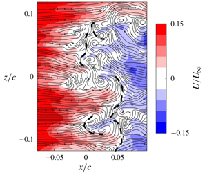
Figure 5. (a) Streamlines obtained from the mean flow in the near-surface ($y=2~\text{mm}$) plane. Colours in the background represent the mean streamwise velocity normalized by free stream speed of the wind tunnel $U_{\infty }$. The positive and negative contours can be identified based on the streamwise direction of the streamlines. (b) Contour lines of the backflow parameter ($\unicode[STIX]{x1D6FE}$) in the near-surface plane, showing intermittency of the separated flow.

The mean velocity field in FOV2 displayed in figure 5(a) is used to gain insight into the near-wall topology in the vicinity of the separation front. The measurement plane is located at $y=2~\text{mm}$, equating to $0.08\unicode[STIX]{x1D6FF}_{99}$ where $\unicode[STIX]{x1D6FF}_{99}$ is the boundary layer thickness at the most upstream position in the FOV ($x/c=-0.15$). The near-wall streamlines obtained in this plane are expected to be similar to the skin-friction lines with minor positional discrepancies according to the investigation of Depardon et al. (Reference Depardon, Lasserre, Boueilh, Brizzi and Borée2005). They studied separated flow around a cube and observed topological consistency when the measurement plane is underneath the location of the main streamwise and spanwise vortical structures. For wall-normal vortices, the near-wall PIV measurements are not expected to deviate from the skin-friction topology except for minor positional discrepancies. In addition, this measurement plane is beneath the zone of maximum turbulence production. As was shown in figure 3, the zone of maximum Reynolds shear stress varies from $y/\unicode[STIX]{x1D6FF}_{99}=0.5$ to 1.5 with increasing streamwise distance.

3.3 Mean skin-friction lines

The near-surface streamlines superimposed on the contours of streamwise velocity magnitude in figure 5(a) reveal a three-dimensional separation. A saddle point is present near midspan and a pair of counter-rotating foci are located at the sides, forming the stall-cell pattern. Such a stall cell pattern has been traditionally observed for thick airfoils at post-stall condition (Winkelman & Barlow Reference Winkelman and Barlow1980; Broeren & Bragg Reference Broeren and Bragg2001; Manolesos & Voutsinas Reference Manolesos and Voutsinas2014b; Dell’Orso & Amitay Reference Dell’Orso and Amitay2018). However, Manolesos et al. (Reference Manolesos, Papadakis and Voutsinas2014) and Ragni & Ferreira (Reference Ragni and Ferreira2016) reported a stall cell for thick airfoils in the nonlinear pre-stall regime of the lift versus angle of attack curve. The detachment-type separation line, shown in figure 5(a) as a dashed line, rolls into the foci and forms tornado-like vortices. The separation line reveals an undulating pattern across the span. Spanwise motion is present at both spanwise sides of the saddle point immediately upstream of the separation line. This is explained by the tendency of flow to escape in the spanwise direction in the presence of an APG. In figure 5(b), the FOV captured most of the incipient detachment points ($\unicode[STIX]{x1D6FE}=0.99$) in the upstream region with the exception of the midspan region as shown by the contours of $\unicode[STIX]{x1D6FE}$. It is noted that there are no points within the FOV where the flow is downstream ($U>0$) or reversed ($U<0$) at all instances, showcasing the intermittency of the flow and the large spatial influence of the present separation.

Figure 6. Contours of (a) streamwise and (b) spanwise components of Reynolds normal stress, and ($c$) Reynolds shear stress in the $x$–$z$ plane. The near-surface streamlines obtained from the mean flow are superimposed on the contours. The negative contours are shown with solid black outlines.

The distance between the two foci in the present study is approximately $0.17s$ (or $0.21c$). Manolesos & Voutsinas (Reference Manolesos and Voutsinas2014a) reported a minimum stall cell width of $0.25s$ for an airfoil with unspecified camber, an aspect ratio of 1.5, and $Re_{c}$ of $1.5\times 10^{6}$. Stall cell width in their investigation include the distance between the outer edges of the two foci, which means the distance between the two foci would have been less than $0.25s$. They also applied zigzag tape over only 10 % of the span to stabilize the stall cell. Dell’Orso & Amitay (Reference Dell’Orso and Amitay2018) observed a stall cell with an estimated distance of $0.18s$ between the two foci for Reynolds numbers between $Re_{c}=4.0\times 10^{5}$ and $4.5\times 10^{5}$. Their study was conducted on a symmetric NACA 0015 airfoil with an aspect ratio of 4.0 and no trip wire was applied. It is also important to note that the stall cell observed by Dell’Orso & Amitay (Reference Dell’Orso and Amitay2018) was in the post-stall regime while the smallest stall cell of Manolesos & Voutsinas (Reference Manolesos and Voutsinas2014a) was observed for trailing-edge separation in the pre-stall regime. Considering the potential effects of angle of attack, airfoil profile, aspect ratio, type of laminar to turbulent transition, and Reynolds number, the size of the stall cell observed here is comparable to the observations of Manolesos & Voutsinas (Reference Manolesos and Voutsinas2014a) and Dell’Orso & Amitay (Reference Dell’Orso and Amitay2018).

3.4 Reynolds stresses of the near-wall plane

Reynolds stress contours in the near-wall $x$–$z$ plane are presented in figure 6. Once again, the stress terms were normalized by the square of the free stream speed. The contours of $\langle u^{2}\rangle /U_{\infty }^{2}$ and $\langle w^{2}\rangle /U_{\infty }^{2}$ both reveal a symmetric pattern about midspan. By comparing the $\unicode[STIX]{x1D6FE}$ contours in figure 5(b) with the distribution of normal Reynolds stresses, it is evident that the largest $\langle u^{2}\rangle /U_{\infty }^{2}$ and $\langle w^{2}\rangle /U_{\infty }^{2}$ exist just upstream of where the separation line is most likely to be located (i.e. $\unicode[STIX]{x1D6FE}\approx 0.50$). The increased fluctuation of both streamwise and spanwise velocity in this region indicates the large turbulence and intermittency of the flow structures that are present at the separation front. Downstream of the mean separation line, both $\langle u^{2}\rangle /U_{\infty }^{2}$ and $\langle w^{2}\rangle /U_{\infty }^{2}$ begin to decrease as the shear layer detaches from the surface and departs from the $x$–$z$ plane of PIV. This agrees with the stress contours in the streamwise–wall-normal plane (figure 3), which show little mixing in the vicinity of the wall within the recirculation region.

The contours of the Reynolds shear stress shown in figure 6(c) are different from the contours of the normal stresses, as large magnitudes of shear stress appear in streamwise-elongated streaks. The streaks of large $\langle uw\rangle /U_{\infty }^{2}$ near $z/c=\pm 0.03$ are located along the detachment lines emanating from the saddle point of the mean flow. The secondary regions of large $\langle uw\rangle$ at $z/c=\pm 0.08$ are located at the same spanwise position as the two counter-rotating foci. There is also a deficit region of $\langle uw\rangle /U_{\infty }^{2}$, which is also elongated in the streamwise direction, and overlaps with the undulating part of the separation line at $z/c=\pm 0.05$.

4.1 Energy spectra

A discrete Fourier transform (DFT) was performed on the fluctuating velocity components obtained from the time-resolved images in FOV2 to identify the energy spectrum of the frequencies present in the flow. Welch’s method was used to reduce spectral variance by performing DFT over overlapping segments and then averaging the results (Heinzel, Rüdiger & Schilling Reference Heinzel, Rüdiger and Schilling2002). Hanning windows with 50 % overlap were applied to the segments to achieve amplitude flatness among all data points (Heinzel et al. Reference Heinzel, Rüdiger and Schilling2002). A segment length of 0.50 s (874 images) was used, resulting in a frequency resolution of 2.0 Hz. The spectral density was evaluated for each set of time-resolved data (2.86 s) and then averaged (five sets in total).

The power spectral density (PSD) of the fluctuating streamwise velocity is presented in figure 7(a) and the PSD of the fluctuating spanwise velocity is shown in figure 7(b). Three points of interest along the midspan ($z=0$) were selected: one upstream of the mean separation ($x/c=-0.05$), one at the saddle point ($x/c=0$) and another within the region of reverse flow ($x/c=0.05$). The three points were selected to determine the change of the frequency spectrum with increasing probability of backflow (i.e. decreasing $\unicode[STIX]{x1D6FE}$). Spectral analysis of the fluctuating velocities at locations away from midspan were also investigated and yielded similar results.

Figure 7. Power spectral density of the fluctuating (a) streamwise and (b) spanwise velocity at a location upstream of the mean separation point ($x/c=-0.05$), at the saddle point ($x/c=0$), and a point in the backflow region ($x/c=0.05$) along midspan ($z=0$).

As is evident in the plots of figure 7, the low-frequency fluctuations have a large kinetic energy at all three points. The energy of the velocity fluctuations decreases sharply with increasing frequency. No strong local peak is observed in the PSDs, indicating the absence of a strong periodic shedding process. At the low frequency range, the streamwise PSDs show a similar energy for all three points. However, at higher frequencies, the energy reduces with streamwise distance. Since the backflow parameter also decreases with streamwise distance, the reduced high-frequency energy coincides with a larger probability of backflow motions.

Considering spanwise velocity fluctuations in figure 7(b), the low-frequency energy is smaller at the upstream point than it is at mean separation and within the backflow region. Investigation of the data at spanwise locations of $z/c=\pm 0.05$ and $\pm 0.10$ also revealed smaller energy of low-frequency content at locations upstream of the mean separation line. The PSD at $z/c=\pm 0.05$ and $\pm 0.10$ are excluded for brevity. At higher frequencies, the energy at the upstream points is larger. This trend indicates the presence of strong low-frequency spanwise motions at the separation point and its downstream locations (i.e. regions where $\unicode[STIX]{x1D6FE}\leqslant 0.50$) as the flow turns in the spanwise direction in response to the APG. The presence of the spanwise motions was evident in the mean flow of figure 5(a) and $\langle w^{2}\rangle$ contours of figure 6(c).

Zaman et al. (Reference Zaman, Mckinzie and Rumsey1989) conducted a study on the oscillation of flow around a stalled airfoil and concluded that bluff body vortex shedding appeared during deep stall at high angles of attack with a Strouhal number of 0.2. The Strouhal number was evaluated by normalizing the frequency, $f$, by the projected height of the airfoil and the free stream speed ($St=fc\sin \unicode[STIX]{x1D6FC}/U_{\infty }$). At lower angle of attack, the vortex shedding frequency was replaced with a Strouhal number in the range of 0.02–0.05, which was associated with a shallow stall due to trailing-edge separation. A similar low-frequency phenomenon was observed by Yon & Katz (Reference Yon and Katz1998) for stalled airfoils that showed stall cell pattern. Zaman et al. (Reference Zaman, Mckinzie and Rumsey1989) attributed this low-frequency fluctuation to the transition of flow between a stalled and unstalled state. The second horizontal axis of figure 7 shows $St$, estimated using $fc\sin \unicode[STIX]{x1D6FC}/U_{\infty }$. Most frequency content contained within the flow appears to be less than the bluff body shedding frequency of $St=0.20$. This agrees with the intermittency of trailing-edge separation as it is constantly alternating between forward and reverse flow, i.e. separated and attached.

4.2 Spatial organization of critical points

A sample snapshot of the instantaneous skin-friction lines is presented in figure 8(a) along with background contours of the normalized instantaneous streamwise velocity ($U/U_{\infty }$). This figure provides a glimpse of the complicated nature of the flow field under investigation. The relatively parallel skin-friction at the upstream boarder of the FOV becomes chaotic as the flow evolves from an attached boundary layer to a separated flow with patches of backflow. The instantaneous separation line is not well defined in the visualization. Saddle points, foci and nodes can be observed throughout. These structures are intertwined with each other and the small-scale turbulence, making it hard to isolate individual structures. There is also no distinct resemblance of a stall cell in this instantaneous visualization. In figure 8(b), background contours of two-dimensional $Q$-criterion (Jeong & Hussain Reference Jeong and Hussain1995) are used to show vortices with strong local rotation within the FOV. Although several patches of large $Q$ are observed, no distinct pair of counter-rotating vortices is observed to guide us toward identifying a stall cell pattern.

Figure 8. Snapshot of the instantaneous near-surface streamlines with a background contour of (a) normalized streamwise velocity and (b) two-dimensional $Q$-criterion. The sign of the contours in (a) can be identified using the streamwise direction of the streamlines.

Figure 9. Filtered streamlines of the instantaneous velocity field in figure 8 with (a) instantaneous streamwise velocity and (b) two-dimensional $Q$-criterion shown in the background. A moving average filter with cutoff frequency at $St=0.05$ was applied. Once again, the colour of the contours in (a) can be identified through the streamwise direction of the streamlines. Rectangles 1 and 3 in (b) show backward stall cells, while rectangle 2 shows a forward stall cell.

In order to remove the small-scale, high-frequency structures from the instantaneous snapshots, a moving average filter is applied to the time-resolved data. The filter is used to isolate the low-frequency motion shown in the spectral analysis of figure 7 and observed in past studies (Zaman et al. Reference Zaman, Mckinzie and Rumsey1989; Yon & Katz Reference Yon and Katz1998). The moving average filter acts as a low-pass filter with a $-3~\text{dB}$ cutoff frequency at $St=0.05$, which was chosen based on the values provided by Zaman et al. (Reference Zaman, Mckinzie and Rumsey1989). They stated that the low frequency motions associated with a mild stall have a non-dimensional frequency between $St=0.02$ and 0.05. Yon & Katz (Reference Yon and Katz1998) later connected this low frequency motion to airfoils with stall cell pattern. This cutoff frequency corresponds to a kernel size of $k=200$ snapshots for the image acquisition frequency of 1750 Hz, which spans over 0.114 s. The instantaneous snapshot of figure 8 has been filtered as described above and is shown in figure 9(a) with normalized instantaneous velocity and in figure 9(b) with $Q$-criterion in the background.

At a first glance of the skin-friction lines in figure 9, it is observed that the majority of the small turbulent vortices with a shorter life-time have been removed from the snapshot due to filtering. The separation structures also appear to be more identifiable through visual inspection. The separation front is three-dimensional and made up of many local separation lines forming from small-scale saddle points. A few of these local separation lines are shown by the dashed lines in figure 9(a). All these separation lines pass through a saddle point and the neighbouring skin-friction lines converge as they approach the separation line. However, even after application of the filter, there is no distinct separation line that extends across the entire spanwise length of the FOV as seen in the mean flow of figure 5(a).

According to Surana, Grunberg & Haller (Reference Surana, Grunberg and Haller2006), the separation line emanating from a saddle point must terminate at either a node or focus, which is true for the instantaneous skin-friction lines shown in figure 9. The local separation lines sometimes terminate in a pair of counter-rotating foci as identified by the three rectangular boxes in figure 9(b), resulting in ‘instantaneous stall cells’ that are smaller than the stall cell in the mean skin-friction pattern. It is also possible for two separation lines to terminate at the same focus as highlighted by the overlap of the instantaneous stall cells identified by boxes 2 and 3 in figure 9(b). By inspecting the visualizations, the width of these instantaneous stall cells (i.e. distance between the two foci) can range from $0.02s$ to $0.06s$ ($0.02c$–$0.07c$), which is an order of magnitude smaller than the width of the mean stall cell.

Table 2. Advection velocities and speed of saddle points and foci evaluated based on the tracks detected in five sets of filtered time-resolved data.

Further inspection of figure 9 shows two types of stall cell in this instantaneous visualization based on the flow direction between the foci pair and the relative location of the saddle point. There are local stall cells with a strong backward flow motion such as the ones identified in rectangles 1 and 3. The saddle point of these stall cells is pushed to the upstream side of the foci pair. The second type of stall cell consists of a strong inrush of forward flow as shown in rectangle 2. As a result, the saddle point is observed on the downstream side of the foci. Based on the direction of the flow between the foci pair, these two structures will be referred to as backward and forward stall cells, respectively.

Figure 10. (a) Visualization of the detected tracks of saddle points, clockwise foci, and counter-clockwise foci over 1.0 s. Saddle points, clockwise foci, and counter-clockwise foci are shown with black, medium grey (green) and light grey (yellow) tracks, respectively. Tracks shown in the figures have a minimum length of 25 frames (0.014 s). The lower two plots show projections of the locations of the (b) saddle points and (c) foci obtained from 2.5 s of time-resolved data onto the $x$–$z$ plane.

The above analysis was repeated using a low-pass filter with different cutoff frequencies, which varied from $St=0.02$ to 0.2. In general, the number of critical points increased with increasing cutoff frequency due to the appearance of a larger number of small-scale structures. At the highest cutoff frequency of $St=0.2$, the organization of instantaneous stall cells became intertwined with small-scale structures, thus making the instantaneous structures less apparent. For the lowest cutoff of $St=0.02$, it appeared that the instantaneous stall cells were partially filtered. However, the small instantaneous stall cells were present in all cases.

The low-pass filtered velocity fields from FOV2 have also been used to detect the critical points and track them in time using the algorithm described in § 2.4. A visualization of the trajectories of saddle points, clockwise (CW) foci, and counter-clockwise (CCW) foci based on 1.0 s of time-resolved data are shown in figure 10(a). The left-side axes of the plot show the $x$ and $z$ coordinates of the critical points while the horizontal axis shows time. The figure indicates that the translations of the critical points in the $x$ and $z$ directions are small since most of the tracks appear as relatively straight lines. The average streamwise advection velocity, $\langle U_{a}\rangle$, and the average streamwise advection speed, $\langle |U_{a}|\rangle$, for saddle points and foci were calculated from the detected tracks and are shown in table 2. The same calculation is also carried out for the average spanwise advection velocity, $\langle W_{a}\rangle$, and its speed, $\langle |W_{a}|\rangle$. Here, the absolute operator, $|\,\ldots \,|$, is applied to isolate the effect of the direction. All five sets of filtered time-resolved datasets were considered to obtain the values shown in table 2. Statistical convergence of the advection velocities was verified by plotting the parameter against the number of sample points used for its calculation. The convergence tests showed that the values have statistically converged to their mean values. The random error of the values presented in table 2 were determined by finding the difference between the maximum and minimum value (the range) for the trailing 20 % of the convergence curve.

Advection of the saddle and focus points is observed in both the streamwise and spanwise directions as they both possess finite $\langle |U_{a}|\rangle$ and $\langle |W_{a}|\rangle$ values. The sign of $\langle U_{a}\rangle$ is positive for saddle and focus points, revealing that, on average, these structures tend to move in the downstream direction. However, the larger value of $\langle |U_{a}|\rangle$ with respect to $\langle U_{a}\rangle$ indicates that there is also a significant amount of backward advection in the upstream direction. Since saddle points and foci form along the separation lines of the instantaneous stall cells, the advection of these critical points is associated with movement and intermittency of the separation lines. Consequently, the separation lines are also expected to move in both the upstream and downstream directions with a slight tendency towards the downstream direction. The spanwise advection speed of the structures is also comparable with their streamwise speed. However, there is no spanwise preference as the average spanwise advection, $\langle W_{a}\rangle$, is negligible.

The tracks of saddle points and foci have been projected onto the $x$–$z$ plane and presented in figures 10(b) and 10(c), respectively. These figures visualize the motion of the critical points in the $x$–$z$ plane and approximate their probability density distributions. In both figures, the locations of the critical points form a V-shape distribution, similar to the pattern of the mean stall cell. The saddle points in figure 10(b) are evenly distributed between both halves of the span. In figure 10(c), the tracks of clockwise foci are shown in dark grey (green) while the tracks of counter-clockwise foci are shown in light grey (yellow). It is evident that the counter-clockwise foci are localized at the bottom of the FOV, while foci with clockwise rotation are centralized at the top. This preferential concentration of the foci structures is believed to form the foci pair of the mean stall cell pattern that was observed in figure 5(a), i.e. the average of counter-clockwise foci located at the bottom of the FOV forms the large mean counter-clockwise focus in the mean-velocity field, and vice versa for the clockwise focus that appears at the top of the FOV.

Figure 11. The formation and dissipation of (a–d) a forward stall cell and (e–h) a backward stall cell due to local concentrations of strong streamwise momentum. The colours in the background correspond to the normalized streamwise velocity. Videos of the process are provided in movies 2 and 3 of the supplementary materials online.

4.3 Instantaneous forward and backward stall cells

Inspection of the time-resolved skin-friction lines in movie 1 of the supplementary material available at https://doi.org/10.1017/jfm.2020.106 shows that foci pairs tend to form near regions of strong local flow at the separation front. This local flow results in high shear and the formation of counter-rotating, tornado-like vortices (the foci pair). In one presently observed scenario, the strong local flow originates from an influx of streamwise momentum from upstream flow in the form of a single high-speed streak. The high-momentum flow pierces an already existing separation front and forms the foci pair. The resultant skin-friction pattern is a saddle point with a pair of counter-rotating foci, i.e. an instantaneous stall cell. The motion corresponding to this topology is separation via a pair of tornado-like vortices (Délery Reference Délery2013). As shown in the visualization of figure 9, these instantaneous stall cells can exist with either forward or backward orientations. In contrast to the above description, the latter forms as a result of a strong backflow from the downstream side of the separation front. By identifying the instantaneous stall cells as a pair of tornado-like vortices (Délery Reference Délery2013), it is hypothesized that streamwise momentum is converted into wall-normal momentum during the formation of these structures.

The instantaneous stall cell formation described above is visualized in figure 11. Figure 11(a–d) show the formation of a forward stall cell due to a strong downstream flow, while figure 11(e,f) show the formation of a backward stall cell due to a strong backflow. The process is demonstrated through carefully selected timestamps here, but videos of the processes are provided in movies 2 and 3 of the supplementary material. Once again, these streamlines were obtained from the filtered data described in § 4.2. The subfigures contain a zoomed-in view of the structures with normalized instantaneous streamwise velocity ($U/U_{\infty }$) plotted in the background of the streamlines. The separation lines of nearby saddle points are represented by dashed lines to highlight the movement of the instantaneous separation line.

Figure 11(a) reveals the skin-friction lines before the influx of streamwise momentum. The dashed lines in the subfigure are clearly separation lines because neighbouring skin-friction lines converge towards it. The local separation line on the left comes from a saddle point that is outside of the cropped FOV. After 0.055 s, a pair of foci is formed due to an inrush of strong streamwise flow as indicated by the arrow in figure 11(b). The centres of the two foci are located at approximately $(x/c,z/c)=(0,0)$ and (0.01, $-0.03$) in the figure. The two foci indicate that the local flow ejects from the surface via a pair of tornado-like vortices that contain both spanwise and wall-normal momentum. As the incoming momentum subsides (figure 11c), the pair of foci eventually disintegrates and smaller, unstable structures are left behind as shown in figure 11(d). The formation process of a backward stall cell is the same but is spatially reversed as can be seen in figure 11(e–h). The strong backflow seen in figure 11(f) results in a pair of foci located at $(x/c,z/c)=(0,0.01)$ and (0.01, $-0.03$).

4.4 High-speed streaks

In § 4.3, it was evident that foci are located at high-shear regions of forward or backward flow at the separation front. One possible scenario is that these high-shear regions are created by an inrush of streamwise momentum from upstream high-speed streaks of the turbulent boundary layer. If this is the case, then the width of instantaneous stall cells should be similar to the spanwise spacing between high-speed streaks. In this section, the spanwise distance between adjacent high-speed streaks ($\unicode[STIX]{x1D706}_{z}$) in the upstream turbulent boundary layer is evaluated through spatial autocorrelation of the streamwise fluctuating velocity in the spanwise direction, which is then compared with the size of instantaneous stall cells determined previously. The normalized correlation coefficient, which is determined using

(4.1)$$\begin{eqnarray}\unicode[STIX]{x1D70C}(\unicode[STIX]{x0394}z)=\frac{\langle u(x_{i},z,t_{n})\cdot u(x_{i},z+\unicode[STIX]{x0394}z,t_{n})\rangle }{u_{\mathit{rms}}(x_{i},z,t_{n})^{2}},\end{eqnarray}$$

can be a value between $-1$ and $+1$. The correlation curve is calculated for the $n$th snapshot at a specified streamwise position $x_{i}$. At zero shift ($\unicode[STIX]{x0394}z=0$), the signal aligns perfectly and return a value of $\unicode[STIX]{x1D70C}=1$. As the signal is shifted, the correlation coefficient decreases until a local minimum value is reached. At this minimum, the signal has been shifted by half the spanwise wavelength of the streamwise fluctuations and can therefore be used to determine the associated wavelength. The autocorrelation function was applied to the cyclic data set for faster statistical convergence. Histograms of the spanwise wavelengths have been generated and a log-normal distribution was used to model the probability density function (p.d.f.) of the results.

The p.d.f.s of the spanwise wavelengths are plotted for three different chordwise positions in figure 12 to investigate the effect of chordwise position on streak width. The spanwise wavelengths of the streaks presented here are normalized by the span. The chordwise positions chosen correspond to an upstream location ($x/c=-0.05$), the mean separation point ($x/c=0$) and a downstream location ($x/c=0.05$). All three distributions are unimodal and are right-skewed to varying degrees. The upstream ($x/c=-0.05$) distribution features a peak located at $\unicode[STIX]{x1D706}_{z}/s=0.030$. In § 4.2, it was found that the width of instantaneous stall cells can range from approximately $0.02s$–$0.06s$. The p.d.f. corresponding to $x/c=-0.05$ reveals that a large majority of the upstream streak widths fall within this range. Consequently, the size of the instantaneous stall cells likely scales with the spacing between upstream high-speed streaks.

As the flow progresses downstream, the peak of the distribution moves to the right while the distribution broadens. At $x/c=0$ and 0.05, the peak is shifted to $\unicode[STIX]{x1D706}_{z}/s=0.034$ and 0.044, respectively. Both of these peak locations (i.e. the most probable values) also fall within the aforementioned range of instantaneous stall cell sizes. The p.d.f. at the downstream location ($x/c=0.05$) is quite broad, indicating that the size of the streaks varies considerably post separation. This is quantified by the standard deviation of the distribution, which increases from 0.011 to 0.022 between $x/c=-0.05$ and 0.05. The change in the p.d.f.s reinforces the notion that streaks evolve into two foci and a saddle structure at separation. As the streaks vanish from the measurement plane, the spacing between the streaks increases and $\unicode[STIX]{x1D706}_{z}$ will tend towards a larger value.

The evolution of the high-speed streaks moving through the measurement plane is shown using three-dimensional isosurfaces in figure 13(a). These isosurfaces have also been projected onto the $x$–$t$ axis in figure 13(b) to highlight the advection of streaks in the streamwise direction. The streaks shown in the figure correspond to a segment of the unfiltered time-resolved data. There are a large number of high-speed streaks in the upstream region ($x/c<0$) and a significant number of the streaks subside before they reach the downstream section of the FOV. This agrees with the p.d.f.s in figure 12 and further supports the notion that streamwise momentum from high-speed streaks forms separation structures once they reach the separation front instead of persisting downstream.

Figure 12. Probability density functions of the spanwise wavelength of high-speed streaks ($\unicode[STIX]{x1D706}_{z}/s$) at three different chordwise positions. The wavelengths were determined by spatial autocorrelation of the fluctuating streamwise velocity using (4.1) and were fitted with a log-normal distribution.

Figure 13. (a) Isosurfaces of the fluctuating streamwise velocity corresponding to $u/U_{\infty }=0.12$. (b) The isosurfaces projected onto the $x$–$t$ axis to highlight the advection velocity of streaks in the streamwise direction.