


1 Introduction
The theory of scattering of long waves by small bodies has a long history that can be traced back to Lord Rayleigh (Strutt Reference Strutt1897) in his treatment of aerial and electric waves. The formal procedure of matched asymptotics has been applied in many areas of wave propagation and extended to higher orders, subjected to either Dirichlet or Neumann boundary conditions. Extensive reviews can be found in the articles by Crighton & Leppington (Reference Crighton and Leppington1973), Martin & Dalrymple (Reference Martin and Dalrymple1988), Kleinman & Vainberg (Reference Kleinman and Vainberg1994) and Guo & McIver (Reference Guo and McIver2011) and in the books by Varadan & Varadan (Reference Varadan and Varadan1968) and Martin (Reference Martin2006), mostly for sound waves in solids and fluids in a non-rotating system.
Affected by the Earth’s rotation, tidal diffraction by large coastline features has been reviewed comprehensively by LeBlond & Mysak (Reference LeBlond and Mysak1987). Other relevant works include Crease (Reference Crease1956) for a semi-infinite barrier, Buchwald (Reference Buchwald1971) for a cornered coast, Buchwald & Miles (Reference Buchwald and Miles1974) for a gap in a long barrier, Pinsent (Reference Pinsent1971) for a depth discontinuity, Pinsent (Reference Pinsent1972) for small irregularities along a straight coast, and Howe & Mysak (Reference Howe and Mysak1973) for a randomly irregular coastline, etc. However, for tides around islands of finite size, analytical theories are relatively scarce. Proudman (Reference Proudman1915) obtained the exact solution for a circular island and treated a small elliptical cape and its limit of a thin barrier protruding from a coast, but confined his analysis to the near field by employing the potential theory approximation. Refraction and diffraction of Rossby waves by a long step and a ridge near slowly varying one-dimensional bathymetry were first analysed by Rhines (Reference Rhines1969a). Two-dimensional diffraction by islands and seamounts of circular geometries was also covered by Rhines (Reference Rhines1969b).
While tidal diffraction excluding the  $\unicode[STIX]{x1D6FD}$ effect is governed by the familiar Helmholtz equation, the oblique derivative boundary condition due to the Coriolis parameter
  $f$,
$f$,
 $$\begin{eqnarray}\frac{\unicode[STIX]{x2202}\unicode[STIX]{x1D701}}{\unicode[STIX]{x2202}n}-\text{i}\frac{f}{\unicode[STIX]{x1D714}}\frac{\unicode[STIX]{x2202}\unicode[STIX]{x1D701}}{\unicode[STIX]{x2202}s}=0,\end{eqnarray}$$
is of neither Dirichlet nor Neumann form. Analytical theories for finite scatterers of general size and geometry are known to be difficult (Krutitskii Reference Krutitskii2001). Explicit numerical computations based on integral equations for an island in a sea of constant depth have been reported by Abel-Hafz, Essawy & Moubark (Reference Abel-Hafz, Essawy and Moubark1997), who imposed the Neumann boundary condition on the coast instead of (1.1). Al-Hawaj, Essawy & Faltas (Reference Al-Hawaj, Essawy and Faltas1991) computed tidal impact on coastal irregularities by ignoring the Earth’s rotation in the approximate Green’s function. Hence the effect of the Earth’s rotation was not properly accounted for by these authors. Similar extensions have been made by Essawy (Reference Essawy1984, Reference Essawy1995). Theoretical treatments based on integral equations aiming at numerical solution for an island of any size have been advanced by Krutitskii (Reference Krutitskii2001) and Martin (Reference Martin2001). Both papers focus on the mathematical foundations without executing explicit computations. Hence quantitative results for physical applications are thus not yet available.
The present work is motivated by recent proposals to construct artificial coastal barriers for harnessing tidal power. Unlike existing schemes based either on using a strong tidal current or building barrages to produce a higher water level in a one- or two-basin reservoir (Baker Reference Baker2000), the dynamic tidal power (DTP) system initiated by Hulsbergen et al. (Reference Hulsbergen, Steijn, Hassan, Klopman and Hurdle2005) aims at tides of low or moderate amplitudes, by using an artificially constructed barrier approximately 50 km in length. Several computational models are available for estimating the practical potential. Since the barrier length is much smaller than the typical tidal wavelength, an analytical prediction by matched asymptotics is convenient for the idealized geometry despite the boundary condition (1.1). Here we describe a leading-order theory for tidal diffraction by a small island or cape, and use the predicted coastal runup for the limiting case of a coastal barrier to give a convenient estimate of the available power. We also work out the scattering amplitude in the far field, which may be of interest for environmental considerations.
2 Governing equations of long waves in a rotating sea
We consider a tidal wave of single frequency  $\unicode[STIX]{x1D714}$. In a rotating sea of constant depth
  $h$, the conservation equations for mass,
 $$\begin{eqnarray}\text{i}\unicode[STIX]{x1D714}\unicode[STIX]{x1D701}+h(u_{x}+v_{y})=0,\end{eqnarray}$$
and momentum,
 $$\begin{eqnarray}\text{i}\unicode[STIX]{x1D714}u-fv=-g\unicode[STIX]{x1D701}_{x},\quad \text{i}\unicode[STIX]{x1D714}v+fu=-g\unicode[STIX]{x1D701}_{y},\end{eqnarray}$$
 are well known (Proudman Reference Proudman1953), where  $f$ is the Coriolis parameter. The time factor
  $\text{e}^{\text{i}\unicode[STIX]{x1D714}t}$ is assumed but omitted for brevity and is implied from now on.
Equations (2.2) can be solved for the velocity components:
 $$\begin{eqnarray}k^{2}hu=\text{i}\unicode[STIX]{x1D714}\unicode[STIX]{x1D701}_{x}+f\unicode[STIX]{x1D701}_{y},\quad k^{2}hv=-f\unicode[STIX]{x1D701}_{x}+\text{i}\unicode[STIX]{x1D714}\unicode[STIX]{x1D701}_{y},\end{eqnarray}$$
where
 $$\begin{eqnarray}k^{2}=\frac{\unicode[STIX]{x1D714}^{2}-f^{2}}{C^{2}},\quad C=\sqrt{gh}.\end{eqnarray}$$
 Substituting (2.3) in (2.1),  $\unicode[STIX]{x1D701}$ satisfies the familiar Helmholtz equation:
 $$\begin{eqnarray}\unicode[STIX]{x1D701}_{xx}+\unicode[STIX]{x1D701}_{yy}+k^{2}\unicode[STIX]{x1D701}=0.\end{eqnarray}$$
 We shall limit this study to the northern hemisphere and diurnal tides, so that  $f>0$,
  $\unicode[STIX]{x1D714}>f$ and
  $k^{2}>0$.
3 Elliptic island in open sea
For an elliptic island in the open sea, the full solution for all island sizes can be derived, in principle, by using Mathieu functions (as in Stamnes & Spjelkavik (Reference Stamnes and Spjelkavik1995) for classical waves). The task would require elaborate algebra and computations, and is not known to have been carried out. We shall apply the technique of matched asymptotics to derive the approximate solution for a small island. In particular, we aim to find the scattered waves in the far field to complement Proudman’s solution in the near field.
3.1 Outer solution: incident and scattered tides
Let us define the outer solution  $\unicode[STIX]{x1D701}$ valid in the region
  $kr\geqslant O(1)$ to be the sum of the incident tide
  $\unicode[STIX]{x1D701}^{I}$ and the scattered tide
  $\unicode[STIX]{x1D701}^{S}$,
 $$\begin{eqnarray}\unicode[STIX]{x1D701}=\unicode[STIX]{x1D701}^{I}+\unicode[STIX]{x1D701}^{S},\end{eqnarray}$$
 where  $\unicode[STIX]{x1D701}^{I}$ is assumed to be a simple Poincaré wave incident at angle
  $\unicode[STIX]{x1D703}_{i}$,
 $$\begin{eqnarray}\unicode[STIX]{x1D701}^{I}=A\text{e}^{-\text{i}\boldsymbol{k}\boldsymbol{\cdot }\boldsymbol{x}}=A\text{e}^{\text{i}(\unicode[STIX]{x1D6FC}x+\unicode[STIX]{x1D6FD}y)}=A\text{e}^{-\text{i}kr\cos (\unicode[STIX]{x1D703}-\unicode[STIX]{x1D703}_{i})},\end{eqnarray}$$
 with  $(x,y)=r(\cos \unicode[STIX]{x1D703},\sin \unicode[STIX]{x1D703})$ and
  $(\unicode[STIX]{x1D6FC},\unicode[STIX]{x1D6FD})=-k(\cos \unicode[STIX]{x1D703}_{i},\sin \unicode[STIX]{x1D703}_{i})$. For
  $\unicode[STIX]{x1D6FC},\unicode[STIX]{x1D6FD}>0$,
  $\unicode[STIX]{x03C0}<\unicode[STIX]{x1D703}_{i}<3\unicode[STIX]{x03C0}/2$. Such waves are possible only if
  $\unicode[STIX]{x1D714}/f>1$.
Using (2.3), the velocity components of the incident tide are
 $$\begin{eqnarray}u^{I}=gA\frac{-\unicode[STIX]{x1D714}\unicode[STIX]{x1D6FC}+\text{i}f\unicode[STIX]{x1D6FD}}{\unicode[STIX]{x1D714}^{2}-f^{2}}\text{e}^{\text{i}(\unicode[STIX]{x1D6FC}x+\unicode[STIX]{x1D6FD}y)},\quad v^{I}=gA\frac{-\unicode[STIX]{x1D714}\unicode[STIX]{x1D6FD}-\text{i}f\unicode[STIX]{x1D6FC}}{\unicode[STIX]{x1D714}^{2}-f^{2}}\text{e}^{\text{i}(\unicode[STIX]{x1D6FC}x+\unicode[STIX]{x1D6FD}y)}.\end{eqnarray}$$
 Suggested by the classical theory of sound around a circular cylinder, the scattered tide  $\unicode[STIX]{x1D701}^{S}$ can be constructed by a series of poles of ascending order:
 $$\begin{eqnarray}\unicode[STIX]{x1D701}^{S}=C_{0}\text{H}_{0}(kr)+\mathop{\sum }_{m=1}^{\infty }[C_{m}\cos m\unicode[STIX]{x1D703}+S_{m}\sin m\unicode[STIX]{x1D703}]\text{H}_{m}(kr).\end{eqnarray}$$
 Throughout this work  $\text{H}_{m}(kr)$ stands for Hankel functions
  $\text{H}_{m}^{(2)}(kr)$ for brevity. For general island geometries in a rotating sea, the strengths
  $C_{m},S_{m},m=0,1,2,\ldots ,$ are as yet unknown. For small bodies with size of
  $O(a)$, the series is expected to be dominated by poles of the first two orders with strengths proportional to
  $O(k^{2}a^{2})$, i.e.
 $$\begin{eqnarray}\unicode[STIX]{x1D701}^{S}\approx \unicode[STIX]{x1D701}_{0}^{S}+\unicode[STIX]{x1D701}_{1}^{S},\quad \text{where }\unicode[STIX]{x1D701}_{0}^{S}=C_{0}\text{H}_{0},\unicode[STIX]{x1D701}_{1}^{S}=\left(C_{1}\cos \unicode[STIX]{x1D703}+S_{1}\sin \unicode[STIX]{x1D703}\right)\text{H}_{1}(kr).\end{eqnarray}$$
 For later asymptotic matching with the inner solution near the small island  $r\leqslant O(a)$, we approximate the incident tide for small
  $kr$ by
 $$\begin{eqnarray}\frac{\unicode[STIX]{x1D701}_{in}^{I}}{A}\approx 1+\text{i}\unicode[STIX]{x1D6FC}x+\text{i}\unicode[STIX]{x1D6FD}y-\frac{1}{2}(\unicode[STIX]{x1D6FC}^{2}x^{2}+\unicode[STIX]{x1D6FD}^{2}y^{2})-\unicode[STIX]{x1D6FC}\unicode[STIX]{x1D6FD}xy+O(k^{3}a^{3}).\end{eqnarray}$$
The linear part above corresponds to the irrotational current near the island:
 $$\begin{eqnarray}u_{in}^{I}\equiv u^{I}(0,0)=gA\frac{-\unicode[STIX]{x1D714}\unicode[STIX]{x1D6FC}+\text{i}f\unicode[STIX]{x1D6FD}}{\unicode[STIX]{x1D714}^{2}-f^{2}},\quad v_{in}^{I}\equiv v^{I}(0,0)=gA\frac{-\unicode[STIX]{x1D714}\unicode[STIX]{x1D6FD}-\text{i}f\unicode[STIX]{x1D6FC}}{\unicode[STIX]{x1D714}^{2}-f^{2}}.\end{eqnarray}$$
 The quadratic part of (3.6) is rotational with the vorticity of order  $O(k^{2}a^{2})$, and is needed for determining
  $C_{0}$, as stressed by Martin & Dalrymple (Reference Martin and Dalrymple1988) in their matched asymptotic theory of long sound wave scattering by gratings in a non-rotating fluid.
In the far field where  $kx,ky,kr\gg 1$, the scattered tide is asymptotically
 $$\begin{eqnarray}\unicode[STIX]{x1D701}^{S}=\unicode[STIX]{x1D701}_{0}^{S}+\unicode[STIX]{x1D701}_{1}^{S}\approx C_{0}\sqrt{\frac{2}{\unicode[STIX]{x03C0}kr}}\text{e}^{-\text{i}(kr-\unicode[STIX]{x03C0}/4)}+(S_{1}\sin \unicode[STIX]{x1D703}+C_{1}\cos \unicode[STIX]{x1D703})\sqrt{\frac{2}{\unicode[STIX]{x03C0}kr}}\text{e}^{-\text{i}(kr-\unicode[STIX]{x03C0}/4-\unicode[STIX]{x03C0}/2)}.\end{eqnarray}$$
Using the properties of Hankel functions with small argument, the inner approximation of the scattered tide is
 $$\begin{eqnarray}\unicode[STIX]{x1D701}^{S}=\unicode[STIX]{x1D701}_{0,in}^{S}+\unicode[STIX]{x1D701}_{1,in}^{S},\end{eqnarray}$$
where the source part is
 $$\begin{eqnarray}\unicode[STIX]{x1D701}_{0,in}^{S}\approx -C_{0}\frac{2\text{i}}{\unicode[STIX]{x03C0}}\ln \frac{kr}{2}\end{eqnarray}$$
and the doublet part is
 $$\begin{eqnarray}\unicode[STIX]{x1D701}_{1,in}^{S}\approx (S_{1}\sin \unicode[STIX]{x1D703}+C_{1}\cos \unicode[STIX]{x1D703})\frac{2\text{i}}{\unicode[STIX]{x03C0}kr}=(S_{1}y+C_{1}x)\frac{2\text{i}}{\unicode[STIX]{x03C0}kr^{2}}.\end{eqnarray}$$
 Use has been made of the relations  $\cos \unicode[STIX]{x1D703}=x/r$ and
  $\sin \unicode[STIX]{x1D703}=y/r$. To determine the pole strengths (
 $C_{0},C_{1},S_{1}$), we turn to the near-field solution defined in the region
  $O(k^{-1})\gg r=O(a)$.
3.2 The near field (the inner solution  $\unicode[STIX]{x1D702}$)

For later determination of the diffraction field, it is convenient to recount Proudman’s inner solution. As noted by Rayleigh (Strutt Reference Strutt1897), the governing Helmholtz equation can be approximated by the Laplace equation with an error  $O(k^{2}a^{2})$. Hence the inner solution can be found in terms of the complex potential
  $w(z)=\unicode[STIX]{x1D719}+\text{i}\unicode[STIX]{x1D713}$. To ensure clarity, we denote the near-field surface displacement by
  $\unicode[STIX]{x1D702}(x,y)$ instead of
  $\unicode[STIX]{x1D701}(x,y)$. Proudman (Reference Proudman1915) showed first that
 $$\begin{eqnarray}-g\unicode[STIX]{x1D702}=\text{i}\unicode[STIX]{x1D714}\unicode[STIX]{x1D719}+f\unicode[STIX]{x1D713},\end{eqnarray}$$
 which follows by integrating either equation in (2.2) and using Cauchy–Riemann conditions. He then used the classic solution of a current  $(U,V)$ passing an elliptical cylinder (see Milne-Thomson Reference Milne-Thomson1955, p. 159ff.):
 $$\begin{eqnarray}\displaystyle w(z)=\frac{1}{2}\left[(U-\text{i}V)\left(z+\sqrt{z^{2}-c^{2}}\right)+(U+\text{i}V)\frac{(a+b)^{2}}{c^{2}}\left(z-\sqrt{z^{2}-c^{2}}\right)\right],\quad & & \displaystyle\end{eqnarray}$$
 where  $(a,b)$ are respectively the major and minor axes of the ellipse,
 $$\begin{eqnarray}\frac{x^{2}}{a^{2}}+\frac{y^{2}}{b^{2}}=1,\end{eqnarray}$$
 and  $c^{2}=a^{2}-b^{2}$. By using elliptical coordinates, it can be shown that
  $\unicode[STIX]{x1D713}=0$ on the elliptical coast.
For later matching with the far field (outer solution), we seek the outer approximation of  $w(z)$ by letting
  $kr\ll 1$ but
  $z/c\sim z/a\gg 1$. Since
 $$\begin{eqnarray}\sqrt{z^{2}-c^{2}}=z-\frac{c^{2}}{2z}+O\left(\frac{c^{4}}{z^{4}}\right),\end{eqnarray}$$
 the outer approximation of  $w(z)$ is
 $$\begin{eqnarray}\displaystyle w_{out} & {\approx} & \displaystyle [Ux+Vy+\text{i}(-Vx+Uy)]\nonumber\\ \displaystyle & & \displaystyle -\,\frac{c^{2}}{4r^{2}}[Ux-Vy-\text{i}(Vx+Uy)]+\frac{c^{2}}{4r^{2}}\frac{a+b}{a-b}[Ux+Vy+\text{i}(Vx-Uy)].\qquad\end{eqnarray}$$
Separating the real and imaginary parts:
 $$\begin{eqnarray}\displaystyle \unicode[STIX]{x1D719}_{out} & {\approx} & \displaystyle [Ux+Vy]-\frac{c^{2}}{4r^{2}}\left[Ux-Vy-\frac{a+b}{a-b}(Ux+Vy)\right]\nonumber\\ \displaystyle & = & \displaystyle [Ux+Vy]-\frac{a+b}{2r^{2}}[-Ubx-Vay],\end{eqnarray}$$
 $$\begin{eqnarray}\displaystyle \unicode[STIX]{x1D713}_{out} & {\approx} & \displaystyle (-Vx+Uy)+\frac{c^{2}}{4r^{2}}\left[(Vx+Uy)+\frac{a+b}{a-b}(Vx-Uy)\right]\nonumber\\ \displaystyle & = & \displaystyle (-Vx+Uy)+\frac{a+b}{2r^{2}}[Vax-Uby].\end{eqnarray}$$
 The outer approximation of the inner solution  $\unicode[STIX]{x1D702}$ is
 $$\begin{eqnarray}\displaystyle \unicode[STIX]{x1D702}_{out} & {\approx} & \displaystyle -\frac{1}{g}\left(\text{i}\unicode[STIX]{x1D714}\unicode[STIX]{x1D719}_{out}+f\unicode[STIX]{x1D713}_{out}\right)=-\frac{1}{g}\left\{(\text{i}\unicode[STIX]{x1D714}U-f\,V)x+(\text{i}\unicode[STIX]{x1D714}V+fU)y\right\}\nonumber\\ \displaystyle & & \displaystyle -\,\frac{1}{g}\left\{\frac{a+b}{2r^{2}}\left[\left(\text{i}\unicode[STIX]{x1D714}Ub+f\,Va\right)x+\left(\text{i}\unicode[STIX]{x1D714}Va-fUb\right)y\right]\right\}.\end{eqnarray}$$
 By equating the coefficients of  $x$ and
  $y$ in (3.19) and (3.6) we obtain
 $$\begin{eqnarray}U=gA\frac{-\unicode[STIX]{x1D714}\unicode[STIX]{x1D6FC}+\text{i}f\unicode[STIX]{x1D6FD}}{\unicode[STIX]{x1D714}^{2}-f^{2}}=u^{I}(0,0),\quad V=gA\frac{-\unicode[STIX]{x1D714}\unicode[STIX]{x1D6FD}-\text{i}f\unicode[STIX]{x1D6FC}}{\unicode[STIX]{x1D714}^{2}-f^{2}}=v^{I}(0,0),\end{eqnarray}$$
to the leading order, which agrees with (3.7), as expected.
The inner solution  $\unicode[STIX]{x1D702}$ represented by (3.13) is therefore completely known from the leading-order terms of the far field, and agrees with Proudman (Reference Proudman1915). This result will be used to find the strength of the doublet
  $C_{1}$ and
  $S_{1}$ in (3.5) in the outer solution
  $\unicode[STIX]{x1D701}_{1}^{S}$.
3.3 Coefficients in the outer solution
By matching the outer approximation of the inner solution ( $\unicode[STIX]{x1D702}_{out}^{I}$, (3.19)) and the inner approximation of the outer solution (
 $\unicode[STIX]{x1D701}_{in,1}^{S}$, (3.11)), we equate the coefficients of
  $x/r^{2}$ and
  $y/r^{2}$, and get, respectively,
 $$\begin{eqnarray}C_{1}=\frac{\text{i}\unicode[STIX]{x03C0}k(a+b)}{4g}(\text{i}\unicode[STIX]{x1D714}Ub+f\,Va)\end{eqnarray}$$
and
 $$\begin{eqnarray}S_{1}=\frac{\text{i}\unicode[STIX]{x03C0}k(a+b)}{4g}(\text{i}\unicode[STIX]{x1D714}Va-fUb).\end{eqnarray}$$
Making use of (3.20), we find the doublet strength,
 $$\begin{eqnarray}C_{1}=\frac{\text{i}\unicode[STIX]{x03C0}k(a+b)}{4g}[-\text{i}\unicode[STIX]{x1D6FC}(\unicode[STIX]{x1D714}^{2}b+f^{2}a)-\unicode[STIX]{x1D714}f\unicode[STIX]{x1D6FD}(a+b)]\frac{gA}{\unicode[STIX]{x1D714}^{2}-f^{2}}\end{eqnarray}$$
and
 $$\begin{eqnarray}S_{1}=\frac{\text{i}\unicode[STIX]{x03C0}k(a+b)}{4g}[-\text{i}\unicode[STIX]{x1D6FD}(\unicode[STIX]{x1D714}^{2}a+f^{2}b)+\unicode[STIX]{x1D714}f\unicode[STIX]{x1D6FC}(a+b)]\frac{gA}{\unicode[STIX]{x1D714}^{2}-f^{2}}.\end{eqnarray}$$
 With these results, the doublet part  $\unicode[STIX]{x1D701}_{1}^{S}$ is now complete. Note that
  $U$ and
  $V$ hence
  $C_{1}$ and
  $S_{1}$ are fixed by the linear terms in (3.6).
In the limiting case of a thin barrier,  $b=0$, and a northward tide,
  $\unicode[STIX]{x1D6FC}=0,~\unicode[STIX]{x1D6FD}=k$, we get
 $$\begin{eqnarray}C_{1}=\frac{\text{i}\unicode[STIX]{x03C0}ka}{4g}(-f\,Va)=\frac{\text{i}\unicode[STIX]{x03C0}k^{2}a^{2}}{4}\frac{\unicode[STIX]{x1D714}f}{\unicode[STIX]{x1D714}^{2}-f^{2}}A\end{eqnarray}$$
and
 $$\begin{eqnarray}S_{1}=\frac{\text{i}\unicode[STIX]{x03C0}k(a)}{4g}(-\text{i}\unicode[STIX]{x1D714}Va)=\frac{\unicode[STIX]{x03C0}k^{2}a^{2}}{4}\frac{\unicode[STIX]{x1D714}^{2}}{\unicode[STIX]{x1D714}^{2}-f^{2}}A,\end{eqnarray}$$
which agrees with Proudman (Reference Proudman1915).
As another limiting case, the doublet coefficients for a circular island in a northward incident tide,  $\unicode[STIX]{x1D6FC}=0,~\unicode[STIX]{x1D6FD}=k$, are
 $$\begin{eqnarray}\displaystyle C_{1}=\text{i}\unicode[STIX]{x03C0}k^{2}a^{2}\frac{\unicode[STIX]{x1D714}f}{\unicode[STIX]{x1D714}^{2}-f^{2}}A\quad \text{and}\quad S_{1}=-\frac{\unicode[STIX]{x03C0}k^{2}a^{2}}{2}\frac{(\unicode[STIX]{x1D714}^{2}+f^{2})}{\unicode[STIX]{x1D714}^{2}-f^{2}}A. & & \displaystyle\end{eqnarray}$$
 Unlike the doublet strengths, the source strength  $C_{0}$ in
  $\unicode[STIX]{x1D701}_{0}^{S}$ must be found by considering the second-order approximation of the incident wave in (3.6). This is pointed out by Martin & Dalrymple (Reference Martin and Dalrymple1988) in their asymptotic theory of grating scattering. Rayleigh (Strutt Reference Strutt1897) dealt with the same issue in the scattering of aerial and electric waves by reasoning that, without the cylinder, the incident wave would send a certain amount of flow into the cylindrical area. Hence there must be an outward flow from the cylinder to cancel the incoming flux. We shall adopt Rayleigh’s more physical reasoning for the elliptic island in a rotating sea.
First let us rewrite (2.3) as
 $$\begin{eqnarray}k^{2}h\,\boldsymbol{u}\boldsymbol{\cdot }\boldsymbol{n}=\text{i}\unicode[STIX]{x1D714}\frac{\unicode[STIX]{x2202}\unicode[STIX]{x1D701}}{\unicode[STIX]{x2202}n}+f\frac{\unicode[STIX]{x2202}\unicode[STIX]{x1D701}}{\unicode[STIX]{x2202}s},\end{eqnarray}$$
 where  $\boldsymbol{n}$ is the unit normal vector, and
  $n$ and
  $s$ are distances along the normal and tangent to a surface. The total (not local) incoming flux of the ambient tide across a closed circle
  $\unicode[STIX]{x2202}S$ surrounding the island is
 $$\begin{eqnarray}k^{2}h\oint _{\unicode[STIX]{x2202}S}\boldsymbol{u}^{I}\boldsymbol{\cdot }\boldsymbol{n}\,\text{d}s=\text{i}\unicode[STIX]{x1D714}\oint _{\unicode[STIX]{x2202}S}\frac{\unicode[STIX]{x2202}\unicode[STIX]{x1D701}^{I}}{\unicode[STIX]{x2202}n}\,\text{d}s+f\oint _{\unicode[STIX]{x2202}S}\frac{\unicode[STIX]{x2202}\unicode[STIX]{x1D701}^{I}}{\unicode[STIX]{x2202}s}\,\text{d}s,\end{eqnarray}$$
 where  $\boldsymbol{n}$ points outwards from
  $\unicode[STIX]{x2202}S$. The last integral vanishes. By Gauss’s theorem, the incoming flux through
  $\unicode[STIX]{x2202}S$ is
 $$\begin{eqnarray}-\oint _{\unicode[STIX]{x2202}S}\boldsymbol{u}_{in}^{I}\boldsymbol{\cdot }\boldsymbol{n}\,\text{d}s=-\frac{\text{i}\unicode[STIX]{x1D714}}{k^{2}h}\oint _{\unicode[STIX]{x2202}S}\frac{\unicode[STIX]{x2202}\unicode[STIX]{x1D701}_{in}^{I}}{\unicode[STIX]{x2202}n}\,\text{d}s=-\frac{\text{i}\unicode[STIX]{x1D714}}{k^{2}h}\iint _{S}\unicode[STIX]{x1D6FB}^{2}\unicode[STIX]{x1D701}_{in}^{I}\,\text{d}x\,\text{d}y,\end{eqnarray}$$
 where  $S$ is the total area inside
  $\unicode[STIX]{x2202}S$. For small
  $ka$, only the quadratic terms in
  $\unicode[STIX]{x1D701}^{I}$ contribute:
 $$\begin{eqnarray}\displaystyle \unicode[STIX]{x1D6FB}^{2}\unicode[STIX]{x1D701}_{in}^{I} & = & \displaystyle A\unicode[STIX]{x1D6FB}^{2}\left(1+\text{i}\unicode[STIX]{x1D6FC}x+\text{i}\unicode[STIX]{x1D6FD}y-{\textstyle \frac{1}{2}}(\unicode[STIX]{x1D6FC}^{2}x^{2}+\unicode[STIX]{x1D6FD}^{2}y^{2})-\unicode[STIX]{x1D6FC}\unicode[STIX]{x1D6FD}xy\right)\nonumber\\ \displaystyle & = & \displaystyle -(\unicode[STIX]{x1D6FC}^{2}+\unicode[STIX]{x1D6FD}^{2})A=-k^{2}A.\end{eqnarray}$$
 Hence the total tidal flux towards the island through  $\unicode[STIX]{x2202}S$ is
 $$\begin{eqnarray}M_{in}=-\oint _{\unicode[STIX]{x2202}S}\boldsymbol{u}_{in}^{I}\boldsymbol{\cdot }\boldsymbol{n}\,\text{d}s=-\frac{\text{i}\unicode[STIX]{x1D714}}{k^{2}h}\iint _{S}\unicode[STIX]{x1D6FB}^{2}\unicode[STIX]{x1D701}_{in}^{I}\,\text{d}x\,\text{d}y=\frac{\text{i}\unicode[STIX]{x1D714}}{k^{2}h}k^{2}\unicode[STIX]{x03C0}abA,\end{eqnarray}$$
 where  $\unicode[STIX]{x03C0}ab$ is the planar area of the elliptic island.
Letting  $\unicode[STIX]{x2202}S$ be a circle at the outer limit of the inner region,
  $r/a\gg 1$, the total outflux repelled by the island is obtained from (3.10) as
 $$\begin{eqnarray}M_{out}=\frac{\text{i}\unicode[STIX]{x1D714}}{k^{2}h}2\unicode[STIX]{x03C0}r\frac{\unicode[STIX]{x2202}\unicode[STIX]{x1D701}_{0}^{S}}{\unicode[STIX]{x2202}r}\approx \frac{\text{i}\unicode[STIX]{x1D714}}{k^{2}h}2\unicode[STIX]{x03C0}r\frac{\unicode[STIX]{x2202}}{\unicode[STIX]{x2202}r}\left(-C_{0}\frac{2\text{i}}{\unicode[STIX]{x03C0}}\ln \frac{kr}{2}\right)=\frac{\text{i}\unicode[STIX]{x1D714}}{k^{2}h}C_{0}(-4\text{i}).\end{eqnarray}$$
 Requiring  $M_{in}=M_{out}$ we get
 $$\begin{eqnarray}C_{0}=\frac{\text{i}\unicode[STIX]{x03C0}k^{2}ab}{4}A.\end{eqnarray}$$
 Thus  $C_{0}$ is the largest for a circular island and zero for a thin barrier. Unlike
  $C_{1}$ and
  $S_{1}$,
  $C_{0}$ is determined by the quadratic terms in (3.6). Hence the scattered source for the elliptic island is
 $$\begin{eqnarray}\unicode[STIX]{x1D701}_{0}^{S}=\frac{\text{i}\unicode[STIX]{x03C0}k^{2}ab}{4}A\text{H}_{0}(kr)\end{eqnarray}$$
 for all  $kr$ and is independent of both the velocity magnitude (
 $U,V$) and the direction of the incoming tide, but depends on the Earth’s rotation because of (2.4). Moreover, if the island is a thin barrier,
  $b=0$, the source strength is zero.
In summary, the total wave field for all  $kr$ away from the elliptical island is
 $$\begin{eqnarray}\displaystyle \frac{\unicode[STIX]{x1D701}}{A} & = & \displaystyle \text{e}^{-\text{i}\boldsymbol{k}\boldsymbol{\cdot }\boldsymbol{r}}+\frac{\text{i}\unicode[STIX]{x03C0}k^{2}ab}{4}\text{H}_{0}(kr)\nonumber\\ \displaystyle & & \displaystyle +\,\frac{\text{i}\unicode[STIX]{x03C0}k(a+b)}{4}\left[\left([-\text{i}\unicode[STIX]{x1D6FC}(\unicode[STIX]{x1D714}^{2}b+f^{2}a)-\unicode[STIX]{x1D714}f\unicode[STIX]{x1D6FD}(a+b)]\frac{1}{\unicode[STIX]{x1D714}^{2}-f^{2}}\right)\cos \unicode[STIX]{x1D703}\right.\nonumber\\ \displaystyle & & \displaystyle +\,\left.\left([-\text{i}\unicode[STIX]{x1D6FD}(\unicode[STIX]{x1D714}^{2}a+f^{2}b)+\unicode[STIX]{x1D714}f\unicode[STIX]{x1D6FC}(a+b)]\frac{1}{\unicode[STIX]{x1D714}^{2}-f^{2}}\right)\sin \unicode[STIX]{x1D703}\right]\text{H}_{1}(kr)\nonumber\\ \displaystyle & & \displaystyle +\,o(k^{2}a^{2}),\end{eqnarray}$$
 which complements the near-field solution by Proudman (Reference Proudman1915). Together with (3.13), the solution is known to  $O(k^{2}a^{2})$ everywhere. In appendix A, the above approximate results will be confirmed by the exact solution for the limiting case of a circular island by Proudman (Reference Proudman1915) and Martin (Reference Martin2001).
For large  $kr$, we use the leading approximations for
  $\text{H}_{0}^{(2)}(kr)$ and
  $\text{H}_{1}^{(2)}(kr)$ and let
  $(\unicode[STIX]{x1D6FC},\unicode[STIX]{x1D6FD})=-k(\cos \unicode[STIX]{x1D703}_{i},\sin \unicode[STIX]{x1D703}_{i})$ with
  $\unicode[STIX]{x1D703}_{i}$ being the angle of incidence measured from the positive
  $x$ axis. The scattered tide can be rewritten as
 $$\begin{eqnarray}\displaystyle \frac{\unicode[STIX]{x1D701}_{S}}{A} & = & \displaystyle \frac{\text{i}\unicode[STIX]{x03C0}k^{2}a^{2}}{4}{\mathcal{A}}(\unicode[STIX]{x1D703})\sqrt{\frac{2}{\unicode[STIX]{x03C0}kr}}\text{e}^{-\text{i}(kr-\unicode[STIX]{x03C0}/4)},\end{eqnarray}$$
 where  ${\mathcal{A}}(\unicode[STIX]{x1D703})$ represents the angular variation of the scattered wave:
 $$\begin{eqnarray}\displaystyle {\mathcal{A}}(\unicode[STIX]{x1D703}) & = & \displaystyle \frac{b}{a}-\frac{(1+b/a)}{1-f^{2}/\unicode[STIX]{x1D714}^{2}}\nonumber\\ \displaystyle & & \displaystyle \times \left\{\!\left[\left(\frac{b}{a}+\frac{f^{2}}{\unicode[STIX]{x1D714}^{2}}\right)\cos \unicode[STIX]{x1D703}_{i}-\text{i}\frac{f}{\unicode[STIX]{x1D714}}\left(1+\frac{b}{a}\right)\sin \unicode[STIX]{x1D703}_{i}\right]\cos \unicode[STIX]{x1D703}\right.\nonumber\\ \displaystyle & & \displaystyle +\left.\left[\left(1+\frac{f^{2}}{\unicode[STIX]{x1D714}^{2}}\frac{b}{a}\right)\sin \unicode[STIX]{x1D703}_{i}+\text{i}\frac{f}{\unicode[STIX]{x1D714}}\left(1+\frac{b}{a}\right)\cos \unicode[STIX]{x1D703}_{i}\right]\sin \unicode[STIX]{x1D703}\right\}.\end{eqnarray}$$
 As a check, in the special limit of  $f=0$ and
  $b/a=1$,
  ${\mathcal{A}}(\unicode[STIX]{x1D703})$ reduces to
 $$\begin{eqnarray}{\mathcal{A}}(\unicode[STIX]{x1D703})=1-2\cos (\unicode[STIX]{x1D703}-\unicode[STIX]{x1D703}_{i}),\end{eqnarray}$$
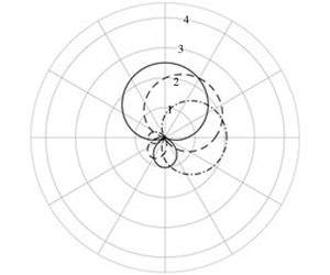
 as is known in sound scattering by a circular cylinder (Lamb Reference Lamb1932). In figure 1, polar plots of  $|{\mathcal{A}}(\unicode[STIX]{x1D703})|$ are shown for
  $f/\unicode[STIX]{x1D714}=0.5$, three different angles of incidence (
 $\unicode[STIX]{x03C0},5\unicode[STIX]{x03C0}/4,3\unicode[STIX]{x03C0}/2$) and
  $b/a=0$, 0.25, 0.50, 0.75 and 1.00, all with the same
  $a$. Since the scattering amplitude increases with the planar area of the island,
  $|{\mathcal{A}}(\unicode[STIX]{x1D703})|$ is the smallest for a thin barrier and greatest for a circle. For the sake of comparison, we present in figure 2 the results for the same set of islands in a non-rotating system. In contrast,
  $|{\mathcal{A}}(\unicode[STIX]{x1D703})|$ is relatively larger and never zero in all directions if
  $f$ is finite.

Figure 1. Scattering amplitude away from islands of different geometries and incidence angles in a rotating sea with  $f/\unicode[STIX]{x1D714}=0.5$, for
  $b/a=0$ (a), 0.25 (b), 0.50 (c), 0.75 (d) and 1.00 (e). Curves represent
  $\unicode[STIX]{x1D703}_{i}=\unicode[STIX]{x03C0}$ (dash–dotted),
  $\unicode[STIX]{x1D703}_{i}=5\unicode[STIX]{x03C0}/4$ (dashed) and
  $\unicode[STIX]{x1D703}_{i}=3\unicode[STIX]{x03C0}/2$ (solid).

Figure 2. Scattering amplitude away from islands of different geometries and incidence angles in a non-rotating fluid  $(f=0)$, for
  $b/a=0$ (a), 0.25 (b), 0.50 (c), 0.75 (d) and 1.00 (e). Curves represent
  $\unicode[STIX]{x1D703}_{i}=\unicode[STIX]{x03C0}$ (dash–dotted),
  $\unicode[STIX]{x1D703}_{i}=5\unicode[STIX]{x03C0}/4$ (dashed) and
  $\unicode[STIX]{x1D703}_{i}=3\unicode[STIX]{x03C0}/2$ (solid).
3.4 Coastal runup
Let us now transform  $(x,y)$ to elliptical coordinates
  $(\unicode[STIX]{x1D707},\unicode[STIX]{x1D708})$ defined by
 $$\begin{eqnarray}z=x+\text{i}y=c\cos (\unicode[STIX]{x1D707}+\text{i}\unicode[STIX]{x1D708})\quad \text{or}\quad x=c\cosh \unicode[STIX]{x1D707}\cos \unicode[STIX]{x1D708},\quad y=c\sinh \unicode[STIX]{x1D707}\sin \unicode[STIX]{x1D708}.\end{eqnarray}$$
 For fixed  $\unicode[STIX]{x1D707}=\unicode[STIX]{x1D707}_{0}$, the point
  $(x,y)$ is on an ellipse with major and minor axes
  $a$ and
  $b$, where
 $$\begin{eqnarray}a=c\cosh \unicode[STIX]{x1D707}_{0},\quad b=c\sinh \unicode[STIX]{x1D707}_{0},\quad a^{2}-b^{2}=c^{2}.\end{eqnarray}$$
The near-field complex potential can be rewritten as
 $$\begin{eqnarray}w(\unicode[STIX]{x1D707}+\text{i}\unicode[STIX]{x1D708})=\unicode[STIX]{x1D719}+\text{i}\unicode[STIX]{x1D713}=U_{0}(a+b)\cosh (\unicode[STIX]{x1D707}-\unicode[STIX]{x1D707}_{0}+\text{i}\unicode[STIX]{x1D708}-\text{i}\unicode[STIX]{x1D703}_{i}),\end{eqnarray}$$
 where  $U+\text{i}V=\bar{U}\text{e}^{\text{i}\unicode[STIX]{x1D703}_{i}}$ with
  $U$ and
  $V$ given by (3.20). On the ellipse
  $\unicode[STIX]{x1D707}=\unicode[STIX]{x1D707}_{0}$,
 $$\begin{eqnarray}x=a\cos \unicode[STIX]{x1D708},\quad y=b\sin \unicode[STIX]{x1D708}=\pm b\sqrt{1-\frac{x^{2}}{a^{2}}},\end{eqnarray}$$
 the stream function  $\unicode[STIX]{x1D713}$ vanishes. The complex potential is
 $$\begin{eqnarray}\displaystyle w(\unicode[STIX]{x1D707}_{0}+\text{i}\unicode[STIX]{x1D708}) & = & \displaystyle \unicode[STIX]{x1D719}=\bar{U}(a+b)\cosh \text{i}(\unicode[STIX]{x1D708}-\unicode[STIX]{x1D703}_{i})=\bar{U}(a+b)\cos (\unicode[STIX]{x1D708}-\unicode[STIX]{x1D703}_{i})\nonumber\\ \displaystyle & = & \displaystyle \bar{U}(a+b)\left[\cos \unicode[STIX]{x1D708}\cos \unicode[STIX]{x1D703}_{i}+\sin \unicode[STIX]{x1D708}\sin \unicode[STIX]{x1D703}_{i}\right].\end{eqnarray}$$
 In particular, the potential on opposite sides of the ellipse  $\left(x,\pm b\sqrt{1-x^{2}/a^{2}}\right)$ is
 $$\begin{eqnarray}\displaystyle \unicode[STIX]{x1D719}_{\pm } & = & \displaystyle \bar{U}(a+b)\left(\cos \unicode[STIX]{x1D708}\cos \unicode[STIX]{x1D703}_{i}+\sin \unicode[STIX]{x1D708}\sin \unicode[STIX]{x1D703}_{i}\right)\nonumber\\ \displaystyle & = & \displaystyle \bar{U}(a+b)\left(\frac{x}{a}\cos \unicode[STIX]{x1D703}_{i}\pm \sqrt{1-\frac{x^{2}}{a^{2}}}\sin \unicode[STIX]{x1D703}_{i}\right).\end{eqnarray}$$
Hence the water-level difference is
 $$\begin{eqnarray}\unicode[STIX]{x0394}\unicode[STIX]{x1D702}=-\frac{\text{i}\unicode[STIX]{x1D714}}{g}(\unicode[STIX]{x1D719}_{+}-\unicode[STIX]{x1D719}_{-})=-\frac{2\text{i}\unicode[STIX]{x1D714}\bar{U}\sin \unicode[STIX]{x1D703}_{i}}{g}(a+b)\sqrt{1-\frac{x^{2}}{a^{2}}},\end{eqnarray}$$
 which is the greatest at  $x=0$ and diminishes to zero at
  $x=\pm a$. Thus, for the same incident tide, the water-level drop is the greatest for a circular island and the smallest for a thin dam. For the same elongated island, the drop is the greatest if the tidal current is normal (
 $\unicode[STIX]{x1D703}_{i}a=\unicode[STIX]{x03C0}/2,\bar{U}\sin \unicode[STIX]{x1D703}_{i}=V$), and is zero if it is parallel (
 $\unicode[STIX]{x1D703}_{i}=0$), to the major axis.
4 Diffraction by a cape
We now turn to a small semi-elliptic cape perpendicular to a straight coast. Let the sea be in the half-plane  $x>0$ and the long axis of the cape be along the
  $x$ axis.
4.1 The incident tide
Two types of ambient tide will be considered.
4.1.1 Reflected Poincaré wave
The surface displacement is
 $$\begin{eqnarray}\unicode[STIX]{x1D701}^{I}=\left(A_{I}\text{e}^{\text{i}\unicode[STIX]{x1D6FC}x}+A_{R}\text{e}^{-\text{i}\unicode[STIX]{x1D6FC}x}\right)\text{e}^{\text{i}\unicode[STIX]{x1D6FD}y},\quad \unicode[STIX]{x1D6FC}^{2}+\unicode[STIX]{x1D6FD}^{2}=k^{2},\end{eqnarray}$$
 where  $A_{I}$ and
  $A_{R}$ are, respectively, the amplitudes of incident and reflected tides. To satisfy the no-flux condition on
  $x=0$, it is necessary that
  $A_{R}$ and
  $A_{I}$ are related by
 $$\begin{eqnarray}A_{R}=A_{I}\frac{\text{i}\unicode[STIX]{x1D714}\unicode[STIX]{x1D6FC}+f\unicode[STIX]{x1D6FD}}{\text{i}\unicode[STIX]{x1D714}\unicode[STIX]{x1D6FC}-f\unicode[STIX]{x1D6FD}}.\end{eqnarray}$$
 Denoting the total wave amplitude along the coast  $x=0$ by
  $A$, then
 $$\begin{eqnarray}A=A_{I}\left(1+\frac{\text{i}\unicode[STIX]{x1D714}\unicode[STIX]{x1D6FC}+f\unicode[STIX]{x1D6FD}}{\text{i}\unicode[STIX]{x1D714}\unicode[STIX]{x1D6FC}-f\unicode[STIX]{x1D6FD}}\right)=A_{I}\frac{2\text{i}\unicode[STIX]{x1D714}\unicode[STIX]{x1D6FC}}{\text{i}\unicode[STIX]{x1D714}\unicode[STIX]{x1D6FC}-f\unicode[STIX]{x1D6FD}}.\end{eqnarray}$$
The ambient tide can be rewritten as
 $$\begin{eqnarray}\unicode[STIX]{x1D701}^{I}=A\left(\frac{\text{i}\unicode[STIX]{x1D714}\unicode[STIX]{x1D6FC}-f\unicode[STIX]{x1D6FD}}{2\text{i}\unicode[STIX]{x1D714}\unicode[STIX]{x1D6FC}}\text{e}^{\text{i}\unicode[STIX]{x1D6FC}x}+\frac{\text{i}\unicode[STIX]{x1D714}\unicode[STIX]{x1D6FC}+f\unicode[STIX]{x1D6FD}}{2\text{i}\unicode[STIX]{x1D714}\unicode[STIX]{x1D6FC}}\text{e}^{-\text{i}\unicode[STIX]{x1D6FC}x}\right)\text{e}^{\text{i}\unicode[STIX]{x1D6FD}y}.\end{eqnarray}$$
From (4.4), the velocity components can be found by using (2.3).
For later matching with the near field, the inner approximation of  $\unicode[STIX]{x1D701}^{I}$ for
  $kr\ll 1$ is
 $$\begin{eqnarray}\displaystyle \frac{\unicode[STIX]{x1D701}_{in}^{I}}{A} & = & \displaystyle 1-\frac{f\unicode[STIX]{x1D6FD}}{\unicode[STIX]{x1D714}}x+\text{i}\unicode[STIX]{x1D6FD}y-\frac{1}{2}(\unicode[STIX]{x1D6FC}^{2}x^{2}+\unicode[STIX]{x1D6FD}^{2}y^{2})-\text{i}\frac{f}{\unicode[STIX]{x1D714}}\unicode[STIX]{x1D6FD}^{2}xy+O(k^{3}a^{3}).\end{eqnarray}$$
Again, both linear and quadratic terms are kept in (4.5) for later determination of the scattered wave in the outer field.
Corresponding to the linear terms above, the leading-order inner approximation of the incoming current near the cape is
 $$\begin{eqnarray}u^{I}(0,0)\approx 0,\quad v^{I}(0,0)\approx -\frac{gA\unicode[STIX]{x1D6FD}}{\unicode[STIX]{x1D714}}.\end{eqnarray}$$
Thus the tidal current is essentially parallel to the coast.
4.1.2 Kelvin wave
Propagating along the coast, the Kelvin wave is given by
 $$\begin{eqnarray}\unicode[STIX]{x1D701}^{I}=A\text{e}^{(-fx+\text{i}\unicode[STIX]{x1D714}y)/C},\end{eqnarray}$$
 with  $C=\sqrt{gh}$. In the near field,
  $kr\ll 1$,
 $$\begin{eqnarray}\displaystyle \unicode[STIX]{x1D701}_{in}^{I}\approx A\left[1-\frac{fx}{C}+\frac{\text{i}\unicode[STIX]{x1D714}y}{C}+\frac{1}{2C^{2}}\left(f^{2}x^{2}-\unicode[STIX]{x1D714}^{2}y^{2}\right)-\text{i}\frac{f}{\unicode[STIX]{x1D714}}\unicode[STIX]{x1D6FD}^{2}xy+O(k^{3}a^{3})+\cdots \right]. & & \displaystyle\end{eqnarray}$$
The corresponding tidal current has the components
 $$\begin{eqnarray}u_{in}^{I}\approx 0\quad \text{and}\quad v_{in}^{I}\approx -\frac{A}{h}\sqrt{gh}=\text{const.}\end{eqnarray}$$
and is parallel to the coast.
4.2 The outer solution
In his theory of tidal diffraction by a coastal estuary, Buchwald (Reference Buchwald1971) derived by Fourier transform the Green’s function which represents a point source at the origin. To account for the scattering effects of a small island, we approximate the scattered wave by the sum of a source and a doublet,
 $$\begin{eqnarray}\unicode[STIX]{x1D701}\approx \unicode[STIX]{x1D701}^{I}+C_{0}G+D\frac{\unicode[STIX]{x2202}G}{\unicode[STIX]{x2202}y},\end{eqnarray}$$
 where  $C_{0}$ and
  $D$ are the unknown strengths of the source and doublet, respectively. We have replaced Buchwald’s Green’s function
  $\unicode[STIX]{x1D701}_{G}$ by
  $G$ defined by
  $\unicode[STIX]{x1D701}_{G}=(\unicode[STIX]{x1D714}/2g)G$. It can be shown that the need for
  $\unicode[STIX]{x2202}G/\unicode[STIX]{x2202}x$ does not arise. Buchwald has given the approximations of
  $G$ valid for both the far field
  $kr\gg 1$ and the near field
  $kr\ll 1$ and for both
  $\unicode[STIX]{x1D70E}=\unicode[STIX]{x1D714}/f>1$ and
  $\unicode[STIX]{x1D70E}=\unicode[STIX]{x1D714}/f<1$. We shall focus our discussion on diurnal tides and the northern hemisphere with
  $\unicode[STIX]{x1D70E}=\unicode[STIX]{x1D714}/f>1$.
4.2.1 The far field $(kr\gg 1)$

For  $\unicode[STIX]{x1D714}>f$, Buchwald has derived the far field of the source to be
 $$\begin{eqnarray}G\approx G_{K}\text{H}(\unicode[STIX]{x1D703}_{0}-\unicode[STIX]{x1D703})+G_{P},\end{eqnarray}$$
 where  $\text{H}(\unicode[STIX]{x1D703}_{0}-\unicode[STIX]{x1D703})$ denotes the Heaviside function with
 $$\begin{eqnarray}\unicode[STIX]{x1D703}_{0}=-\sin ^{-1}(kC/\unicode[STIX]{x1D714})=-\sin \sqrt{1-\frac{f^{2}}{\unicode[STIX]{x1D714}^{2}}},\end{eqnarray}$$
 $G_{K}$ is the Kelvin wave given by
 $$\begin{eqnarray}G_{K}=\frac{2f}{\unicode[STIX]{x1D714}}\text{e}^{(\text{i}\unicode[STIX]{x1D714}y-fx)/C}\end{eqnarray}$$
 and  $G_{P}$ denotes the Poincaré wave
 $$\begin{eqnarray}G_{P}=\frac{\unicode[STIX]{x1D714}^{2}-f^{2}}{\unicode[STIX]{x1D714}^{2}}\left(\frac{2}{\unicode[STIX]{x03C0}kr}\right)^{1/2}\frac{\cos \unicode[STIX]{x1D703}}{\cos \unicode[STIX]{x1D703}-\text{i}(f/\unicode[STIX]{x1D714})\sin \unicode[STIX]{x1D703}}\text{e}^{-\text{i}(kr-\unicode[STIX]{x03C0}/4)}+O((kr)^{-3/2}),\end{eqnarray}$$
 where  $(r,\unicode[STIX]{x1D703})$ are the polar coordinates.
Since
 $$\begin{eqnarray}\frac{\unicode[STIX]{x2202}}{\unicode[STIX]{x2202}y}=\sin \unicode[STIX]{x1D703}\frac{\unicode[STIX]{x2202}}{\unicode[STIX]{x2202}r}+\frac{\cos \unicode[STIX]{x1D703}}{r}\frac{\unicode[STIX]{x2202}}{\unicode[STIX]{x2202}\unicode[STIX]{x1D703}}=\frac{y}{r}\frac{\unicode[STIX]{x2202}}{\unicode[STIX]{x2202}r}+\frac{x}{r^{2}}\frac{\unicode[STIX]{x2202}}{\unicode[STIX]{x2202}\unicode[STIX]{x1D703}},\end{eqnarray}$$
the far field of the doublet is
 $$\begin{eqnarray}\displaystyle D\frac{\unicode[STIX]{x2202}G}{\unicode[STIX]{x2202}y} & {\approx} & \displaystyle D\left\{\vphantom{\sqrt{\frac{2}{\unicode[STIX]{x03C0}kr}}}2\text{i}f\text{e}^{(\text{i}\unicode[STIX]{x1D714}y-fx)/C}\text{H}(\unicode[STIX]{x1D703}_{0}-\unicode[STIX]{x1D703})\right.\nonumber\\ \displaystyle & & \displaystyle \left.-\text{i}k\frac{\unicode[STIX]{x1D714}^{2}-f^{2}}{\unicode[STIX]{x1D714}^{2}}\sqrt{\frac{2}{\unicode[STIX]{x03C0}kr}}\frac{y}{r}\frac{\cos \unicode[STIX]{x1D703}}{\cos \unicode[STIX]{x1D703}-\text{i}(f/\unicode[STIX]{x1D714})\sin \unicode[STIX]{x1D703}}\text{e}^{-\text{i}(kr-\unicode[STIX]{x03C0}/4)}\right\}+O(kr)^{-3/2}.\qquad\end{eqnarray}$$
The total scattered wave in the outer field is
 $$\begin{eqnarray}\displaystyle \unicode[STIX]{x1D701}^{S} & {\approx} & \displaystyle \left(C_{0}\frac{2f}{\unicode[STIX]{x1D714}}+D\frac{2\text{i}f}{C}\right)\text{e}^{(\text{i}\unicode[STIX]{x1D714}y-fx)/C}\text{H}(\unicode[STIX]{x1D703}_{0}-\unicode[STIX]{x1D703})\nonumber\\ \displaystyle & & \displaystyle +\,(C_{0}-\text{i}kD\sin \unicode[STIX]{x1D703})\left\{\frac{\unicode[STIX]{x1D714}^{2}-f^{2}}{\unicode[STIX]{x1D714}^{2}}\sqrt{\frac{2}{\unicode[STIX]{x03C0}kr}}\frac{\cos \unicode[STIX]{x1D703}}{\cos \unicode[STIX]{x1D703}-\text{i}(f/\unicode[STIX]{x1D714})\sin \unicode[STIX]{x1D703}}\text{e}^{-\text{i}(kr-\unicode[STIX]{x03C0}/4)}\right\}\!.\qquad\end{eqnarray}$$
 The physics is an extension to that described by Buchwald. In particular,  $\unicode[STIX]{x1D703}_{0}\rightarrow -\unicode[STIX]{x03C0}/2$ for
  $f/\unicode[STIX]{x1D714}\rightarrow 1$; no Kelvin wave is produced. On the other hand,
  $\unicode[STIX]{x1D703}_{0}\rightarrow 0$ if
  $f/\unicode[STIX]{x1D714}\rightarrow 1$ from below; a Kelvin wave is present for all
  $y<0$. The intensity of the Poincaré wave varies with direction differently, being the weakest in directions parallel and normal to the coast (
 $\unicode[STIX]{x1D703}=0,\pm \unicode[STIX]{x03C0}/2$), and strongest along
  $\unicode[STIX]{x1D703}=\pm \unicode[STIX]{x03C0}/4$.
The coefficients  $C_{0}$ and
  $D$ will now be determined by matching the small-
 $kr$ approximation of the outer solution (the wave field) with the large-
 $z/a$ approximation of the near field.
For matching with the inner solution, we need only the following inner approximations given by Buchwald (Reference Buchwald1971). Focusing on  $\unicode[STIX]{x1D714}>f$ only,
 $$\begin{eqnarray}G\approx \frac{\unicode[STIX]{x1D714}}{2g}\left[1-\frac{2\text{i}}{\unicode[STIX]{x03C0}}\log \frac{\unicode[STIX]{x1D6FE}kr}{2}-\frac{1}{\unicode[STIX]{x03C0}\unicode[STIX]{x1D70E}}\left(2\unicode[STIX]{x1D703}+\text{i}\log \frac{\unicode[STIX]{x1D70E}+1}{\unicode[STIX]{x1D70E}-1}\right)\right]+O(kr),\quad \unicode[STIX]{x1D70E}=\frac{\unicode[STIX]{x1D714}}{f}.\end{eqnarray}$$
 It is easy to find for  $kr\ll 1$ that
 $$\begin{eqnarray}\displaystyle \frac{\unicode[STIX]{x2202}G}{\unicode[STIX]{x2202}y}\approx \left\{\sin \unicode[STIX]{x1D703}\left(-\frac{2\text{i}}{\unicode[STIX]{x03C0}r}\right)+\frac{\cos \unicode[STIX]{x1D703}}{r}\left(\frac{-2}{\unicode[STIX]{x03C0}\unicode[STIX]{x1D70E}}\right)\right\}=-\frac{2\text{i}}{\unicode[STIX]{x03C0}}\frac{y}{r^{2}}-\frac{2}{\unicode[STIX]{x03C0}\unicode[STIX]{x1D70E}}\frac{x}{r^{2}}. & & \displaystyle\end{eqnarray}$$
The inner approximation of the outer solution is, for the incident and reflected Poincaré wave,
 $$\begin{eqnarray}\displaystyle \unicode[STIX]{x1D701} & {\approx} & \displaystyle \unicode[STIX]{x1D701}^{I}+C_{0}G+D\frac{\unicode[STIX]{x2202}G}{\unicode[STIX]{x2202}y}\nonumber\\ \displaystyle & {\approx} & \displaystyle A+\frac{\unicode[STIX]{x1D6FD}A}{\unicode[STIX]{x1D714}}\left(\text{i}\unicode[STIX]{x1D714}y-fx\right)\nonumber\\ \displaystyle & & \displaystyle +\,C_{0}\left(1-\frac{2\text{i}}{\unicode[STIX]{x03C0}}\log \frac{\unicode[STIX]{x1D6FE}kr}{2}\right)+D\left\{-\frac{2\text{i}}{\unicode[STIX]{x03C0}}\frac{y}{r^{2}}-\frac{2}{\unicode[STIX]{x03C0}\unicode[STIX]{x1D70E}}\frac{x}{r^{2}}\right\},\quad kr\ll 1,\end{eqnarray}$$
and for the Kelvin tide,
 $$\begin{eqnarray}\displaystyle \unicode[STIX]{x1D701} & {\approx} & \displaystyle \unicode[STIX]{x1D701}^{I}+C_{0}G+D\frac{\unicode[STIX]{x2202}G}{\unicode[STIX]{x2202}y}\nonumber\\ \displaystyle & {\approx} & \displaystyle A-A\frac{f}{\sqrt{gh}}x+A\frac{\text{i}\unicode[STIX]{x1D714}}{\sqrt{gh}}y\nonumber\\ \displaystyle & & \displaystyle +\,C_{0}\left(1-\frac{2\text{i}}{\unicode[STIX]{x03C0}}\log \frac{\unicode[STIX]{x1D6FE}kr}{2}\right)+D\left\{-\frac{2\text{i}}{\unicode[STIX]{x03C0}}\frac{y}{r^{2}}-\frac{2}{\unicode[STIX]{x03C0}\unicode[STIX]{x1D70E}}\frac{x}{r^{2}}\right\},\quad kr\ll 1.\end{eqnarray}$$
4.3 Matching with the near field
The near field (inner solution, again denoted by  $\unicode[STIX]{x1D702}$) can be obtained from § 3.2 by taking
  $U=0$ and
  $V\neq 0$ in (4.6) or (4.9).
In particular, the outer approximation of the inner solution  $\unicode[STIX]{x1D702}$ is
 $$\begin{eqnarray}\displaystyle \unicode[STIX]{x1D702}_{out} & = & \displaystyle -\frac{1}{g}\left(\text{i}\unicode[STIX]{x1D714}\unicode[STIX]{x1D719}+f\unicode[STIX]{x1D713}\right)_{out}\nonumber\\ \displaystyle & = & \displaystyle -\frac{1}{g}\left\{-f\,Vx+\text{i}\unicode[STIX]{x1D714}Vy\right\}-\frac{1}{g}\frac{Va(a+b)}{2r^{2}}(fx+\text{i}\unicode[STIX]{x1D714}y),\quad \frac{r}{c}\gg 1.\end{eqnarray}$$
4.3.1 Reflected Poincaré tide
For the reflected Poincaré tide, we match the coefficients of  $x$ in (4.22) and (4.20):
 $$\begin{eqnarray}\frac{f\,V}{g}=-f\frac{\unicode[STIX]{x1D6FD}A}{\unicode[STIX]{x1D714}},\quad \text{hence}\quad V=-\frac{g\unicode[STIX]{x1D6FD}A}{\unicode[STIX]{x1D714}},\end{eqnarray}$$
 as in (4.6). The same result is obtained by matching the coefficients of  $y$ in the same equations.
Matching the coefficients of  $x/r^{2}$,
 $$\begin{eqnarray}-\frac{1}{g}\frac{Va(a+b)}{2}f=-\frac{2f}{\unicode[STIX]{x03C0}\unicode[STIX]{x1D714}}D,\end{eqnarray}$$
 and the coefficients of  $y/r^{2}$,
 $$\begin{eqnarray}-\frac{1}{g}\frac{Va(a+b)}{2}\text{i}\unicode[STIX]{x1D714}=-D\frac{2\text{i}}{\unicode[STIX]{x03C0}},\end{eqnarray}$$
we get the same doublet strength:
 $$\begin{eqnarray}D=\frac{\unicode[STIX]{x1D714}}{4g}\unicode[STIX]{x03C0}a(a+b)V=-\frac{\unicode[STIX]{x1D714}}{4g}\unicode[STIX]{x03C0}a(a+b)\frac{g\unicode[STIX]{x1D6FD}A}{\unicode[STIX]{x1D714}}=-\frac{\unicode[STIX]{x03C0}ka(a+b)}{4}\frac{\unicode[STIX]{x1D6FD}}{k}A.\end{eqnarray}$$
4.3.2 Kelvin tide
For the Kelvin tide, matching the coefficients of  $x$ and
  $y$ in (4.22) and (4.21) gives
 $$\begin{eqnarray}\frac{f\,V}{g}=-\frac{fA}{\sqrt{gh}}\quad \text{and}\quad -\frac{\text{i}\unicode[STIX]{x1D714}V}{g}=\frac{\text{i}\unicode[STIX]{x1D714}A}{\sqrt{gh}},\end{eqnarray}$$
which leads to the same result,
 $$\begin{eqnarray}V=-\frac{gA}{\sqrt{gh}}.\end{eqnarray}$$
 Matching the coefficients of  $x/r^{2}$ or
  $y/r^{2}$ gives
 $$\begin{eqnarray}-\frac{Df}{\unicode[STIX]{x03C0}g}=-\frac{f\,Va(a+b)}{2g},\quad -D\frac{2\text{i}}{\unicode[STIX]{x03C0}}=-\text{i}\unicode[STIX]{x1D714}V\frac{a(a+b)}{2g},\end{eqnarray}$$
 which gives the same result for  $D$. Since
  $V=-gA/\sqrt{gh}=-gA/C$, we have
 $$\begin{eqnarray}\displaystyle D=\frac{\unicode[STIX]{x03C0}\unicode[STIX]{x1D714}Va(a+b)}{4g}=-\frac{\unicode[STIX]{x03C0}ka(a+b)}{4}A\frac{\unicode[STIX]{x1D714}}{kC}. & & \displaystyle\end{eqnarray}$$
Thus the doublet strength is different from (4.26).
4.4 The source strength $C_{0}$

We invoke Rayleigh’s argument by finding first the tide influx repelled by the cape. Let  $\unicode[STIX]{x2202}S$ be a semicircle surrounding the cape. By using the orthogonal elliptic coordinates
  $\unicode[STIX]{x1D707},\unicode[STIX]{x1D708}$ defined by
  $x+\text{i}y=c\cos (\unicode[STIX]{x1D707}+\text{i}\unicode[STIX]{x1D708})$, it is shown in appendix B that (3.29) is equivalent to
 $$\begin{eqnarray}k^{2}h\int _{\unicode[STIX]{x2202}S}\boldsymbol{u}_{in}^{I}\boldsymbol{\cdot }\boldsymbol{n}\,\text{d}s=\text{i}\unicode[STIX]{x1D714}\int _{\unicode[STIX]{x2202}S}\frac{\unicode[STIX]{x2202}\unicode[STIX]{x1D701}_{in}^{I}}{\unicode[STIX]{x2202}\unicode[STIX]{x1D707}}\,\text{d}\unicode[STIX]{x1D708}+f\int _{\unicode[STIX]{x2202}S}\frac{\unicode[STIX]{x2202}\unicode[STIX]{x1D701}_{in}^{I}}{\unicode[STIX]{x2202}\unicode[STIX]{x1D708}}\,\text{d}\unicode[STIX]{x1D708}.\end{eqnarray}$$
 The line integrals above must be evaluated for Poincaré tide and Kelvin tide by using the quadratic part  $\unicode[STIX]{x1D701}_{in,2}^{I}$ in (4.5) and (4.8), respectively, for
  $\unicode[STIX]{x1D701}_{in}^{I}$.
4.4.1 Reflected Poincaré tide
From (4.5), the second-order part of  $\unicode[STIX]{x1D701}_{in}^{I}$ is
 $$\begin{eqnarray}\displaystyle \hspace{-24.0pt}\unicode[STIX]{x1D701}_{in,2}^{I} & = & \displaystyle -\frac{A}{2}c^{2}(\unicode[STIX]{x1D6FC}^{2}\cosh ^{2}\unicode[STIX]{x1D707}\cos ^{2}\unicode[STIX]{x1D708}+\unicode[STIX]{x1D6FD}^{2}\sinh ^{2}\unicode[STIX]{x1D707}\sin ^{2}\unicode[STIX]{x1D708})\nonumber\\ \displaystyle \hspace{-24.0pt} & & \displaystyle -\,\text{i}A\frac{f}{\unicode[STIX]{x1D714}}\unicode[STIX]{x1D6FD}^{2}c^{2}\cosh \unicode[STIX]{x1D707}\cosh \unicode[STIX]{x1D708}\sinh \unicode[STIX]{x1D707}\sin \unicode[STIX]{x1D708}\nonumber\\ \displaystyle \hspace{-24.0pt} & = & \displaystyle -\frac{A}{2}c^{2}(\unicode[STIX]{x1D6FC}^{2}\cosh ^{2}\unicode[STIX]{x1D707}\cos ^{2}\unicode[STIX]{x1D708}+\unicode[STIX]{x1D6FD}^{2}\sinh ^{2}\unicode[STIX]{x1D707}\sin ^{2}\unicode[STIX]{x1D708})-\text{i}A\frac{f}{4\unicode[STIX]{x1D714}}\unicode[STIX]{x1D6FD}^{2}c^{2}\sinh 2\unicode[STIX]{x1D707}\sin 2\unicode[STIX]{x1D708}.\end{eqnarray}$$
 Referring to (4.31), we get, on the ellipse,  $\unicode[STIX]{x1D707}=\unicode[STIX]{x1D707}_{0}$,
 $$\begin{eqnarray}\displaystyle \int _{-\unicode[STIX]{x03C0}/2}^{\unicode[STIX]{x03C0}/2}\text{d}\unicode[STIX]{x1D708}\,\frac{\unicode[STIX]{x2202}\unicode[STIX]{x1D701}_{in,2}^{I}}{\unicode[STIX]{x2202}\unicode[STIX]{x1D707}} & = & \displaystyle -Ac^{2}\cosh \unicode[STIX]{x1D707}_{0}\sinh \unicode[STIX]{x1D707}_{0}\int _{-\unicode[STIX]{x03C0}/2}^{\unicode[STIX]{x03C0}/2}\text{d}\unicode[STIX]{x1D708}\,(\unicode[STIX]{x1D6FC}^{2}\cos ^{2}\unicode[STIX]{x1D708}+\unicode[STIX]{x1D6FD}^{2}\sin ^{2}\unicode[STIX]{x1D708})\nonumber\\ \displaystyle & & \displaystyle -\,\text{i}A\frac{f}{2\unicode[STIX]{x1D714}}\unicode[STIX]{x1D6FD}^{2}c^{2}\cosh 2\unicode[STIX]{x1D707}_{0}\int _{-\unicode[STIX]{x03C0}/2}^{\unicode[STIX]{x03C0}/2}\sin 2\unicode[STIX]{x1D708}\,\text{d}\unicode[STIX]{x1D6FE}\nonumber\\ \displaystyle & = & \displaystyle -Aab\left[\unicode[STIX]{x1D6FC}^{2}\left(\frac{\unicode[STIX]{x1D708}}{2}-\frac{\sin 2\unicode[STIX]{x1D708}}{4}\right)+\unicode[STIX]{x1D6FD}^{2}\left(\frac{\unicode[STIX]{x1D708}}{2}+\frac{\sin 2\unicode[STIX]{x1D708}}{4}\right)\right]_{-\unicode[STIX]{x03C0}/2}^{\unicode[STIX]{x03C0}/2}\nonumber\\ \displaystyle & = & \displaystyle -Aab(\unicode[STIX]{x1D6FC}^{2}+\unicode[STIX]{x1D6FD}^{2})\frac{\unicode[STIX]{x03C0}}{2}=-A\frac{\unicode[STIX]{x03C0}k^{2}ab}{2},\end{eqnarray}$$
 $$\begin{eqnarray}\displaystyle \int _{-\unicode[STIX]{x03C0}/2}^{\unicode[STIX]{x03C0}/2}\text{d}\unicode[STIX]{x1D708}\,\frac{\unicode[STIX]{x2202}\unicode[STIX]{x1D701}_{in,2}^{I}}{\unicode[STIX]{x2202}\unicode[STIX]{x1D708}} & = & \displaystyle A(\unicode[STIX]{x1D6FC}^{2}\cosh ^{2}\unicode[STIX]{x1D707}-\unicode[STIX]{x1D6FD}^{2}\sinh ^{2}\unicode[STIX]{x1D707})\int _{-\unicode[STIX]{x03C0}/2}^{\unicode[STIX]{x03C0}/2}\text{d}\unicode[STIX]{x1D708}\,\frac{1}{2}\sin 2\unicode[STIX]{x1D708}\nonumber\\ \displaystyle & = & \displaystyle \frac{A}{4}A(\unicode[STIX]{x1D6FC}^{2}\cosh ^{2}\unicode[STIX]{x1D707}-\unicode[STIX]{x1D6FD}^{2}\sinh ^{2}\unicode[STIX]{x1D707})[\cos 2\unicode[STIX]{x1D708}]_{-\unicode[STIX]{x03C0}/2}^{\unicode[STIX]{x03C0}/2}=0.\end{eqnarray}$$
Hence the flux that the incoming tide pushes towards the cape is
 $$\begin{eqnarray}M_{in}=-\frac{\text{i}\unicode[STIX]{x1D714}}{k^{2}h}\int _{-\unicode[STIX]{x03C0}/2}^{\unicode[STIX]{x03C0}/2}\text{d}\unicode[STIX]{x1D708}\,\frac{\unicode[STIX]{x2202}\unicode[STIX]{x1D701}_{in,2}^{I}}{\unicode[STIX]{x2202}\unicode[STIX]{x1D707}}=\frac{\text{i}\unicode[STIX]{x1D714}}{k^{2}h}\frac{\unicode[STIX]{x03C0}Ak^{2}ab}{2}.\end{eqnarray}$$
 Across a semicircle at the outer limit of the inner region,  $r/a\gg 1$, the total repelling flux is, from (4.20),
 $$\begin{eqnarray}M_{out}=\frac{\text{i}\unicode[STIX]{x1D714}}{k^{2}h}\unicode[STIX]{x03C0}r\frac{\unicode[STIX]{x2202}\unicode[STIX]{x1D701}_{0}^{S}}{\unicode[STIX]{x2202}r}\approx \frac{\text{i}\unicode[STIX]{x1D714}}{k^{2}h}\unicode[STIX]{x03C0}r\frac{\unicode[STIX]{x2202}}{\unicode[STIX]{x2202}r}\left(C_{0}-C_{0}\frac{2\text{i}}{\unicode[STIX]{x03C0}}\ln \frac{kr}{2}\right)=-\frac{\text{i}\unicode[STIX]{x1D714}}{k^{2}h}C_{0}\frac{2\text{i}\unicode[STIX]{x1D714}}{2g},\end{eqnarray}$$
 which is one-half of (3.33). It follows by requiring  $M_{in}=M_{out}$ that
 $$\begin{eqnarray}C_{0}=\frac{\text{i}A}{4}\unicode[STIX]{x03C0}k^{2}ab.\end{eqnarray}$$
 Again,  $C_{0}$ is the largest for a circle (
 $b=a$) and zero for a thin barrier (
 $b=0$).
In summary the outer tidal field is given by (4.10) with the ambient tide given by (4.4), the source strength by (4.37) and the doublet strength by (4.26).
4.4.2 Kelvin tide
For the Kelvin tide incident from the north,  $\unicode[STIX]{x1D6FD}=0$, the second-order part is, from (4.8),
 $$\begin{eqnarray}\unicode[STIX]{x1D701}_{in,2}^{I}=\frac{A}{2C^{2}}\left(f^{2}x^{2}-\unicode[STIX]{x1D714}^{2}y^{2}\right)=\frac{Ac^{2}}{2C^{2}}\left(f^{2}\cosh ^{2}\unicode[STIX]{x1D707}\cos ^{2}\unicode[STIX]{x1D708}-\unicode[STIX]{x1D714}^{2}\sinh ^{2}\unicode[STIX]{x1D707}\sin ^{2}\unicode[STIX]{x1D708}\right).\end{eqnarray}$$
 On the semi-ellipse,  $\unicode[STIX]{x1D707}=\unicode[STIX]{x1D707}_{0}$,
 $$\begin{eqnarray}\displaystyle \int _{-\unicode[STIX]{x03C0}/2}^{\unicode[STIX]{x03C0}/2}\text{d}\unicode[STIX]{x1D708}\,\frac{\unicode[STIX]{x2202}\unicode[STIX]{x1D701}_{2}^{I}}{\unicode[STIX]{x2202}\unicode[STIX]{x1D707}} & = & \displaystyle \int _{-\unicode[STIX]{x03C0}/2}^{\unicode[STIX]{x03C0}/2}\text{d}\unicode[STIX]{x1D708}\,\frac{Ac^{2}}{C^{2}}\sinh \unicode[STIX]{x1D707}_{0}\cosh \unicode[STIX]{x1D707}_{0}(f^{2}\cos ^{2}\unicode[STIX]{x1D708}-\unicode[STIX]{x1D714}^{2}\sin ^{2}\unicode[STIX]{x1D708})\nonumber\\ \displaystyle & = & \displaystyle -\frac{A}{2C^{2}}\unicode[STIX]{x03C0}ab(\unicode[STIX]{x1D714}^{2}-f^{2})=-\frac{A}{2}\unicode[STIX]{x03C0}k^{2}ab\end{eqnarray}$$
and
 $$\begin{eqnarray}\int _{-\unicode[STIX]{x03C0}/2}^{\unicode[STIX]{x03C0}/2}\text{d}\unicode[STIX]{x1D708}\,\frac{\unicode[STIX]{x2202}\unicode[STIX]{x1D701}_{2}^{I}}{\unicode[STIX]{x2202}\unicode[STIX]{x1D708}}=-\frac{1}{2}\frac{Ac^{2}}{gh}(\unicode[STIX]{x1D714}^{2}\sinh ^{2}\unicode[STIX]{x1D707}_{0}-f^{2}\cosh ^{2}\unicode[STIX]{x1D707}_{0})\int _{-\unicode[STIX]{x03C0}/2}^{\unicode[STIX]{x03C0}/2}\text{d}\unicode[STIX]{x1D708}\,\sin 2\unicode[STIX]{x1D708}=0.\end{eqnarray}$$
Again
 $$\begin{eqnarray}\frac{\text{i}\unicode[STIX]{x1D714}}{k^{2}h}\frac{A}{2}\unicode[STIX]{x03C0}k^{2}ab=M_{in}.\end{eqnarray}$$
From (4.21), the outflux through a semicircle is still given by (4.36). Upon equating the influx and and outflux, we get
 $$\begin{eqnarray}C_{0}=\frac{\text{i}A}{4}\unicode[STIX]{x03C0}k^{2}ab.\end{eqnarray}$$
In summary, the outer tidal field is given by (4.10) with the ambient tide given by (4.7), the source strength by (4.42) and the doublet strength by (4.30). The two ambient waves lead to the same source strength but different doublet strengths.
4.5 Scattered wave pattern in the far field
We summarize below the scattering amplitudes for the two incident tides.
4.5.1 Incident Poincaré tide
Using (4.26) and (4.37), we get
 $$\begin{eqnarray}\displaystyle C_{0}\frac{2f}{\unicode[STIX]{x1D714}}+D\frac{2\text{i}f}{C} & = & \displaystyle \text{i}A\frac{f}{\unicode[STIX]{x1D714}}\frac{\unicode[STIX]{x03C0}k^{2}ab}{2}-\text{i}A\frac{f}{kC}\frac{\unicode[STIX]{x03C0}k^{2}a(a+b)}{2}\frac{\unicode[STIX]{x1D6FD}}{k}\nonumber\\ \displaystyle & = & \displaystyle \frac{\text{i}A\unicode[STIX]{x03C0}k^{2}a^{2}}{2}\frac{f}{\unicode[STIX]{x1D714}}\left[\frac{b}{a}-\frac{\unicode[STIX]{x1D714}}{kC}\frac{\unicode[STIX]{x1D6FD}}{k}\left(1+\frac{b}{a}\right)\right].\quad\end{eqnarray}$$
Let us define the directional factor of the scattered Kelvin wave by
 $$\begin{eqnarray}\displaystyle {\mathcal{A}}_{KP} & = & \displaystyle \frac{f}{\unicode[STIX]{x1D714}}\left\{\frac{b}{a}-\frac{\unicode[STIX]{x1D714}}{kC}\frac{\unicode[STIX]{x1D6FD}}{k}\left(1+\frac{b}{a}\right)\right\}=\frac{f}{\unicode[STIX]{x1D714}}\left\{\frac{b}{a}+\frac{\sin \unicode[STIX]{x1D703}_{i}}{\sqrt{1-f^{2}/\unicode[STIX]{x1D714}^{2}}}\left(1+\frac{b}{a}\right)\right\}.\quad\end{eqnarray}$$
Since
 $$\begin{eqnarray}\displaystyle C_{0}-\text{i}kD\sin \unicode[STIX]{x1D703} & = & \displaystyle \frac{\text{i}A\unicode[STIX]{x03C0}k^{2}ab}{4}-\text{i}k\frac{-\unicode[STIX]{x03C0}ka(a+b)}{4}\frac{\unicode[STIX]{x1D6FD}}{k}A\sin \unicode[STIX]{x1D703}\nonumber\\ \displaystyle & = & \displaystyle \frac{\text{i}A\unicode[STIX]{x03C0}k^{2}a^{2}}{4}\left[\frac{b}{a}-\left(1+\frac{b}{a}\right)\sin \unicode[STIX]{x1D703}_{i}\sin \unicode[STIX]{x1D703}\right],\quad\end{eqnarray}$$
the amplitude of the scattered Poincaré wave is
 $$\begin{eqnarray}\displaystyle & & \displaystyle \frac{\text{i}A\unicode[STIX]{x03C0}k^{2}a^{2}}{4}\frac{\unicode[STIX]{x1D714}^{2}-f^{2}}{\unicode[STIX]{x1D714}^{2}}\left[\frac{b}{a}-\left(1+\frac{b}{a}\right)\sin \unicode[STIX]{x1D703}_{i}\sin \unicode[STIX]{x1D703}\right]\frac{\cos \unicode[STIX]{x1D703}}{\cos \unicode[STIX]{x1D703}-\text{i}(f/\unicode[STIX]{x1D714})\sin \unicode[STIX]{x1D703}_{i}\sin \unicode[STIX]{x1D703}}\nonumber\\ \displaystyle & & \displaystyle \quad =\frac{\text{i}A\unicode[STIX]{x03C0}k^{2}a^{2}}{4}{\mathcal{A}}_{PP},\end{eqnarray}$$
where
 $$\begin{eqnarray}{\mathcal{A}}_{PP}(\unicode[STIX]{x1D703})=\left(1-\frac{f^{2}}{\unicode[STIX]{x1D714}^{2}}\right)\left[\frac{b}{a}-\left(1+\frac{b}{a}\right)\sin \unicode[STIX]{x1D703}_{i}\sin \unicode[STIX]{x1D703}\right]\frac{\cos \unicode[STIX]{x1D703}}{\cos \unicode[STIX]{x1D703}-\text{i}(f/\unicode[STIX]{x1D714})\sin \unicode[STIX]{x1D703}}\end{eqnarray}$$
represents the directional pattern of the scattered Poincaré wave. The magnitude
 $$\begin{eqnarray}|{\mathcal{A}}_{PP}(\unicode[STIX]{x1D703})|=\left(1-\frac{f^{2}}{\unicode[STIX]{x1D714}^{2}}\right)\left[\frac{b}{a}-\left(1+\frac{b}{a}\right)\sin \unicode[STIX]{x1D703}_{i}\sin \unicode[STIX]{x1D703}\right]\frac{\cos \unicode[STIX]{x1D703}}{\sqrt{\cos ^{2}\unicode[STIX]{x1D703}+(f^{2}/\unicode[STIX]{x1D714}^{2})\sin ^{2}\unicode[STIX]{x1D703}}}\end{eqnarray}$$
 is larger for smaller  $f/\unicode[STIX]{x1D714}$.
We display the numerical results for  $|{\mathcal{A}}_{PP}(\unicode[STIX]{x1D703})|$ in figure 3 for
  $\unicode[STIX]{x1D703}_{i}=5\unicode[STIX]{x03C0}/4$ and for several different
  $f/\unicode[STIX]{x1D714}$ and
  $b/a$. While the extrema are at
  $\unicode[STIX]{x1D703}=\pm \unicode[STIX]{x03C0}/2$ for
  $f/\unicode[STIX]{x1D714}=0$, they are shifted to
  $\unicode[STIX]{x1D703}=\pm \unicode[STIX]{x03C0}/4$.

Figure 3. Directional pattern of scattered Poincaré wave  $|{\mathcal{A}}_{PP}|$ for a cape, for
  $f/\unicode[STIX]{x1D714}=0$ (a), 0.30 (b) and 0.60 (c). Direction of incident Poincaré wave:
  $\unicode[STIX]{x1D703}_{i}=5\unicode[STIX]{x03C0}/4$. Curves represent
  $b/a=0$ (dash–dotted),
  $b/a=0.50$ (dashed) and
  $b/a=1.00$ (solid).
4.5.2 Kelvin tide
Using (4.42) and (4.30), the amplitude of the scattered Kelvin wave is
 $$\begin{eqnarray}\displaystyle \hspace{-12.0pt}C_{0}\left(\frac{2f}{\unicode[STIX]{x1D714}}\right)+D\left(\frac{2\text{i}f}{C}\right) & = & \displaystyle \frac{\text{i}A\unicode[STIX]{x03C0}k^{2}ab}{4}\left(\frac{2f}{\unicode[STIX]{x1D714}}\right)-\frac{\unicode[STIX]{x03C0}k^{2}a(a+b)}{4}\frac{\unicode[STIX]{x1D714}}{kC}A\left(\frac{2\text{i}f}{\unicode[STIX]{x1D714}}\right)\nonumber\\ \displaystyle \hspace{-12.0pt} & = & \displaystyle \frac{\text{i}A\unicode[STIX]{x03C0}k^{2}a^{2}}{2}\frac{f}{\unicode[STIX]{x1D714}}\left[\frac{b}{a}-\frac{\unicode[STIX]{x1D714}}{kC}\left(1+\frac{b}{a}\right)\right]=\text{i}\frac{\text{i}A\unicode[STIX]{x03C0}k^{2}a^{2}}{2}{\mathcal{A}}_{KK},\qquad\end{eqnarray}$$
where the factor
 $$\begin{eqnarray}{\mathcal{A}}_{KK}=\frac{f}{\unicode[STIX]{x1D714}}\left[\frac{b}{a}-\frac{\unicode[STIX]{x1D714}}{kC}\left(1+\frac{b}{a}\right)\right]=\frac{f}{\unicode[STIX]{x1D714}}\left[\frac{b}{a}-\frac{1}{\sqrt{1-f^{2}/\unicode[STIX]{x1D714}^{2}}}\left(1+\frac{b}{a}\right)\right]\end{eqnarray}$$
 gives the dependence of the scattered Kelvin wave on the island shape. It is virtually the same as (4.44) except for the factor  $\unicode[STIX]{x1D703}_{i}$.
On the other hand,
 $$\begin{eqnarray}\displaystyle C_{0}-\text{i}kD\sin \unicode[STIX]{x1D703} & = & \displaystyle \frac{\text{i}A\unicode[STIX]{x03C0}k^{2}ab}{4}-\text{i}k\frac{-\unicode[STIX]{x03C0}ka(a+b)}{4}\frac{\unicode[STIX]{x1D714}}{kC}\sin \unicode[STIX]{x1D703}\nonumber\\ \displaystyle & = & \displaystyle \frac{\text{i}A\unicode[STIX]{x03C0}k^{2}a^{2}}{4}\left[\frac{b}{a}+\left(1+\frac{b}{a}\right)\frac{\unicode[STIX]{x1D714}}{kC}\sin \unicode[STIX]{x1D703}\right].\end{eqnarray}$$
The amplitude of the scattered Poincaré wave is
 $$\begin{eqnarray}\displaystyle & & \displaystyle \frac{\text{i}A\unicode[STIX]{x03C0}k^{2}a^{2}}{4}\frac{\unicode[STIX]{x1D714}^{2}-f^{2}}{\unicode[STIX]{x1D714}^{2}}\left[\frac{b}{a}+\left(1+\frac{b}{a}\right)\frac{\unicode[STIX]{x1D714}}{kC}\sin \unicode[STIX]{x1D703}\right]\frac{\cos \unicode[STIX]{x1D703}}{\cos \unicode[STIX]{x1D703}-\text{i}(f/\unicode[STIX]{x1D714})\sin \unicode[STIX]{x1D703}}\nonumber\\ \displaystyle & & \displaystyle \quad =\frac{\text{i}A\unicode[STIX]{x03C0}k^{2}a^{2}}{4}{\mathcal{A}}_{PK}(\unicode[STIX]{x1D703}),\end{eqnarray}$$
where
 $$\begin{eqnarray}\displaystyle {\mathcal{A}}_{PK}(\unicode[STIX]{x1D703}) & = & \displaystyle \frac{\unicode[STIX]{x1D714}^{2}-f^{2}}{\unicode[STIX]{x1D714}^{2}}\left[\frac{b}{a}+\left(1+\frac{b}{a}\right)\frac{\unicode[STIX]{x1D714}}{kC}\sin \unicode[STIX]{x1D703}\right]\frac{\cos \unicode[STIX]{x1D703}}{\cos \unicode[STIX]{x1D703}-\text{i}(f/\unicode[STIX]{x1D714})\sin \unicode[STIX]{x1D703}}\nonumber\\ \displaystyle & = & \displaystyle \left(1-\frac{f^{2}}{\unicode[STIX]{x1D714}^{2}}\right)\left[\frac{b}{a}+\left(1+\frac{b}{a}\right)\frac{\sin \unicode[STIX]{x1D703}}{\sqrt{1-(f^{2}/\unicode[STIX]{x1D714}^{2})}}\right]\frac{\cos \unicode[STIX]{x1D703}}{\cos \unicode[STIX]{x1D703}-\text{i}(f/\unicode[STIX]{x1D714})\sin \unicode[STIX]{x1D703}}\qquad\end{eqnarray}$$
 is the directional factor of the scattered Poincaré wave. The magnitude of this factor depends parametrically on  $b/a$ and is larger for smaller
  $f/\unicode[STIX]{x1D714}$.

Figure 4. Directional pattern of scattered Poincaré wave for a cape due to incident Kelvin wave, for  $f/\unicode[STIX]{x1D714}=0$ (a), 0.30 (b) and 0.60 (c). Curves represent
  $b/a=0.0$ (dash–dotted),
  $b/a=0.5$ (dashed) and
  $b/a=1.0$ (solid).
Sample results for the directional pattern  $|{\mathcal{A}}_{PK}|$ are shown in figure 4, which are quite similar to those for
  $|{\mathcal{A}}_{PP}|$ in figure 3. In the plot for
  $f/\unicode[STIX]{x1D714}=0$, the curve for
  $b/a=1$ agrees with that for sound scattering by a rigid circular cylinder.
We now turn to an application in technology.
5 Harnessing tidal power from a coast-connected dam
During 2005–08, Hulsbergen and colleagues proposed the new scheme that they called dynamic tidal power (DTP) to harness energy from tides (Hulsbergen et al. Reference Hulsbergen, Steijn, Hassan, Klopman and Hurdle2005, Reference Hulsbergen, Steijn and van Banning2008a,Reference Hulsbergen, Steijn, van Banning, Klopman and Frölichb). The initial idea is to construct a long dam protruding perpendicularly from a straight coast, so that the difference in water levels on the two sides of the dam can be used to drive a linear array of turbines distributed along the dam. It was hoped that 10 GW of electricity could be harvested from a dam of 40 km length with 2000 turbines of 5 MW capacity each. (For a video introduction, see https://www.dutchmarineenergy.com/dutch-concepts/dtp.) Interest in DTP has prompted several elaborate computational studies in The Netherlands, China and Korea for various sites and dam geometries (see e.g. Klopman Reference Klopman2003; Liu & Zhang Reference Liu and Zhang2014; Dai, Zhang & Zheng Reference Dai, Zhang and Zheng2017; Dai et al. Reference Dai, Zhang, Zheng, Hulsbergen, van Banning, Adema and Tang2018). For the simplest geometry of a thin dam orthogonal to a straight coast (the I dam), Mei (Reference Mei2012) has derived an analytical theory of tidal diffraction and an explicit formula for the head difference. A quantitative estimate accounting for both the spatial variation and transient flow is made here for its power potential.
The water-level difference across a thin dam of length  $a$ is given by (3.46) with
  $U_{0}\sin \unicode[STIX]{x1D703}_{0}=V$,
  $b=0$,
 $$\begin{eqnarray}\text{Re}(\unicode[STIX]{x0394}\unicode[STIX]{x1D702}(x,t))=\left\{\begin{array}{@{}ll@{}}\text{Re}\left(-{\displaystyle \frac{2\text{i}\unicode[STIX]{x1D714}Va}{g}}\sqrt{1-{\displaystyle \frac{x^{2}}{a^{2}}}}\,\text{e}^{\text{i}\unicode[STIX]{x1D714}t}\right), & 0<x<a,\\ 0, & x>a,\end{array}\right.\end{eqnarray}$$
 where  $V$ is the maximum tidal velocity at
  $x=0$ in the absence of the dam,

Let the spacing between two adjacent turbines be  $\ell$, and the total number of turbines be
  $N=a/\ell$, i.e.
  $a=N\ell$. The centres of the turbine tunnels are at
  $x_{n}=n\ell ,~n=0,1,2,\ldots ,N$. The head difference across
  $n$th turbine at
  $x_{n}=n\ell$ is
 $$\begin{eqnarray}\displaystyle \unicode[STIX]{x0394}\unicode[STIX]{x1D702}_{n}(t)=|\unicode[STIX]{x0394}\unicode[STIX]{x1D702}_{0}|\left(1-\frac{n^{2}}{N^{2}}\right)^{1/2}\cos \unicode[STIX]{x1D714}\unicode[STIX]{x1D70F},\quad \unicode[STIX]{x1D714}\unicode[STIX]{x1D70F}\equiv \unicode[STIX]{x1D714}t-\unicode[STIX]{x03C0}/2, & & \displaystyle\end{eqnarray}$$
where
 $$\begin{eqnarray}|\unicode[STIX]{x0394}\unicode[STIX]{x1D702}_{0}|=\frac{2\unicode[STIX]{x1D714}Va}{g}\end{eqnarray}$$
 is the maximum  $|\unicode[STIX]{x0394}\unicode[STIX]{x1D702}_{n}|$ at
  $x=0$. Let each turbine be housed in a tunnel of radius
  $R$. By Toricelli’s law the water speed through the
  $n$th turbine tunnel is estimated as
  $C_{d}\sqrt{2g|\unicode[STIX]{x0394}\unicode[STIX]{x1D702}_{n}(\unicode[STIX]{x1D70F})|}\,\text{sgn}(\unicode[STIX]{x0394}\unicode[STIX]{x1D702}_{n}(\unicode[STIX]{x1D70F}))$, where
  $C_{d}$ is the discharge coefficient. The discharge rate is, in
  $\text{m}^{3}~\text{s}^{-1}$,
 $$\begin{eqnarray}\displaystyle Q_{n} & = & \displaystyle C_{d}\unicode[STIX]{x03C0}R^{2}\sqrt{2g\unicode[STIX]{x0394}\unicode[STIX]{x1D702}_{n}(t)}\,\text{sgn}(\unicode[STIX]{x0394}\unicode[STIX]{x1D702}_{n}(\unicode[STIX]{x1D70F}))\nonumber\\ \displaystyle & = & \displaystyle C_{d}\unicode[STIX]{x03C0}R^{2}\sqrt{2g|\unicode[STIX]{x0394}\unicode[STIX]{x1D702}_{0}|}(N^{2}-n^{2})^{1/4}\sqrt{|\!\cos \unicode[STIX]{x1D714}\unicode[STIX]{x1D70F}|}\,\text{sgn}(\cos \unicode[STIX]{x1D714}\unicode[STIX]{x1D70F}).\end{eqnarray}$$
 Let the efficiency of the turbine be  $C_{e}$. The time average of
  $\unicode[STIX]{x1D70C}g\unicode[STIX]{x0394}\unicode[STIX]{x1D702}_{n}(\unicode[STIX]{x1D70F})$ and
  $Q_{n}(\unicode[STIX]{x1D70F})$ gives a rough estimate of the power output from turbine
  $n$:
$n$:
 $$\begin{eqnarray}\displaystyle P_{n} & = & \displaystyle C_{e}C_{d}(\unicode[STIX]{x1D70C}g\,\overline{Q_{n}\unicode[STIX]{x0394}\unicode[STIX]{x1D702}_{n}})\nonumber\\ \displaystyle & = & \displaystyle C_{e}C_{d}\unicode[STIX]{x1D70C}g\unicode[STIX]{x03C0}R^{2}\sqrt{2g}|\unicode[STIX]{x0394}\unicode[STIX]{x1D702}_{0}|^{3/2}\left(1-\frac{n^{2}}{N^{2}}\right)^{3/4}\overline{|\!\cos ^{3/2}\unicode[STIX]{x1D714}\unicode[STIX]{x1D70F}|}.\end{eqnarray}$$
 Since  $\cos (-t^{\prime })=\cos t^{\prime }$,
 $$\begin{eqnarray}\displaystyle \overline{|\!\cos ^{3/2}\unicode[STIX]{x1D714}\unicode[STIX]{x1D70F}|} & = & \displaystyle \frac{\unicode[STIX]{x1D714}}{2\unicode[STIX]{x03C0}}\int _{0}^{2\unicode[STIX]{x03C0}/\unicode[STIX]{x1D714}}|\!\cos \unicode[STIX]{x1D714}\unicode[STIX]{x1D70F}|^{3/2}\,\text{d}\unicode[STIX]{x1D70F}=\frac{4}{2\unicode[STIX]{x03C0}}\int _{0}^{\unicode[STIX]{x03C0}/2}\cos ^{3/2}t^{\prime }\,\text{d}t^{\prime }=0.5564.\end{eqnarray}$$
Use is made of the identity
 $$\begin{eqnarray}\int _{0}^{\unicode[STIX]{x03C0}/2}\cos ^{3/2}t^{\prime }\,\text{d}t^{\prime }=\frac{1}{6\sqrt{2\unicode[STIX]{x03C0}}}\left[\unicode[STIX]{x1D6E4}\left(\frac{1}{4}\right)\right]^{2}=\frac{(3.62561)^{2}}{6\sqrt{2\unicode[STIX]{x03C0}}}=0.87401\end{eqnarray}$$
 Gradshteyn & Rizhik (Reference Gradshteyn and Rizhik1980, p. 369). Thus the power output from turbine  $n$ is
 $$\begin{eqnarray}\displaystyle P_{n} & = & \displaystyle 0.5564(C_{e}C_{d})\unicode[STIX]{x1D70C}g\unicode[STIX]{x03C0}R^{2}\sqrt{2g}|\unicode[STIX]{x0394}\unicode[STIX]{x1D702}_{0}|^{3/2}\left(1-\frac{n^{2}}{N^{2}}\right)^{3/4}.\end{eqnarray}$$
 The total power output from  $N$ turbines along a cape is, therefore,
 $$\begin{eqnarray}\displaystyle P & = & \displaystyle \mathop{\sum }_{n=0}^{N}P_{n}=0.5564C_{e}C_{d}M|\unicode[STIX]{x0394}\unicode[STIX]{x1D702}_{0}|^{3/2}\unicode[STIX]{x1D6F4}_{N},\end{eqnarray}$$
where
 $$\begin{eqnarray}M=\unicode[STIX]{x1D70C}g\unicode[STIX]{x03C0}R^{2}\sqrt{2g},\quad \unicode[STIX]{x1D6F4}_{N}=\mathop{\sum }_{n=0}^{N}\left(1-\frac{n^{2}}{N^{2}}\right)^{3/4}.\end{eqnarray}$$
 Consider, for illustration, a thin dam with  $b=0$ in a shallow sea of depth 30 m. We take
  $\unicode[STIX]{x1D70C}=10^{3}~\text{kg}~\text{m}^{-3}$,
  $g=9.8~\text{m}~\text{s}^{-2}$,
  $\unicode[STIX]{x1D714}=2\unicode[STIX]{x03C0}/12~\text{h}^{-1}$ and
  $R=4~\text{m}$, so that
  $\unicode[STIX]{x03C0}R^{2}=50.265~\text{m}^{2}$. For turbine spacing of
  $\ell =20~\text{m}$ and dam length
  $a=20,30,40,50~\text{km}$, the total number of turbines is
  $N=1000,1500,2000,2500$, respectively. At present, no empirical data on turbine tunnel loss exists, and therefore the coefficients
  $C_{e}$ and
  $C_{d}$ can only be speculated. In a numerical simulation of a proposed tidal barrier in the Severn Estuary, Bristol Channel, UK, Zhou, Falconer & Lin (Reference Zhou, Falconer and Lin2014) assumed
  $C_{e}=C_{d}=1$ and obtained satisfactory agreement with measured data. In the following numerical examples
  $C_{e}C_{d}=1.0$ is assumed tentatively for preliminary estimates. In table 1, the calculated water-level difference and estimated power output are listed for
  $V=1$ and
  $2~\text{m}~\text{s}^{-1}$. The corresponding range of an incident Kelvin tide is
  $2A=3.5$ and 7.0 m, lower than the tidal range of
  $2A\approx 13$ m in the Bay of Fundy, Canada. For other tidal currents,
  $P$ is proportional to
  $|\unicode[STIX]{x0394}\unicode[STIX]{x1D702}_{0}|^{3/2}\propto V^{3/2}$. For comparison, the average capacity of a nuclear power plant is 0.5 GW. The maximum power output in the Bay of Fundy is 2.5 GW. The predictions here are encouraging, though the appropriate values of
  $C_{e}$ and
  $C_{d}$ must await further experimental verification.
Table 1. Maximum water-level difference  $|\unicode[STIX]{x0394}\unicode[STIX]{x1D702}_{0}|$ (m) and total power output
  $P$ (GW) for various dam lengths
  $a$ (km) and tidal current speeds
  $V=1$ and 2
  $\text{m}~\text{s}^{-1}$. The coefficient product
  $C_{e}C_{d}$ is assumed to be 1.0.

As the construction of a new dam near the coast not only will be expensive but also will likely face strong environmental objections by coastal communities, the alternative to find an existing cape (or island) for turbine/tunnel installation may appear tempting. The construction cost of longer tunnels through a cape need not necessarily be more than that of an artificial dam. As predicted in (3.46), the finite cape width augments the water-level difference by the factor  $(1+b/a)^{3/2}$. However, a preliminary estimate based on the Darcy–Weisbach formula indicates that the friction loss in long turbine tunnels is very great even for modest
  $b/a$. Therefore, a thin dam is likely to be the best choice from the engineering point of view. The eventual feasibility of DTP must, of course, await further studies of economic and environmental impacts.
6 Summary
The diffraction of tides by a small island and a small cape of elliptical shape is derived by the method of matched asymptotics. To order  $O(k^{2}a^{2})$, the scattered wave is represented by the sum of a source and a doublet. By matching only with the linear approximation of the ambient tide, the near field and the doublet strengths are determined. The source strength must, however, be found by matching the near field with the quadratic terms in the inner expansion of the ambient tide. In doing so, the equivalence of the mathematical approach of Martin & Dalrymple (Reference Martin and Dalrymple1988) and the physical reasoning of Rayleigh (Strutt Reference Strutt1897) is pointed out. Our results on scattered waves complement the potential-theoretic approximation of the near field by Proudman (Reference Proudman1915). As an application to a novel idea of harvesting tidal power, the prospects of a thin dam connected to a straight coast are quantitatively assessed. More accurate prediction requires, of course, computational and physical simulations based on detailed tidal records, the coastal bathymetry and good design of turbines and tunnels.
Acknowledgements
I am grateful to Dr Y. Li for plotting figures 1–3.
Declaration of interests
The author reports no conflict of interest.
Appendix A. Pole strengths for a circular island according to the exact solution
It is convenient to use the formula in Martin (Reference Martin2001)
 $$\begin{eqnarray}\unicode[STIX]{x1D701}=\unicode[STIX]{x1D701}_{inc}+\unicode[STIX]{x1D701}_{sc},\end{eqnarray}$$
with
 $$\begin{eqnarray}\unicode[STIX]{x1D701}_{inc}=\mathop{\sum }_{-\infty }^{\infty }(-\text{i})^{n}\text{J}_{n}(kr)\text{e}^{-\text{i}n(\unicode[STIX]{x1D703}-\unicode[STIX]{x1D703}_{i})},\quad \unicode[STIX]{x1D701}_{sc}=\mathop{\sum }_{-\infty }^{\infty }(-\text{i})^{n}\unicode[STIX]{x1D701}_{n}\text{H}_{m}(kr)\text{e}^{-\text{i}n(\unicode[STIX]{x1D703}-\unicode[STIX]{x1D703}_{i})}\end{eqnarray}$$
 (Martin’s  $\unicode[STIX]{x1D703}_{i}$ has been changed to
  $-\unicode[STIX]{x1D703}_{i}$ and
  $i$ to
  $-i$, since his time factor is
  $\text{e}^{-\text{i}\unicode[STIX]{x1D714}t}$.) And
 $$\begin{eqnarray}\unicode[STIX]{x1D701}_{n}=-\frac{ka\text{J}_{n}^{\prime }(ka)-n\unicode[STIX]{x1D6FD}\text{J}_{n}(ka)}{ka\text{H}_{n}^{\prime }(ka)-n\unicode[STIX]{x1D6FD}\text{H}_{n}(ka)},\end{eqnarray}$$
 where J and H are Bessel and Hankel functions, respectively. By keeping the first two terms  $n=0,1$ and assuming
  $\unicode[STIX]{x1D703}_{i}=\unicode[STIX]{x03C0}/2$, one obtains
 $$\begin{eqnarray}\unicode[STIX]{x1D701}_{sc}/A=\unicode[STIX]{x1D701}_{0}\text{H}_{0}(kr)-\text{i}\unicode[STIX]{x1D701}_{1}\text{H}_{1}(kr)\text{e}^{-\text{i}(\unicode[STIX]{x1D703}-\unicode[STIX]{x03C0}/2)}+(-\text{i})^{-1}\unicode[STIX]{x1D701}_{-1}\text{H}_{-1}(kr)\text{e}^{\text{i}(\unicode[STIX]{x1D703}-\unicode[STIX]{x03C0}/2)}.\end{eqnarray}$$
 For small  $ka$ it is easy to show that
 $$\begin{eqnarray}\unicode[STIX]{x1D701}_{0}=-\frac{\text{J}_{0}^{\prime }(ka)}{\text{H}_{0}^{\prime }(ka)}\approx -\text{i}\frac{\unicode[STIX]{x03C0}}{4}(ka)^{2},\end{eqnarray}$$
which is formally the same as in a non-rotating sea. Since
 $$\begin{eqnarray}\displaystyle (-\text{i})\unicode[STIX]{x1D701}_{1}\text{H}_{1}(kr)\text{e}^{-\text{i}(\unicode[STIX]{x1D703}-\unicode[STIX]{x03C0}/2)}=-\left[\frac{ka\text{J}_{1}^{\prime }-\unicode[STIX]{x1D6FD}\text{J}_{1}}{ka\text{H}_{1}^{\prime }-\unicode[STIX]{x1D6FD}\text{H}_{1}}\right](\cos \unicode[STIX]{x1D703}-\text{i}\sin \unicode[STIX]{x1D703})\text{H}_{1}(kr) & & \displaystyle\end{eqnarray}$$
and
 $$\begin{eqnarray}\displaystyle (-\text{i})^{-1}\unicode[STIX]{x1D701}_{-1}\text{H}_{-1}(kr)\text{e}^{\text{i}(\unicode[STIX]{x1D703}-\unicode[STIX]{x03C0}/2)} & = & \displaystyle \left[\frac{ka\text{J}_{1}^{\prime }+\unicode[STIX]{x1D6FD}\text{J}_{1}}{ka\text{H}_{1}^{\prime }+\unicode[STIX]{x1D6FD}\text{H}_{1}}\right](\cos \unicode[STIX]{x1D703}+\text{i}\sin \unicode[STIX]{x1D703})\text{H}_{1}(kr),\end{eqnarray}$$
 where the arguments of all Bessel functions in the brackets are  $ka$, one gets
 $$\begin{eqnarray}\displaystyle \unicode[STIX]{x1D701}_{sc} & = & \displaystyle A\text{H}_{1}(kr)\left\{-\cos \unicode[STIX]{x1D703}\left[\frac{ka\text{J}_{1}^{\prime }-\unicode[STIX]{x1D6FD}\text{J}_{1}}{ka\text{H}_{1}^{\prime }-\unicode[STIX]{x1D6FD}\text{H}_{1}}-\frac{ka\text{J}_{1}^{\prime }+\unicode[STIX]{x1D6FD}\text{J}_{1}}{ka\text{H}_{1}^{\prime }+\unicode[STIX]{x1D6FD}\text{H}_{1}}\right]\right.\nonumber\\ \displaystyle & & \displaystyle \left.+\,\text{i}\sin \unicode[STIX]{x1D703}\left[\frac{ka\text{J}_{1}^{\prime }-\unicode[STIX]{x1D6FD}\text{J}_{1}}{ka\text{H}_{1}^{\prime }-\unicode[STIX]{x1D6FD}\text{H}_{1}}+\frac{ka\text{J}_{1}^{\prime }+\unicode[STIX]{x1D6FD}\text{J}_{1}}{ka\text{H}_{1}^{\prime }+\unicode[STIX]{x1D6FD}\text{H}_{1}}\right]\right\}.\end{eqnarray}$$
 By approximating the Bessel functions for small  $ka$, we find
 $$\begin{eqnarray}\displaystyle C_{1} & = & \displaystyle -A\left[\frac{ka\text{J}_{1}^{\prime }-\unicode[STIX]{x1D6FD}\text{J}_{1}}{ka\text{H}_{1}^{\prime }-\unicode[STIX]{x1D6FD}\text{H}_{1}}-\frac{ka\text{J}_{1}^{\prime }+\unicode[STIX]{x1D6FD}\text{J}_{1}}{ka\text{H}_{1}^{\prime }+\unicode[STIX]{x1D6FD}\text{H}_{1}}\right]\approx \text{i}\unicode[STIX]{x03C0}(ka)^{2}\frac{\unicode[STIX]{x1D714}f}{\unicode[STIX]{x1D714}^{2}-f^{2}}A\end{eqnarray}$$
and
 $$\begin{eqnarray}\displaystyle S_{1} & = & \displaystyle -\text{i}A\left[\frac{ka\text{J}_{1}^{\prime }-\unicode[STIX]{x1D6FD}\text{J}_{1}}{ka\text{H}_{1}^{\prime }-\unicode[STIX]{x1D6FD}\text{H}_{1}}+\frac{ka\text{J}_{1}^{\prime }+\unicode[STIX]{x1D6FD}\text{J}_{1}}{ka\text{H}_{1}^{\prime }+\unicode[STIX]{x1D6FD}\text{H}_{1}}\right]\approx -\frac{\unicode[STIX]{x03C0}(ka)^{2}}{2}\frac{\unicode[STIX]{x1D714}^{2}+f^{2}}{\unicode[STIX]{x1D714}^{2}-f^{2}}A,\end{eqnarray}$$
in agreement with (3.27).
Appendix B. Derivatives in elliptic coordinates
Using the rules of orthogonal coordinates one has
 $$\begin{eqnarray}\boldsymbol{r}=x\boldsymbol{i}+y\boldsymbol{j}=\boldsymbol{i}(c\cosh \unicode[STIX]{x1D707}\cos \unicode[STIX]{x1D708})+\boldsymbol{j}(c\sinh \unicode[STIX]{x1D707}\sin \unicode[STIX]{x1D708}).\end{eqnarray}$$
From the rules of orthogonal coordinates (e.g. Hildebrand Reference Hildebrand1976, equation (141)), the scale factors are
 $$\begin{eqnarray}\displaystyle h_{\unicode[STIX]{x1D707}} & = & \displaystyle \left|\frac{\unicode[STIX]{x2202}\boldsymbol{r}}{\unicode[STIX]{x2202}\unicode[STIX]{x1D707}}\right|=c\left[\sinh ^{2}\unicode[STIX]{x1D707}\cos ^{2}\unicode[STIX]{x1D708}+\cosh ^{2}\unicode[STIX]{x1D707}\sin ^{2}\unicode[STIX]{x1D708}\right]^{1/2}=c\left[\cosh ^{2}\unicode[STIX]{x1D707}-\cos ^{2}\unicode[STIX]{x1D708}\right]^{1/2}\nonumber\\ \displaystyle & = & \displaystyle h_{\unicode[STIX]{x1D708}}=\left|\frac{\unicode[STIX]{x2202}\boldsymbol{r}}{\unicode[STIX]{x2202}\unicode[STIX]{x1D708}}\right|.\end{eqnarray}$$
Since
 $$\begin{eqnarray}\unicode[STIX]{x1D735}\unicode[STIX]{x1D701}=\frac{1}{h_{\unicode[STIX]{x1D707}}}\frac{\unicode[STIX]{x2202}\unicode[STIX]{x1D701}}{\unicode[STIX]{x2202}\unicode[STIX]{x1D707}}\boldsymbol{e}_{\unicode[STIX]{x1D707}}+\frac{1}{h_{\unicode[STIX]{x1D708}}}\frac{\unicode[STIX]{x2202}\unicode[STIX]{x1D701}}{\unicode[STIX]{x2202}\unicode[STIX]{x1D708}}\boldsymbol{e}_{\unicode[STIX]{x1D708}}\end{eqnarray}$$
and
 $$\begin{eqnarray}\text{d}s_{\unicode[STIX]{x1D707}}=\text{d}n=h_{\unicode[STIX]{x1D707}}\,\text{d}\unicode[STIX]{x1D707},\quad \text{d}s_{\unicode[STIX]{x1D708}}=\text{d}s=h_{\unicode[STIX]{x1D708}}\,\text{d}\unicode[STIX]{x1D708},\end{eqnarray}$$
it follows that
 $$\begin{eqnarray}\text{d}s\frac{\unicode[STIX]{x2202}\unicode[STIX]{x1D701}}{\unicode[STIX]{x2202}n}=\frac{1}{h_{\unicode[STIX]{x1D707}}}\frac{\unicode[STIX]{x2202}\unicode[STIX]{x1D701}}{\unicode[STIX]{x2202}\unicode[STIX]{x1D707}}h_{\unicode[STIX]{x1D708}}\,\text{d}\unicode[STIX]{x1D708}=\frac{\unicode[STIX]{x2202}\unicode[STIX]{x1D701}}{\unicode[STIX]{x2202}\unicode[STIX]{x1D707}}\,\text{d}\unicode[STIX]{x1D708},\quad \,\text{d}s\frac{\unicode[STIX]{x2202}\unicode[STIX]{x1D701}}{\unicode[STIX]{x2202}s}=\frac{1}{h_{\unicode[STIX]{x1D708}}}\frac{\unicode[STIX]{x2202}\unicode[STIX]{x1D701}}{\unicode[STIX]{x2202}\unicode[STIX]{x1D708}}h_{\unicode[STIX]{x1D708}}\,\text{d}\unicode[STIX]{x1D708}=\frac{\unicode[STIX]{x2202}\unicode[STIX]{x1D701}}{\unicode[STIX]{x2202}\unicode[STIX]{x1D708}}\,\text{d}\unicode[STIX]{x1D708}.\end{eqnarray}$$
Thus (3.29) can be written as
 $$\begin{eqnarray}k^{2}h\int _{\unicode[STIX]{x2202}S}\boldsymbol{u}\boldsymbol{\cdot }\boldsymbol{n}\,\text{d}s=\text{i}\unicode[STIX]{x1D714}\int _{\unicode[STIX]{x2202}S}\frac{\unicode[STIX]{x2202}\unicode[STIX]{x1D701}}{\unicode[STIX]{x2202}\unicode[STIX]{x1D707}}\,\text{d}\unicode[STIX]{x1D708}+f\int _{\unicode[STIX]{x2202}S}\frac{\unicode[STIX]{x2202}\unicode[STIX]{x1D701}}{\unicode[STIX]{x2202}\unicode[STIX]{x1D708}}\,\text{d}\unicode[STIX]{x1D708}.\end{eqnarray}$$


