


1. Introduction
A layer of liquid that initially has a flat interface and that is suspended from a wall in a gravitational field is unstable. This is the familiar Rayleigh–Taylor (RT) instability, and it leads to interface rupture, often preceded by sliding action due to symmetry-breaking (Chandrasekhar Reference Chandrasekhar1961; Sharp Reference Sharp1983). This sliding is typically observed in the case of droplets suspended from a ceiling (Glasner Reference Glasner2007), bubbles underneath a settling liquid drop (Lister, Morrison & Rallison Reference Lister, Morrison and Rallison2006a) and coating flows (Quéré Reference Quéré1999; Weinstein & Ruschak Reference Weinstein and Ruschak2004) and displays analogous behaviour in the dynamics of thin mucus films in pulmonary capillaries (Dietze & Ruyer-Quil Reference Dietze and Ruyer-Quil2015).
There are several works on RT instability directly pertinent to the current study. The problem of a lighter viscous fluid film underneath a heavier fluid was studied by Yiantsios & Higgins (Reference Yiantsios and Higgins1989), who predicted that a one-dimensional thin film of liquid with periodic boundary conditions proceeds toward the formation of troughs, the troughs evolving in time and sliding on the surface of the wall. Furthermore, it was shown that when the initial disturbance was symmetric, the thin film evolved into a perfectly symmetrical solution. In another study, sliding of droplets on the outer surface of a cylinder subjected to Rayleigh–Plateau instability, also with periodic boundary conditions, was theoretically predicted by Lister et al. (Reference Lister, Morrison and Rallison2006a,Reference Lister, Rallison, King, Cummings and Jensenb). In the limit of small thickness-to-radius ratio, a lubrication equation was obtained. Numerical simulations of the lubrication equation indicate the formation of droplets which slide due to a sudden loss of symmetry in the solution.
In subsequent works, evolution of droplets due to RT instability and spontaneous sliding of these drops were studied by Glasner (Reference Glasner2007) and Dietze, Picardo & Narayanan (Reference Dietze, Picardo and Narayanan2018). It was shown that the sliding phenomenon was due to a symmetry-breaking secondary instability (Dietze et al. Reference Dietze, Picardo and Narayanan2018). The primary trough of the interface undergoes buckling and leads to the formation of secondary troughs. This buckled configuration exhibits sliding motion of the interface, which was attributed to dominance of capillary pressure gradients in the secondary troughs and to their surface curvature.
In the current study, we focus on the effect of a transversely periodic wavy wall with deep corrugations on the RT instability of a thin film that initially has a flat interface. Several new contributions are made in this study: (a) the wavy wall has a destabilizing effect on the instability provided that the interfacial pattern is sub-harmonic to the wall pattern, (b) an analytical expression approximating the growth rate of the disturbance is obtained for the special case of a single-wave interface in the presence of a wall corrugated with two full waves over its length and (c) nonlinear simulations predict that for a given amplitude of the wavy wall, there exists a critical value of the position of the interface beyond which onset of the sliding motion is observed. Below this critical value, the sliding motion of the interface is arrested by the presence of a deep patterned wall. We now turn toward the mathematical model and give the procedure that is used for the long-wave analysis for a single-phase system, relegating the details of the two-layer system to supplementary material available at https://doi.org/10.1017/jfm.2021.960.
2. Mathematical model
The physical system is depicted in figure 1. It is taken to be periodic in the lateral direction and two-dimensional, so as to contain the algebraic and numerical complexity while retaining the essential physics, including that of film sliding. The system consists of a hydrodynamically active Newtonian fluid in a gravitationally unstable configuration in contact with a wavy wall located at  $z=f(x)$, while the initially flat free surface is exposed to a passive gas. The density, viscosity and interfacial tension of the fluid, all taken to be constant, are denoted by
  $\rho$,
  $\mu$ and
  $\gamma$. The horizontal and vertical components of the velocity vector (
 $\boldsymbol {v}$) are denoted by
  $u$ and
  $w$.
$w$.

Figure 1. Schematic of a heavy fluid suspended from a corrugated wall comprising two full waves over a length  $2W$, overlying a light passive fluid under gravity. The wall function is
  $f(x)=\mathcal {A}\cos (2k_{w}x)$ where
  $k_{w}={{\rm \pi} }/{W}$. The initial configuration of a flat interface is depicted by the dotted line.
2.1. Governing equations
The fluid motion satisfies the continuity and Navier–Stokes equations given by
 \begin{equation} {\boldsymbol{\nabla}}\boldsymbol{\cdot}{\boldsymbol{v}} = 0 \quad \mbox{and} \quad \rho\left(\frac{\partial{\boldsymbol{v}}}{\partial t} + {\boldsymbol{v}}\boldsymbol{\cdot}{\boldsymbol{\nabla}}{\boldsymbol{v}}\right)= {\boldsymbol{\nabla}}\boldsymbol{\cdot}\boldsymbol{T}+\rho g \boldsymbol{i}_{z}, \end{equation}
where  $\boldsymbol {T}=-p\boldsymbol {I}+\mu ({\boldsymbol {\nabla }}{\boldsymbol {v}}+ {\boldsymbol {\nabla }}{\boldsymbol {v}}^{\textrm {T}})$ is the stress tensor,
  $\boldsymbol {i}_{z}$ is the unit vector along the positive
  $z$ direction and
  $I$ is the identity tensor. The interface speed,
  $\mathcal {U}$, the unit normal vector,
  $\boldsymbol {n}$, and the unit tangent vector,
  $\boldsymbol {t}$, are given by
 \begin{align} \mathcal{U} = \frac{\dfrac{\partial h}{\partial t}}{\left[1+\left(\dfrac{\partial h}{\partial x}\right)^{2}\right]^{1/2}},\quad \boldsymbol{n}= \frac{-\dfrac{\partial h}{\partial x}i_{x}+i_{z}}{\left[1+\left(\dfrac{\partial h}{\partial x}\right)^{2}\right]^{1/2}}\quad \mbox{and} \quad \boldsymbol{t}= \dfrac{i_{x}+\dfrac{\partial h}{\partial x}i_{z}}{\left[1+ \left(\dfrac{\partial h}{\partial x}\right)^{2}\right]^{1/2}}. \end{align}
 At the wavy wall, no slip and no penetration are satisfied. In addition, the free surface which is at  $z=h(x,t)$ is a material surface and thus
  ${\boldsymbol {v}} \boldsymbol {\cdot } {\boldsymbol {n}}- \mathcal {U}= 0$ must hold. The interfacial force balances at the surface are given by
 \begin{equation} {\boldsymbol{n}} \boldsymbol{\cdot} {\boldsymbol{T}}\boldsymbol{\cdot}{\boldsymbol{t}}= 0 \quad \mbox{and} \quad{\boldsymbol{n}}\boldsymbol{\cdot}{\boldsymbol{T}} \boldsymbol{\cdot}{\boldsymbol{n}}={-}\gamma {\boldsymbol{\nabla}} \boldsymbol{\cdot} {\boldsymbol{n}}. \end{equation}
To analyse the effect of the wavy-wall amplitude, the modelling equations are investigated in the long-wave limit.
2.2. The long-wave model and boundary-layer equations
The instability and subsequent dynamics are investigated by employing a long-wave approximation. Thus we take  $H\ll \lambda$, where
  $H$ is the thickness of the fluid layer and
  $\lambda$ is a characteristic horizontal length scale such as the wavelength of the disturbance. The long-wave model is obtained via a separation of length scales. To do so the governing equations are made dimensionless by using the following scales, denoted by the subscript ‘
 $c$’:
$c$’:
 \begin{equation} x_{c}=\lambda,\quad z_{c}=H,\quad u_{c}=U,\quad w_{c}=\epsilon U,\quad t_{c}=\frac{\lambda}{U},\quad p_{c}=\frac{\mu U}{H}. \end{equation}
Here  $U$ is a characteristic velocity scale, and
  $\epsilon$, the long-wave parameter (Kalliadasis et al. Reference Kalliadasis, Ruyer-Quil, Scheid and Velarde2011), is defined by
  $\epsilon =H/\lambda$. The wavy-wall function is represented by
  $f(x)=\mathcal {A}\cos (2 k_{w} x)$, where
  $k_{w}={{\rm \pi} }/{W}$ and
  $\mathcal {A}$ is the amplitude of the wavy wall. Note that
  $W$ and
  $\mathcal {A}$ are scaled quantities, having been scaled with the thickness of the liquid film. The boundary-layer assumption is invoked, i.e.
  $\epsilon < 1$, and upon retaining terms of
  ${O}(\epsilon )$, the non-dimensional model, without changing notation for the dependent variables, is given by
 \begin{gather} \frac{\partial u}{\partial x}+\frac{\partial w}{\partial z} = 0, \end{gather}
 \begin{gather} \epsilon {Re}\left(\frac{\partial u}{\partial t}+u \frac{\partial u}{\partial x}+w \frac{\partial u}{\partial z}\right) ={-} \epsilon \frac{\partial p}{\partial x}+ \frac{\partial^{2} u}{\partial z^{2}},\quad \mbox{where}\ Re=\frac{\rho U H}{\mu}, \end{gather}
and
 \begin{equation} - \epsilon \frac{\partial p}{\partial z}+\epsilon G=0,\quad \mbox{where}\quad G=\frac{\rho g H^{2}}{\mu U}. \end{equation}
The above equations result when considering  $Re$ and
  $G$ to be at least
  ${O}(1)$. At the free surface
  $z=h(x,t)$, kinematic and tangential force balance conditions give
 \begin{equation} \epsilon \frac{\partial h}{\partial t}={-}\epsilon u\frac{\partial h}{\partial x}+\epsilon w\quad \mbox{and} \quad \frac{\partial u}{\partial z}=0, \end{equation}
and the normal force balance at  $z=h(x,t)$ results in
 \begin{equation} -\epsilon p=\frac{\epsilon^{3}}{Ca}\frac{\partial^{2} h}{\partial x^{2}},\quad \mbox{where}\ Ca=\frac{\mu U}{\gamma}. \end{equation}
The equations (2.5)–(2.9) are called the  $1+\epsilon$ model (Kalliadasis et al. Reference Kalliadasis, Ruyer-Quil, Scheid and Velarde2011). The capillary number,
  $Ca$, is assumed to be no higher than
  ${O}(\epsilon ^{2})$, so that the effect of curvature at the order of interest can be seen. In the current problem,
  $Ca$ is set equal to
  $\epsilon ^{3}$, thereby also setting the velocity scale. Other choices for the velocity scale are possible; in this work the choice is motivated by computations for the fluids of interest, e.g. water/air.
Integration of the vertical component of the momentum balance, i.e. (2.7), from the bulk of the fluid to the free surface,  $h(x,t)$, is performed, and the resulting equation is substituted into the horizontal component of the momentum balance, i.e. (2.6), to express pressure in the bulk of the fluid in terms of pressure at the free surface. This yields
 \begin{equation} \epsilon Re\left(\frac{\partial u}{\partial t}+u \frac{\partial u}{\partial x}+w \frac{\partial u}{\partial z}\right) ={-} \epsilon\left.\frac{\partial p}{\partial x}\right\vert_{h}+\frac{\partial^{2} u}{\partial z^{2}}+\epsilon G\frac{\partial h}{\partial x}. \end{equation}
The normal force balance equation (2.9) is differentiated in the horizontal direction and combined with (2.10) to give
 \begin{equation} \epsilon Re\left(\frac{\partial u}{\partial t}+u \frac{\partial u}{\partial x}+w \frac{\partial u}{\partial z}\right) = \frac{\epsilon^{3}}{Ca} \frac{\partial^{3} h}{\partial x^{3}}+\frac{\partial^{2} u}{\partial z^{2}}+\epsilon G\frac{\partial h}{\partial x}. \end{equation}
 To arrive at the evolution equations, the weighted-residual integral boundary-layer (WRIBL) technique is employed (Kalliadasis et al. Reference Kalliadasis, Ruyer-Quil, Scheid and Velarde2011; Dietze & Ruyer-Quil Reference Dietze and Ruyer-Quil2015; Dietze et al. Reference Dietze, Picardo and Narayanan2018; Pillai & Narayanan Reference Pillai and Narayanan2018) by first decomposing  $u$ into an
  ${O}(1)$ and
  ${O}(\epsilon )$ part, i.e.
 \begin{equation} u(x,z,t)=\underbrace{\hat{u}(x,z,t)}_{{O}(1)}+\underbrace{\tilde{u}(x,z,t)}_{{O}(\epsilon)}, \end{equation}
and then introducing this into (2.11). A Galerkin projection of the resulting equation at  ${O}(\epsilon )$ with a suitable weight function,
  $F$, yields the dynamic evolution equations that only depend on the surface position
  $h(x,t)$. Thus we first get
 \begin{align} \int_{f}^{h} \epsilon Re\left(\frac{\partial \hat{u}}{\partial t}+\hat{u} \frac{\partial \hat{u}}{\partial x}+\hat{w} \frac{\partial \hat{u}}{\partial z}\right) F\,\textrm{d} z= \int_{f}^{h} \frac{\partial^{2} \hat{u}}{\partial z^{2}} F\,\textrm{d} z+ \left(\epsilon G\frac{\partial h}{\partial x}+\frac{\epsilon^{3}}{Ca} \frac{\partial^{3} h}{\partial x^{3}} \right) \int_{f}^{h} F\,\textrm{d} z. \end{align}
We then choose the leading-order velocity  $\hat {u}(x,z,t)$ to be parabolic along the horizontal direction (cf. Kalliadasis et al. Reference Kalliadasis, Ruyer-Quil, Scheid and Velarde2011). It is determined so that the following conditions are satisfied:
 \begin{equation} \frac{\partial^{2}\hat{u}}{\partial z^{2}}=K,\quad \int_{f(x)}^{h(x,t)} \hat{u} \,\textrm{d} z=q,\quad \hat{u}\vert_{f(x)}=0 \quad \mbox{and}\quad \left.\frac{\partial \hat{u}}{\partial z}\right\vert_{h(x,t)}=0, \end{equation}
where  $K$ is obtained in terms of the flow rate,
  $q$, using the integral condition. Solving (2.14a–d) for
  $\hat {u}$, we get
 \begin{equation} \hat{u}=\frac{3 z^2 q}{2 (\,f-h)^3}+\frac{3 z h q}{(h-f)^3}-\frac{3 q (\,f^2-2 f h)}{2 (\,f-h)^3}. \end{equation}
The weight function,  $F$, used in the Galerkin projection in (2.13) has the same functional form as the leading-order velocity,
  $\hat {u}$. It is determined by solving
 \begin{equation} \frac{\partial^{2}F}{\partial z^{2}}=1,\quad F\vert_{f(x)}=0 \quad \mbox{and}\quad \left.\frac{\partial F}{\partial z}\right\vert_{h(x,t)}=0, \end{equation}
and is given by
 \begin{equation} F=\frac{1}{2} \left(2 f h-f^2\right)-z h+\frac{z^2}{2}. \end{equation}
The vertical component of velocity,  $w$, required in (2.13) is obtained from the continuity equation (2.5). This, along with expressions for
  $\hat {u}$ and
  $F$, is then substituted into (2.13) to obtain the evolution equations in terms of
  $h(x,t)$ and
  $q(x,t)$ alone, i.e.
 \begin{align} &
\epsilon Re\left[\left(\frac{-2}{5}(\,f-h)^{2}
\frac{\partial q}{\partial t} +\frac{23}{40}(\,f-h)q
\frac{\partial q}{\partial x}\right)+\frac{3q}{280} \left(q
\left(67\frac{\partial h}{\partial x}-32\frac{\partial
f}{\partial x}\right)+48 (\,f-h) \frac{\partial q}{\partial
x}\right) \vphantom{\frac{3 q\dfrac{\partial q}{\partial x}
(\,f-h) \left({-}39 f^2 h-66 f h^2+22 h^3+48
f^3\right)}{560(\,f-h)^3}}\right.\nonumber\\ &\qquad
+\frac{3 q^{2} \left(\dfrac{\partial f}{\partial x}
({-}9 f^2 h+114 f h^2+32 h^3-32
f^3)+\dfrac{\partial h}{\partial x} ({-}96 f^2
h-114 f h^2+38 h^3+67 f^3)\right)}{560(\,f-h)^3}
\nonumber\\ &\left.\qquad +\frac{3 q\dfrac{\partial
q}{\partial x} (\,f-h) \left({-}39 f^2 h-66 f h^2+22 h^3+48
f^3\right)}{560(\,f-h)^3}\right] \nonumber\\ &\quad
=\frac{-1}{3}(h-f)^{3} \left(\epsilon G\frac{\partial
h}{\partial x}+\frac{\epsilon^{3}}{Ca}\frac{\partial^{3}
h}{\partial x^{3}}\right)+q. \end{align}
\begin{align} &
\epsilon Re\left[\left(\frac{-2}{5}(\,f-h)^{2}
\frac{\partial q}{\partial t} +\frac{23}{40}(\,f-h)q
\frac{\partial q}{\partial x}\right)+\frac{3q}{280} \left(q
\left(67\frac{\partial h}{\partial x}-32\frac{\partial
f}{\partial x}\right)+48 (\,f-h) \frac{\partial q}{\partial
x}\right) \vphantom{\frac{3 q\dfrac{\partial q}{\partial x}
(\,f-h) \left({-}39 f^2 h-66 f h^2+22 h^3+48
f^3\right)}{560(\,f-h)^3}}\right.\nonumber\\ &\qquad
+\frac{3 q^{2} \left(\dfrac{\partial f}{\partial x}
({-}9 f^2 h+114 f h^2+32 h^3-32
f^3)+\dfrac{\partial h}{\partial x} ({-}96 f^2
h-114 f h^2+38 h^3+67 f^3)\right)}{560(\,f-h)^3}
\nonumber\\ &\left.\qquad +\frac{3 q\dfrac{\partial
q}{\partial x} (\,f-h) \left({-}39 f^2 h-66 f h^2+22 h^3+48
f^3\right)}{560(\,f-h)^3}\right] \nonumber\\ &\quad
=\frac{-1}{3}(h-f)^{3} \left(\epsilon G\frac{\partial
h}{\partial x}+\frac{\epsilon^{3}}{Ca}\frac{\partial^{3}
h}{\partial x^{3}}\right)+q. \end{align}Equation (2.18) is used in conjunction with the following equation, obtained by integrating the continuity equation across the fluid layer:
 \begin{equation} \frac{\partial h}{\partial t}+\frac{\partial q}{\partial x}=0, \end{equation}
where Leibniz's integration rule and the kinematic condition are employed. Note that in (2.18),  $f$ may be represented by
  $f=\mathcal {A}\cos (2k_{w}x)$,
  $k_{w}={{\rm \pi} }/{W}$, for the case of two full waves over a wall length of
  $2W$. If the wall is given by
  $\mathcal {A}\cos (4k_{w}x)$,
  $k_{w}={{\rm \pi} }/{W}$, we have four full waves over a length of
  $4W$, and so forth. It should be observed that in (2.18), the left-hand side consists of the inertial terms. On the right-hand side the first term arises due to shape of the wavy wall, surface curvature and gravitational effects, while the second term is attributed to transverse viscous diffusion. In the creeping flow limit, the evolution equations (2.18) and (2.19) reduce to a simple equation in terms of
  $h(x,t)$ alone:
 \begin{equation} \frac{\partial h}{\partial t}={-}\frac{1}{3}\frac{\partial }{\partial x}\left[\left(h-f\right)^{3} \left(\epsilon G\frac{\partial h}{\partial x}+\frac{\epsilon^{3}}{Ca}\frac{\partial^{3} h}{\partial x^{3}}\right)\right]. \end{equation}
Observe that in the creeping flow limit, the shape of the wavy wall, surface curvature and gravitational effects alone play a key role in the dynamics of the free surface. An analogous procedure for two active fluids with a common interface system may also be employed. This is done in detail in the supplementary material. We now turn to the results obtained from calculations using the reduced-order model, i.e. (2.18) and (2.19), and (2.20), as well as the analogous equations for the two-phase system.
3. Results and discussion
The nonlinear dynamical evolution of the interface given by (2.18) and (2.19) is analysed first via linear stability to obtain the growth constant arising from the initial instability of the interface, and then by direct nonlinear numerical simulation of the equations using a spectral Fourier method (Hesthaven, Gottlieb & Gottlieb Reference Hesthaven, Gottlieb and Gottlieb2007; Labrosse Reference Labrosse2011).
3.1. Results from linear stability
Linear stability calculations are carried out, for the case of a liquid film overlying a passive gas, by introducing small perturbations on the nonlinear equations and then determining the growth constants,  $\sigma$, for various interfacial modal shapes, such as one full interfacial wave, two waves, three waves etc. To establish the validity of a long-wave model, a comparison is given between the
  $1+\epsilon$ long-wave model and the full (i.e. any-wave) model for the case of a flat wall. This is presented in figure 2(a), where we see that the comparison is excellent and within
  $2$ percent. The abscissa is
  $k^2$, where
  $k$, the disturbance wavenumber, is a continuous variable. However, if
  $k$ is replaced by
  $n{\rm \pi} /W$, where
  $n$ represents the number of horizontal waves at the interface and
  $W$ is the scaled horizontal container half-width, then multiple curves as shown in figure 2(b) will result. The growth constants are degenerate with a multiplicity of 2; i.e. two eigenfunctions, both sine and cosine forms, coexist for each value of
  $\sigma$. In other words, we must have
  $2n$ eigenfunctions for the
  $n$ curves, where each successive mode indicates the number of waves at the interface. Clearly the curves for
  $n=2$,
  $n=3$ etc. may be constructed from the
  $n=1$ curve. Modal discretization continues to occur even when the suspending wall is wavy (cf. figure 1), although there are significant changes from the flat-wall case.

Figure 2. (a) Comparison of  $\sigma$ and
  $k^{2}$ obtained from a long-wave model and the any-wave theory for
  $\mathcal {A}=0$. (b) Re-representation of the long-wave curve in figure 2(a) as
  $\sigma$ versus
  ${{\rm \pi} ^{2}}/{W^{2}}$, noting that
  $k^{2}={n^{2}{\rm \pi} ^{2}}/{W^{2}}$. The case of air on top of water is assumed. The physical properties of water are
  $\rho =10^{3}\,\textrm {kg}\,\textrm {m}^{-3}$,
  $\mu =1\times 10^{-3}\,\textrm {kg}\,\textrm {m}^{-1}\,\textrm {s}^{-1}$ and
  $\gamma =0.07\,\textrm {N}\,\textrm {m}^{-1}$. The thickness of the fluid layer is
  $2\times 10^{-3}\,\textrm {m}$.
For the case of a wavy wall, the long-wave evolution equations given earlier are solved using a spectral Fourier method (Hesthaven et al. Reference Hesthaven, Gottlieb and Gottlieb2007; Labrosse Reference Labrosse2011) and checked via a Floquet analysis (Kumar & Tuckerman Reference Kumar and Tuckerman1994; Nayfeh Reference Nayfeh2011). When using the latter, the dependent variables are perturbed around the no-flow, flat interface base state as  $h=1+\sum _{n=-N}^{+N} \hat {h}_{n}\exp ({ink_{w}x+\sigma t})$ and
  $q=\sum _{n=-N}^{+N}\hat {q}_{n}\exp ({ink_{w}x+\sigma t})$, where the hatted variables denote the perturbation amplitude eigenvectors,
  $k_w$ is the spatial wall wavenumber, given by
  ${\rm \pi} /W$,
  $W$ being the half-width of the container holding the thin film, and
  $N$ is the cutoff frequency for the Floquet summation. A comparison of
  $\sigma$ and
  ${{\rm \pi} ^{2}}/{W^{2}}$ for the case of a flat wall (given by the dotted lines) and a wavy wall corrugated by two full waves (given by the solid lines) is shown in figure 3. Note that the degeneracy in the eigenvalue corresponding to the first full interfacial wave is now lost in the presence of a wavy wall, which causes a split of the growth constant into two distinct eigenvalues. Of these eigenvalues, the larger growth constant corresponds to a superposition of waves even about
  $x=W$, i.e.
  $\cos (k_{w}x)$,
  $\cos (3k_{w}x)$,
  $\cos (5k_{w}x)$ etc., with a dominant amplitude in the
  $\cos (k_{w}x)$ component. The smaller growth constant for the first full wave corresponds to a superposition of waves odd about
  $x=W$, i.e.
  $\sin (k_{w}x)$,
  $\sin (3k_{w}x)$,
  $\sin (5k_{w}x)$ etc., with a dominant amplitude in the
  $\sin (k_{w}x)$ component. If the wavy wall were to consist of four full waves, the second eigenvalue, i.e.
  $\sigma$, would split due to loss of degeneracy; cf. figure 4. If the wavy-wall function were given by a superposition of several waveforms with different amplitudes, e.g.
  $f(x)=\sum _{n=1}^{M} \mathcal {A}_{n} \cos (2 n k_{w}x)$, then the corresponding sub-harmonic interface modes would lose degeneracy with each mode, yielding a growth constant higher than the flat-wall growth constant. This implies that a corrugated wall comprising several full waves ought to destabilize the interface compared to the flat-wall case.

Figure 3. Plot of  $\sigma$ versus
  ${{\rm \pi} ^{2}}/{W^{2}}$. The dashed lines represent the curves for the case of a flat wall. The black curves represent the results obtained for the case of a wavy wall. The wavy wall has two full waves with
  $\mathcal {A}=0.8$. The growth rates corresponding to only the first three full interfacial waves are presented here. The physical properties are given in the caption of figure 2.

Figure 4. Plot of  $\sigma$ versus
  ${{\rm \pi} ^{2}}/{W^{2}}$ for
  $\mathcal {A}=0.8$ and for four full waves of the wavy wall. The growth rates corresponding to the first three full interfacial waves are presented.
Now a simple expression for the growth constant can be obtained for the special case of a wall with two full waves, if the summation in the Floquet expansion is taken to just three terms, i.e. if  $N=1$. This expression is given in table 1 in two limits, a low-
 $Re$ and a high-
 $Re$ limit, and is compared with the corresponding expression for the flat wall, where
  $k$ in the latter is now taken to be
  ${\rm \pi} /W$. The extension to the two-phase problem is shown in table 2, and it is clear that the expression is cumbersome with even a few terms in the summation. Several observations may be made from these analytical expressions. First, the growth constant from the expressions for the patterned wall agree with the numerical results with larger cutoff frequency for amplitudes
  $0\leq \mathcal {A} \leq 0.2$. Second, in the high-
 $Re$ limit,
  $\sigma ^2$ for the patterned wall is real and becomes negative when
  $G Ca< k_w^2$. Third, the expressions for the patterned wall reduce to the flat-wall cases when
  $\mathcal {A}$ goes to zero, showing that the effect of the wavy wall is always destabilizing. Our conclusion in this regard is in contradiction to the study of Luo & Tao (Reference Luo and Tao2018), who concluded that a wavy wall always has a stabilizing effect on the evolution of RT instability. Their result was based on the liquid holdup being different and lower for the wavy-wall configuration compared to the flat-wall case. However, if the holdup were maintained constant they would also have observed the wavy wall to have a destabilizing effect on the evolution of the RT instability. Fourth, the analytical expressions obtained for the case of the two-phase RT instability shown in table 2 reduce to the expressions for the single-phase case given in table 1 in the limit
  $\mu _{21}\to 0$ and
  $\rho _{21} \to 0$, where
  $\mu _{21}$ and
  $\rho _{21}$ correspond to the viscosity and density ratio of the lighter fluid with respect to the heavier fluid. The main conclusion to be drawn from the linear stability calculations and expressions is that the free-surface deformations in general are enhanced by placing a patterned wall.
Table 1. Expressions for estimates of growth rate,  $(\sigma )$, for the single-phase wavy-wall case and the flat-wall case for low and high
  $Re$. In the wavy-wall case,
  $k_w$ and
  $k$ are understood to be
  ${{\rm \pi} }/{W}$.

Table 2. Growth rate  $(\sigma )$ obtained from
  $1+\epsilon$ WRIBL model for two-phase RT instability. Here
  $H_{1}$ is the thickness of the heavy fluid scaled with the thickness bilayer;
  $k={n{\rm \pi} }/{W}$,
  $n=1,2,3\ldots$, and
  $k_{w}={{\rm \pi} }/{W}$, while
  $\mu _{21}={\mu _{2}}/{\mu _{1}}$ and
  $\rho _{21}={\rho _{2}}/{\rho _{1}}$ are the viscosity and density ratios of the bottom (light) fluid with respect to the top (heavy) fluid.

3.2. Interface tracking using the nonlinear reduced-order model for single and two-phase systems
The dynamical evolution of the interface is obtained in a periodic geometry via a spectral Fourier method (Hesthaven et al. Reference Hesthaven, Gottlieb and Gottlieb2007). To do this, a disturbance is imposed on the interface as an initial condition and the evolution equations are solved in a computational domain  $0\leq x \leq 2W$. As an example, an imposed initial condition is
  $h(x,0)=1+0.05\cos (k_{w} x)$ and
  $q(x,0)=0$, implying a single wave response for the case where the wall is given by
  $f(x)=\mathcal {A}\cos (2k_{w}x)$. The governing equations are integrated in time using an adaptive time-stepping NDSolve subroutine in Mathematica
 ${}^{\circledR}$ v.12. The number of grid points,
  $N$, was chosen to be
  $160$ for all calculations upon checking for convergence.
It has been observed by past researchers that nonlinear evolution simulations of a thin film underneath a flat wall result in sliding of the free surface prior to rupture (Dietze et al. Reference Dietze, Picardo and Narayanan2018). This phenomenon is depicted in movie 1 which accompanies this study. In the current work, the presence of a wavy wall always arrests sliding motion of the thin film in the case of a single-phase fluid system. Now, if the initial interfacial perturbation is out of phase with the wavy-wall shape, the free surface will initially slide, but even this sliding motion will be arrested by the grooves of the wavy wall (cf. movie 2). However, if the initial interfacial perturbation is in phase with the shape of the wavy wall, then no sliding motion will ever occur (cf. movie 3).
The nonlinear dynamics of RT instability in a bilayer reveals even more interesting observations than the case of a single liquid film. The nonlinear dynamics now reveals the possibility of sliding leading to rupture. A concrete example of a bilayer thin film is considered where water (heavy fluid) overlies silicone oil (lighter fluid); the water is in contact with a wavy wall and the silicone oil is in contact with a flat wall.
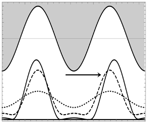
Figure 5(a) is a plot of the interface profile with time. This figure, drawn for the range  $0< x<2W$,
  $W$ being the half-width of the container, depicts two full waves for the wavy wall and two full waves for the initial interface perturbation. The corresponding maximum interface deflection,
  $h_{max}$, is plotted in figure 5(b). The markers in figure 5(b) denote the time corresponding to the interface profiles. Observe that the interface slides from left to right toward the wavy wall. Further, reminiscent of the flat wall, it is seen in figure 5(a) that the primary trough of the interface undergoes buckling to form secondary troughs in the vicinity of the top wall (cf. inset in figure 5a). This buckled configuration continues to evolve very slowly and in time exhibits sliding as a consequence of a symmetry-breaking instability wherein the interface translates parallel to the wall at
  $z=1$ (Lister et al. Reference Lister, Morrison and Rallison2006a; Glasner Reference Glasner2007; Lister, Rallison & Rees Reference Lister, Rallison and Rees2010; Dietze et al. Reference Dietze, Picardo and Narayanan2018). The necessary asymmetric perturbation that initiates the sliding motion in one direction or another is attributed to numerical truncation errors as mentioned by Dietze et al. (Reference Dietze, Picardo and Narayanan2018). The physical reason behind the sliding motion is associated with the dominance of capillary pressure gradients in the secondary troughs and to their surface curvature (Dietze et al. Reference Dietze, Picardo and Narayanan2018). The onset of sliding coincides with an increase of
  $h_{max}$ with time at around
  $t=1.5\times 10^{5}$. It is noteworthy that this sliding motion can be arrested by the presence of the wavy wall, depending on the amplitude of the wavy wall and the position of the interface (see movie 4 for the case of 1.5 cSt silicone oil in the main document and a similar movie for the case of 5 cSt silicone oil in the supplementary material). From our nonlinear simulations, we can determine this critical position of the interface for a given amplitude of the wavy wall, below which the sliding motion is hindered (cf. figure 6a). Above this critical value, the interface will always translate parallel to the wall at
  $z=1$ as shown in figure 6(b).

Figure 5. (a) Sliding of the interface as it approaches the wall:  $t=0$ (dotted),
  $t=1\times 10^{3}$ (dashed) and
  $t=1.5\times 10^{5}$ (solid). Here, the horizontal arrow points in the direction of sliding and the vertical arrow marks the direction in which gravity
  $(g)$ is acting on the fluids;
  $\mathcal {A}=0.4$ and
  $H_{1}=0.75$. (b) The temporal evolution of
  $h_{max}$. The markers denote the time corresponding to the interface profiles plotted in panel (a). Also see movie 4 for the evolution of the interface. The properties of water and silicone oil are
  $\rho _{1}=1000\,\textrm {kg}\,\textrm {m}^{-3}$,
  $\mu _{1}=1\times 10^{-3}\,\textrm {kg}\,\textrm {m}^{-1}\,\textrm {s}^{-1}$,
  $\rho _{2}=846\,\textrm {kg}\,\textrm {m}^{-3}$,
  $\mu _{2}=1.26\times 10^{-3}\,\textrm {kg}\,\textrm {m}^{-1}\,\textrm {s}^{-1}$ and
  $\gamma =0.0425\,\textrm {N}\,\textrm {m}^{-1}$.

Figure 6. (a) The critical position of the interface  $H_{1}/H$ for a given amplitude of the wavy wall
  $\mathcal {A}$. (b) Sliding of the interface as it approaches the wall:
  $t=0$ (dotted),
  $t=3\times 10^{5}$ (dashed) and
  $t=5\times 10^{5}$ (solid). Here, the horizontal arrow points in the direction of sliding and the vertical arrow marks the direction in which gravity
  $(g)$ is acting on the fluids;
  $\mathcal {A}=0.4$ and
  $H_{1}=0.85$. Also see movie 5 for the evolution of the interface.
4. Summary
Using a long-wavelength reduced-order model in conjunction with the WRIBL technique, it is shown that a deep patterned wall with periodic structure enhances the evolution of Rayleigh–Taylor instability of a thin film when the interface waveform is sub-harmonic to the shape of the wall – for example, when the interface has one full wave and the wall has two full waves. From the linear stability analysis a simple analytical expression for the growth rate is obtained for the case of a wavy wall with two full waves and an interface of one full wave. This expression shows the destabilizing effect of the wavy wall on the evolution of interfacial instability driven by gravity. In addition, nonlinear simulations for the case of a single fluid in contact with a passive gas show that the interface proceeds to rupture without sliding, whereas the bilayer system sandwiched by a wavy wall and a flat wall leads to the formation of troughs which slide due to symmetry-breaking of the solution. For a given amplitude of the wavy wall, a critical value of the position of the interface for the onset of the sliding motion is determined. Below this critical value the sliding motion is always arrested.
Supplementary material and movies
Supplementary material and movies are available at https://doi.org/10.1017/jfm.2021.960.
Funding
The authors gratefully acknowledge funding from NSF 2025117 and NASA via grant numbers NNX17AL27G and 80NSSC20M0093 (FSGC). T.C. acknowledges funding from the REU program, NSF EEC-1852111. Additionally, we thank an anonymous referee for several insightful comments.
Declaration of interests
The authors report no conflict of interest.


