


1. Introduction
Thin liquid films with fronts involving contact lines and their instabilities are relevant to applications in a number of different fields, ranging from nanoscale to macroscale films where instabilities are driven by a combination of various body forces, surface tension and wettability, see the reviews of Oron, Davis & Bankoff (Reference Oron, Davis and Bankoff1997) and Craster & Matar (Reference Craster and Matar2009). Significant progress has been reached by using a long-wave approximation, which simplifies considerably the analysis of thin film flows and their stability. In the context of thin films on a macroscale, the set-up involving a completely wetting film of constant thickness flowing down an incline has been understood reasonably well. For such a configuration, linear stability analysis (LSA) carried out in a moving reference frame leads to the dispersion relation, which shows stability for large wavenumbers, and predicts the most unstable wavelength (specifying the distance between emerging fingers), which results from the balance between destabilizing gravity and stabilizing surface tension forces (Troian et al. Reference Troian, Herbolzheimer, Safran and Joanny1989; Bertozzi & Brenner Reference Bertozzi and Brenner1997). However, as soon as some of the simplifying assumptions are removed, understanding the instability becomes much more complicated.
In the present paper, we focus on the funnel geometry, see figure 1, where initially a fixed amount of wetting fluid is deposited around a perimeter and then allowed to evolve due to gravity. Despite its relevance to a number of practical applications, funnel flow, to the best our knowledge, has not yet been carefully analysed, in particular in the context of front instabilities. Funnel flow involves geometry-induced convergence, and the influence of this convergence, as well as of azimuthal curvature on instability development, is unknown. For the purpose of understanding the stability properties of a film in a funnel, it is useful to discuss some of the many limiting configurations that could be related to that considered. If the film is deposited at a sufficient distance from the centre, the azimuthal curvature is small, and one could relate the problem to a finite volume of fluid deposited on an incline plane. Even that problem is, however, difficult to analyse due to a time-dependent base state (Goodwin & Homsy Reference Goodwin and Homsy1991; Gomba et al. Reference Gomba, Diez, Gratton, Gonzalez and Kondic2007). The limiting case of the opening angle  $\alpha = 90^{\circ }$ could be thought of as a flow down a cylinder (in a direction of the cylinder axis) (Smolka & SeGall Reference Smolka and SeGall2011; Mayo, McCue & Moroney Reference Mayo, McCue and Moroney2013), which shows fingering type of instabilities. Fingering instability is also observed for the flow down a surface of a cylinder or a sphere (Takagi & Huppert Reference Takagi and Huppert2010; Balestra et al. Reference Balestra, Badaoui, Ducimetière and Gallaire2019), a set-up which shows similarity to fingering observed during spin coating (Melo, Joanny & Fauve Reference Melo, Joanny and Fauve1989; Fraysse & Homsy Reference Fraysse and Homsy1994). Another set-up of interest is flow in a Hele–Shaw geometry where surface geometry plays a role in instability development (Miranda et al. Reference Miranda, Parisio, Moraes and Widom2000; Brandão, Fontana & Miranda Reference Brandão, Fontana and Miranda2014). In the limit
  $\alpha = 0^{\circ }$, one could think of the problem of closing a hole in a film on a horizontal substrate (Diez, Gratton & Gratton Reference Diez, Gratton and Gratton1992), which is stable (Backholm et al. Reference Backholm, Benzaquen, Salez, Raphaël and Dalnoki-Veress2014; Bostwick, Dijksman & Shearer Reference Bostwick, Dijksman and Shearer2017; Lv, Eigenbrod & Hardt Reference Lv, Eigenbrod and Hardt2018; Zheng et al. Reference Zheng, Fontelos, Shin, Dallaston, Tseluiko, Kalliadasis and Stone2018). Another possibly relevant limit is that of a liquid filament which, on a horizontal substrate, becomes unstable by a mechanism that could be related to the Rayleigh–Plateau instability of a liquid jet modified by the presence of a substrate (Davis Reference Davis1980). This problem is, however, difficult to analyse in the limit of zero contact angle that we consider here (Diez, González & Kondic Reference Diez, González and Kondic2009). Perhaps a closer analogy is a fluid ring on a horizontal substrate, which indeed may become unstable (Gonzalez, Diez & Kondic Reference Gonzalez, Diez and Kondic2013). However, the fact that there is no body force inducing converging flow makes this set-up significantly different from the funnel flow. The converging nature of the flow in a funnel leads to thickening of the film, and since the film thickness is important in determining both the speed of spreading and the instability mechanism itself, it is expected to influence the instability considerably. We should also point out that the problem opposite to our setting, a rising film in a glass, was considered recently (Dukler et al. Reference Dukler, Ji, Falcon and Bertozzi2020).

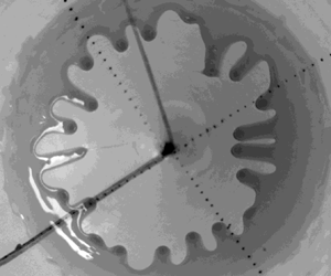
Figure 1. (a) Solidworks wire sketch of the  $47^{\circ }$ funnel. Note that the technical drawing mentions
  $45^{\circ }$; printing imperfections can somewhat modify the opening angle, which is therefore always measured after printing. (b) Photo of the experimental set-up including the latex sheet, stopper and green-light illumination. The beaker that collects the polydimethylsiloxane (PDMS) is visible underneath the funnel. Here,
  $S$ indicates the radius of the stopper used as initial barrier that releases the fluid. (c) Solidworks drawing of the
  $35^{\circ }$ funnel. (d) Coordinate system variables used in the description of the fluid behaviour (solid lines). The light-blue surface delineated with the dotted line indicates the initial fluid volume and position as created by the stopper at distance
  $r_{c0}$ (dotted arrow) from the origin of the funnel geometry; the thickness of the film referenced in the text,
  $h_i$, is measured in the vertical direction (therefore, along the short stopper dimension). The dashed arrow indicates the flow direction of the thin film. The arrow denoted by
  $g$ indicates the direction of gravity.
Various limiting cases suggest many possible routes for analysis of the instability evolution. In the present paper, we start by discussing our experimental results in § 2, and then follow in § 3 by considering appropriate models for describing spreading of a film on curved substrates. In § 4 we first discuss the generic features of the funnel flow, by discussing similarities and differences to the flow down an incline, with particular focus on the regime such that a useful input can be obtained by applying a self-similar approach. Then, in § 4.2 we apply the insights obtained in § 4.1 to interpret the experimental results, with particular focus on the instability development. Section 5 concludes the main part of the paper. LSA for a liquid film of constant flux flowing down an incline is briefly discussed in Appendix A. Supplementary materials available at https://doi.org/10.1017/jfm.2021.626 provide some technical details, experimental movies as well as the complete list of experimental results.
2. The experiment
We designed funnels with Solidworks and three-dimensional (3-D) printed them on a fused-deposition 3-D printer. Figure 1 shows the details of the funnels. Inside the funnel, we glued a thin latex sheet, which helped create a smoother surface. The funnel was placed between a green-light source and a beaker that collected the liquid flowing out of the funnel opening. To prepare the experiment, a 3-D printed stopper of radius  $S = 6\ \textrm {cm}$ was inserted in the funnel, see figure 1(b). A known volume of fluid,
  $V$, was then carefully deposited around the funnel using a syringe; the fluid spread itself evenly in the cavity around the stopper. This created an initial film of height
  $h_i$ (measured in the vertical direction), which we used as our control parameter to simplify interpretation of the results (note that
  $V \approx {\rm \pi}S h_i^{2}/\tan \alpha$). For every trial, the funnel and stopper were cleaned and levelled before deposition. For small values of the opening angle,
  $\alpha$, one needs a prohibitively large
  $V$ to keep
  $h_i$ in a range that is also appropriate for larger
  $\alpha$, so for such angles we chose smaller values of
  $h_i$. To start the flow, the stopper was raised and flow was observed. A fluorescent dye (pyrromethene) was added to the fluid stock solution, which enhanced the contrast between the moving fluid and the latex sheet under influence of the green light. We used PDMS of density
  $\rho = 9.6\times 10^{2}\ \textrm {kg}\ \textrm {m}^{-3}$, viscosity
  $\mu = 1\times 10^{3}\ \textrm {mPa}\ \textrm {s}$ and surface tension
  $\gamma = 21\ \textrm {mN}\ \textrm {m}^{-1}$; for more details regarding PDMS properties see Dijksman et al. (Reference Dijksman, Mukhopadhyay, Behringer and Witelski2019). Note that PDMS can be assumed to wet latex as the critical surface–vapour surface tension of typical latex types
  ${\sim}50\ \textrm {mJ}\ \textrm {m}^{-2}$ is much higher than the low surface tension of PDMS
  ${\sim}20\ \textrm {mJ}\ \textrm {m}^{-2}$ (Ho & Khew Reference Ho and Khew2000; Zhang et al. Reference Zhang, Vandaele, Seveno and De Coninck2018). This means that the spreading parameter is larger than 0 and thus the contact angle is zero, without hysteresis (see e.g. the book by De Gennes, Brochard-Wyart & Quéré Reference De Gennes, Brochard-Wyart and Quéré2004). Elastocapillary effects, such as discussed by Marchand et al. (Reference Marchand, Das, Snoeijer and Andreotti2012), were neglected as the ratio of liquid–vapour surface tension to elastic modulus of the latex rubber was much smaller than the thickness of the latex sheet
  ${\sim}1$ mm. Fluid flow was recorded using a high-resolution camera at 25 frames per second. The movies served both to extract the wavelength of the developing instability and for the quantitative assessment of the flow speeds of the relevant film features.
It should be pointed out that there were a few experimental issues that led to some variation in the extracted experimental results that are discussed later in the text (and denoted by error bars where appropriate). At first, the method to distribute the fluid, while simple, may not have always led to a perfect azimuthally symmetric distribution. Another source of error was the formation of air pockets under the thin rubber sheet lining the funnels. Re-gluing prior to conducting experiments helped to create a surface free of larger surface abnormalities. Conducting multiple experiments and averaging the values helped to remedy some of these errors and reduce the error bars. More detailed information regarding the experiments, including selected experimental movies (supplementary movies 1–4) as well as funnel specifications (Drawing 1, Drawing2) are available; additional movies can be found at the NJIT Capstone Laboratory web page (Kondic Reference Kondic2019).
2.1. Extracting instability features
The movies allowed us to extract two main features of the instability: the number of fingers observed,  $N_{exp}$, and the onset radius of fingering,
  $r_{c1}$. We show snapshots from the top-view movies for four values of
  $\alpha$ to identify such features in figure 2(a–d). The experiments for each set of parameters were repeated several times to obtain conclusive results, which are summarized in table 1, and shows
  $N_{exp}$, as observed for a few different values of
  $\alpha$ and
  $h_i$. We also carried out additional experiments using PDMS of lower viscosity,
  $\mu = 3.5\times 10^{2}\ \textrm {mPa}\ \textrm {s}$, which showed that
  $N_{exp}$ is viscosity-independent, a point to which we return in § 4.2. Before closing this section, we note that the rear contact line remained essentially fixed, with the fluid thinning in its vicinity, as can be seen clearly in the supplementary movies. This point will become relevant later when considering the self-similar solution.

Figure 2. (a–d) Flow examples for the  $60^{\circ }$,
  $47^{\circ }$,
  $35^{\circ }$ and
  $11^{\circ }$ opening angles, respectively. The width of each image is
  ${\sim}60\ \textrm {mm}$, as indicated by the dark circle that demarcates the edge of the fluid volume before onset of the flow. See also (a) supplementary movie 1; (b) supplementary movie 2; (c) supplementary movie 3; (d) supplementary movie 4.
Table 1. Experimental results for the flow in a funnel as the opening angle and the initial film thickness,  $h_i$, are varied (the latter is controlled via varying fluid volume,
  $V$). The columns are the funnel angle,
  $\alpha$, the initial fluid volume,
  $V$, the initial distance to the funnel centre,
  $r_{c0}$, the distance at which instability is observed,
  $r_{c1}$, the initial film height (in the
  $z$ direction),
  $h_i$, and the number of fingers observed,
  $N_{exp}$. Errors reported are standard deviations. If no standard deviation is reported, only one movie is available with a camera angle such that
  $r_{c1}$ could be extracted. Full datasets for experiments carried out also using PDMS of different viscosity, for additional fluid volumes and recorded using different camera angles are available, see supplementary table 1.

2.2. Extracting front speed
To determine the flow speed we need to extract quantitative data from the movies. In particular, we extracted the fingertip position as a function of time. First, we needed to know where  $r_{c1}$ was, the onset position of fingering. Figure 3(a) illustrates in more detail our approach to finding this value. We defined
  $r_{c1}$ by requiring that at the onset of fingering, the distinct undulations were present along the entire perimeter of the fluid front. We then needed to extract the fingertip position for each finger. To that end, we defined lines along the direction of motion of the fingers towards the funnel orifice. Figure 3(b) shows a few of these lines as an example. The lines are shown in red; they all converged in the funnel orifice. Along these lines, we extracted pixel values from the frames in the movies, which for every frame yielded an intensity profile as a function of
  $r$. Due to the dark front of the finger, every intensity profile had a clear step which could be fitted with an error function to obtain a fingertip position as a function of time. The intensity profiles extracted for every finger and every frame were put together to form a kymograph, which indicated qualitatively the fingertip dynamics for the tip considered. An example of such a kymograph is shown in figure 3(c). Note the linear part in the first few seconds of the kymograph, and the nonlinear slowing down for later times. Figure 3(d) zooms into the early times and confirms that the fingertip velocities were constant, and also that they depended on the opening angle,
  $\alpha$. This figure shows a few examples of the fingertip position as a function of time for three different values of
  $\alpha$. Tip positions were as measured from the finger starting point, which was always close to, but not exactly
  $r_{c1}$. Counterintuitively, the initial fingertip speed was larger for smaller
  $\alpha$, another point to which we will return in § 4.2.

Figure 3. (a) Front propagation as a function of time for the setting from figure 2. The middle part shows the onset of fingers, where they become countable and at which point we define  $r_{c1}$. (b) The dark front edge allows for fingertip position tracking along lines (red) of pixels towards the centre of the funnel (orifice). (c) A kymograph for the
  $60^{\circ }$,
  $h_i = 5$ mm case shows the tip position as a function of time. The initial part in the red square (duration of which is approximately 4 s) features an initially constant tip displacement rate. Examples of this initial fingertip position dynamics are shown in panel (d) for three different opening angles
  $60^{\circ }$,
  $47^{\circ }$ and
  $35^{\circ }$ for the same initial
  $h_i = 5\ \textrm {mm}$. Dash–dotted lines are straight lines as a guide to the eye to show the average tip speed for each value of
  $\alpha$. The time window shown in panel (d) corresponds approximately to the horizontal dimension of the red square in the kymograph shown in panel (c). Note the increase of the average speed with a decrease of
  $\alpha$, a point discussed further in § 4.2.
3. The model
In this section we discuss the appropriate model for a liquid film in a funnel. Consider a funnel of opening angle  $\alpha$, parametrized by
 \begin{equation} (x, y, z) = (r\cos\alpha\cos\theta, r\cos\alpha\sin\theta, r\sin\alpha), \quad r\in[R_l, R_r], \quad \theta\in[0, 2{\rm \pi}], \end{equation}
where  $0< R_l< R_r$. We can then define the orthogonal unit vectors on the funnel as
 \begin{equation} \left.\begin{gathered} \boldsymbol{e}_1 = (\cos\alpha\cos\theta, \cos\alpha\sin\theta, \sin\alpha),\quad \boldsymbol{e}_2 = (-\sin\theta, \cos\theta, 0), \\ \boldsymbol{n} = (-\sin\alpha\cos\theta, -\sin\alpha\sin\theta, \cos\alpha), \end{gathered}\right\} \end{equation}
where  $\boldsymbol {n}$ is the unit normal vector pointing inside the funnel, see figure 1(d). The principle normal curvatures in the directions parametrized by
  $r$ and
  $\theta$ are given by
  $\kappa _1 = 0, \kappa _2 = \tan \alpha /r.$ Based on the work of Roy, Roberts & Simpson (Reference Roy, Roberts and Simpson1997), the evolution of the thickness of a thin liquid film,
  $h$, inside a funnel can be described by the following partial differential equation:
 \begin{align} &\left(1 -
\frac{\tan\alpha}{r} \,h\right) h_t\nonumber\\
&\quad ={-}\frac{\gamma}{3\mu}\boldsymbol{\nabla}_s\boldsymbol{\cdot}\left[\left(h^{3}
- \frac{\tan\alpha}{2r}\,h^{4} \right)\boldsymbol{\nabla}_s
\left(\boldsymbol{\nabla}_s^{2} h + \frac{\tan\alpha}{r -
\tan\alpha h}\right) +
\frac{\tan^{2}\alpha\,h^{4}}{2r^{3}}\,\boldsymbol{e}_1\right]
\nonumber\\ & \qquad -\frac{\rho
g}{3\mu}\boldsymbol{\nabla}_s\boldsymbol{\cdot}\left[-\sin\alpha
h^{3}\left(1 - \frac{\tan\alpha}{r}
h\right)\boldsymbol{e}_1 - \cos\alpha
h^{3}\boldsymbol{\nabla}_s h \right],
\end{align}
\begin{align} &\left(1 -
\frac{\tan\alpha}{r} \,h\right) h_t\nonumber\\
&\quad ={-}\frac{\gamma}{3\mu}\boldsymbol{\nabla}_s\boldsymbol{\cdot}\left[\left(h^{3}
- \frac{\tan\alpha}{2r}\,h^{4} \right)\boldsymbol{\nabla}_s
\left(\boldsymbol{\nabla}_s^{2} h + \frac{\tan\alpha}{r -
\tan\alpha h}\right) +
\frac{\tan^{2}\alpha\,h^{4}}{2r^{3}}\,\boldsymbol{e}_1\right]
\nonumber\\ & \qquad -\frac{\rho
g}{3\mu}\boldsymbol{\nabla}_s\boldsymbol{\cdot}\left[-\sin\alpha
h^{3}\left(1 - \frac{\tan\alpha}{r}
h\right)\boldsymbol{e}_1 - \cos\alpha
h^{3}\boldsymbol{\nabla}_s h \right],
\end{align}
where surface gradient, divergence and Laplace operators are defined by
 \begin{equation} \left.\begin{gathered} \boldsymbol{\nabla}_s f = \frac{\partial f}{\partial r} \boldsymbol{e}_1 + \frac{1}{r\cos\alpha} \frac{\partial f}{\partial \theta} \boldsymbol{e}_2, \\ \boldsymbol{\nabla}_s \boldsymbol{\cdot} (q_1 \boldsymbol{e}_1 + q_2 \boldsymbol{e}_2) = \frac{1}{r}\, \frac{\partial}{\partial r} (r q_1) + \frac{1}{r\cos\alpha}\,\frac{\partial}{\partial \theta}(q_2),\\ \boldsymbol{\nabla}_s^{2} f = \frac{1}{r}\frac{\partial (r f_r)}{\partial r} + \frac{1}{r^{2}\cos^{2}\alpha} \frac{\partial^{2} f}{\partial \theta^{2}}, \end{gathered}\right\} \end{equation}
respectively. We non-dimensionalize the problem by  $h = a\, \bar {h}, r = a\, \bar {r}, t = t_c \, \bar {t},$ where
  $a=\sqrt {\gamma /\rho g}$ is the capillary length and
  $t_c = 3\mu a/ \gamma$ is the time scale. Howell (Reference Howell2003) pointed out that for a thin film such that
  $h \ll r/\tan (\alpha )$, the model can be simplified by neglecting asymptotically small terms; after dropping the bars, the governing equation is given by
 \begin{align} \frac{\partial h}{\partial t} \,{=}\,{-}\boldsymbol{\nabla}_s\boldsymbol{\cdot}\left\{h^{3}\left[\boldsymbol{\nabla}_s \left( \underbrace{\boldsymbol{\nabla}_s^{2} h}_\text{surface tension} + \underbrace{\frac{\tan\alpha}{r}}_\text{substrate curvature} \right)-\underbrace{\sin\alpha \boldsymbol{e}_1}_\text{tangential gravity} -\underbrace{\cos\alpha \boldsymbol{\nabla}_s h}_\text{normal gravity} \right]\right\}\!. \end{align}
For the experimental parameters given in § 2, we have  $a \approx 0.15$ cm and
  $t_c \approx 0.2$ s. For consistency with the experiment, we choose the computational domain
  $r\in [1, L]$,
  $L=100$,
  $\theta \in [0, 2{\rm \pi} ]$ and
  $h= O(1)$. The
  $r=1$ is chosen as the domain boundary so as to avoid the coordinate singularity at
  $r=0$.
The computational results that we discuss in § 4 are obtained by implementing second-order Crank–Nicolson method in time, second-order discretization in space and Newton's method to solve the nonlinear system at each time step, as described in detail by e.g. Lin & Kondic (Reference Lin and Kondic2010). To deal with the well-known issue of contact-line singularity, it is appropriate to introduce matched asymptotic expansions to join solutions in different length scales near the contact line, see Snoeijer & Andreotti (Reference Snoeijer and Andreotti2013) and Sibley, Nold & Kalliadasis (Reference Sibley, Nold and Kalliadasis2015) for further details. One can also introduce the interface potential that in general gives rise to an equilibrium film thickness. This film plays the role of a microscopic length scale that, again, has to be matched with an outer solution where viscous forces are not important (Pismen & Eggers Reference Pismen and Eggers2008). We, however, for simplicity assume directly that the solid substrate is prewetted, i.e. already covered by a thin layer of fluid. Assuming the presence of such a prewetted layer essentially removes the contact line from the consideration. While various other models including relaxation of no-slip boundary condition exist and could be implemented, it is known that from the macro-scale point of view (that is, consideration of the film dynamics) what really matters is the length scale that is introduced by a model (Diez, Kondic & Bertozzi Reference Diez, Kondic and Bertozzi2001). In particular, for a simple and well-researched constant flux flow down an incline (where a time-independent influx leading to a fixed film thickness far behind the front is assumed), it is known that there is a translationally invariant solution for a film moving down an incline with the speed  $U$ that only weakly depends on the precursor film thickness,
  $b_0$, as long as
  $b_0 \ll 1$ (Bertozzi & Brenner Reference Bertozzi and Brenner1997). It should be noted though that the limit
  $b_0\rightarrow 0$ is singular, which leads to a shock-like singularity; the details of the film behaviour in the presence of a vanishingly small length scale have been considered extensively in the literature, see e.g. Craster & Matar (Reference Craster and Matar2009) and Bonn et al. (Reference Bonn, Eggers, Indekeu, Meunier and Rolley2009); we do not discuss them further in the present work.
We note that while for a flow down an incline it can be assumed that the precursor film thickness is a constant (independent of position), for the flow in a funnel, conservation of fluid volume requires that the flux at the inlet and outlet are the same. One simple choice of the boundary conditions that satisfies this condition is
 \begin{align} h(r=1) = b_0\left(\frac{\dfrac{1}{L} + L\cos\alpha}{1 + \cos\alpha}\right)^{1/3},\quad h(L) = b_0, \quad \left.\boldsymbol{\nabla}_r\left(\boldsymbol{\nabla}_r^{2} h\right) - \cos\alpha \boldsymbol{\nabla}_r h\right|_{r=1, L} = 0. \end{align}
The precursor film thickness  $b(r)$ is obtained as the time-independent solution of the one-dimensional version of (3.5) (where the solution is assumed to be
  $\theta$-independent), and with the boundary conditions as specified by (3.6a–c). The solution of this nonlinear boundary value problem is found using Matlab's ‘fsolve’.
4. Results
In this section we present the results of analysis, simulations and comparison between theoretical predictions and experiments. In § 4.1 we focus on understanding the influence of funnel geometry on the flow without immediately attempting to develop direct comparison with the experiments. In this section we also discuss the insight that could be reached based on application of a self-similar type of approach. Then, in § 4.2 we focus on the comparison of the theoretical and the experimental results. As we will see, useful insight can be reached by developing a connection between the funnel flow and flow down an incline plane.
4.1. Film flow in a funnel: general considerations
4.1.1. Constant flux flow
For the incline plane flow, the best known case is the constant flux configuration and so we start by considering such a set-up in a funnel. The initial film profile specified at  $t=0$ is a (smoothed) rectangular profile of the unit height as follows:
 \begin{equation} h(r, t=0) = b(r) + \frac{1-b_0}{2}\left(1+\tanh(5(r-r_{c0}))\right), \end{equation}
where  $r_{c0}$ corresponds to the front position. Figure 4(a) shows the profiles that develop at different times. To better illustrate the influence of funnel geometry on the flow, we also show in panel (b) the results for constant flux flow down an incline. The latter results are obtained by solving numerically (A1) (see Appendix A), similar to those presented by e.g. Lin & Kondic (Reference Lin and Kondic2010), with a uniform precursor film,
  $b(r)\equiv b_0$, and consistent boundary conditions. Both sets of simulations show the formation of a capillary ridge behind the front, as expected. The comparison of the results for the flow in a funnel and down an incline shows that for the former, the film thickness is generally larger due to converging flow nature. Since the speed of the front is expected to scale with the film height as
  $U \propto h^{2}$ (Huppert Reference Huppert1982), this thickening also leads to a faster flow down a funnel compared with the flow down an incline, see figure 4(c). After initial transients, the latter evolves to a travelling wave moving with a constant speed, see figure 4(c,d). Within the presently used scaling, this speed is given by
  $U \sim h^{2} \sin \alpha$, see Appendix A and note that rescaled quantities are used there. The choice of relevant film thickness,
  $h$, entering this relation becomes more complicated for the constant volume flow, discussed in the following.

Figure 4. Constant flux flow: (a) funnel, azimuthally symmetric flow; (b) incline, unperturbed flow (for simplicity we use the same variable  $r$ for the both flows; in panel (b)
  $r$ stands for the downhill coordinate). The initial condition (dashed) for both (a,b) is specified by (4.1). The film profiles are shown at times
  $10$,
$10$,  $20$,
$20$,  $30$ and
  $40$ (solid lines). The speed (c) and the maximum height of the film (d) for the funnel flow (solid red) and for incline plane flow (dashed blue). The dotted (black) line in panel (c) shows the flow speed for a flow down an incline as discussed in the text; the difference between the computed and theoretical speed illustrates the (minor) influence of the initial transient behaviour. Here, the inclination angle is
  $\alpha = 60^{\circ }$, the initial front position is
  $r_{c0} = 80$ and
  $b_0 = 0.01$.
Before proceeding with a consideration of constant volume flow, we digress briefly to comment on the influence of precursor film thickness on the results. Figure 5 shows an example of the results obtained for  $b_0 = 0.005$,
  $0.01$ and
  $0.02$. We recall that for a film flowing down an incline plane in constant flux configuration, for larger precursor film thickness the spreading speed is (slightly) larger, see Appendix A. The same trend is found for the flow in a funnel, see figure 5(a,c). Figure 5(b) illustrates the steepening effect for the precursor film itself close to the funnel centre, at small values of
  $r$.
$r$.

Figure 5. Constant flux flow in a funnel: influence of the precursor film thickness for azimuthally symmetric flow. In all panels of the figure, the solid (blue), dashed (red) and dotted (black) lines correspond to  $b_0=0.005$,
  $0.01$ and
  $0.02$, respectively. (a) Film profiles at
  $t=45$, (b) precursor films, (c) speed of the spreading front and (d) maximum film height. Here
  $\alpha =60^{\circ }$ and
  $r_{c0}=80$.
4.1.2. Constant volume flow: self-similar approach
Next we study the spreading of a constant volume film in a funnel, focusing first on the insight that can be reached by considering the regimes where a self-similar solution can be formulated. For the flow down an incline, the self-similar solution (Huppert Reference Huppert1982) (ignoring surface tension effects) predicts that the front speed scales as  $t^{-2/3}$ and the height behind the ridge,
  $h_0$, as
  $t^{-1/3}$. The question is whether a similar approach could be used for the funnel flow.
Let us consider only the effect of substrate curvature and tangential gravity, and neglect all the other terms in (3.5). This simplification (valid sufficiently far behind the film front and for opening angles which are not too small) leads to
 \begin{equation} h_t = \frac{1}{r}\left[rh^{3}\left(\frac{\tan\alpha}{r^{2}}+\sin\alpha\right)\right]_r. \end{equation}
We observe that the substrate curvature amplifies the parallel component of gravity, and the amplification is larger when the flow is closer to the funnel centre. Next, we assume a solution of the form
 \begin{equation} h(r, t) = T(t)H(\eta), \quad \eta =\frac{R-r}{r_f(t)}, \end{equation}
where  $R$ specifies the position of the uphill part of the deposited fluid (assumed to be a constant, which is a good approximation of the experiment, as discussed in § 2),
  $r_f(t)$ is the distance travelled by the front and
  $R-r_f(t)$ is the position of the front, both at time
  $t$ (we drop the specific dependence on
  $t$ from now on). Equation (4.2) then leads to
 \begin{align} &\frac{\dot{T} r_f}{T \dot{r}_f} H - \eta H'\nonumber\\ &\quad = \frac{T^{2}}{\dot{r}_f} \left[ \frac{r_f}{R-r_f\eta} \left(\sin\alpha-\frac{\tan\alpha}{(R-r_f\eta)^{2}}\right) H^{3} - 3\left(\sin\alpha+\frac{\tan\alpha}{(R-r_f\eta)^{2}}\right)H^{2}H' \right], \end{align}
where the over-dot notation denotes the time derivative, and primes denote the derivative with respect to  $\eta$. The solution should satisfy the volume conservation condition
 \begin{equation} 2{\rm \pi}\int^{R}_{R - r_f(t)} r h(r, t)\,\textrm{d}r = 2{\rm \pi} T r_f\int^{1}_0 (R-r_f \eta)H(\eta)\,\textrm{d}\eta=v_c, \end{equation}
where  $v_c$ is the fluid volume.
At early times after fluid deposition,  $r_f\ll R$, and at the leading order in the small quantity
  $r_f/R$ we obtain
 \begin{equation} \frac{\dot{T} r_f}{T \dot{r}_f} H - \eta H' ={-}3c_s\frac{T^{2}}{\dot{r}_f}H^{2}H', \end{equation}
where  $c_s=\sin \alpha +\tan \alpha /R^{2}$, and the volume constraint at the leading order reads
 \begin{equation} T r_f\int^{1}_0 H(\eta)\,\textrm{d}\eta=\tilde{v}_{c}, \end{equation}
where  $\tilde {v}_{{c}}=v_c/(2{\rm \pi} R)$. We note that (4.6) and (4.7) are identical to those derived for the incline plane problem (Huppert Reference Huppert1982). Simple scaling arguments give
  $T(t)\sim t^{-1/3}$,
  $r_f(t)\sim t^{1/3}$ and therefore the self-similar solution is
 \begin{equation} h(r, t) = \frac{1}{\sqrt{3c_s}}\sqrt{\frac{R-r}{t}}. \end{equation}
The volume conservation constraint, (4.7), gives the location of the leading edge,
 \begin{equation} r_f(t) = \left(\frac{27c_s \tilde{v}_{c}^{2}}{4}\right)^{1/3} t^{1/3}, \end{equation}
and the film height at the front,
 \begin{equation} h(r=R-r_f, t) = \left(\frac{\tilde{v}_{c}}{2c_s}\right)^{1/3} t^{{-}1/3}. \end{equation}
This result shows that, in the limit when the fluid front only travels a short enough distance, the flow down a funnel is identical to the flow down an incline plane, a result which may not be immediately obvious.
4.1.3. Constant volume flow: convergence effects
To gain some insight into the influence of the convergent nature of the funnel flow, we use the self-similar solution specified by (4.8) as an ansatz (but one should keep in mind that this solution is only valid for  $r_f\ll R$) and require that the complete volume conservation constraint, (4.5), should be satisfied. Following this approach, we find that
  $r_f$ satisfies the following equation:
 \begin{equation} \frac{2R}{3}r_f^{3/2} - \frac{2}{5} r_f^{5/2} = \hat{c}\sqrt{t}, \end{equation}
where  $\hat {c}=\sqrt {3c_s}v_c/2{\rm \pi}$. By taking the time derivative, we obtain the equation for the front speed:
 \begin{equation} \frac{\textrm{d} r_f}{\textrm{d}t} = \frac{\hat{c}}{2(R r_f^{1/2} - r_f^{3/2})\sqrt{t}}. \end{equation}
Figure 6 shows the solution for the front position ( $R-r_f$) and the front speed (
 $\textrm {d}r_f/\textrm {d}t$). We see that the convergence effect leads to acceleration of the front at later times. To analyse this acceleration in more detail, we note that for the later stage of spreading, when the front is close to the funnel centre, we may assume
  $R - r_f\ll R$. For the discussion of this regime, it is convenient to introduce the stopping time
  $T_s = (4/(15 \hat {c}))^{2}\, R^{5}$, at which the fluid front reaches the funnel centre,
  $r_f (T_s) = R$. We can then rewrite (4.11) as
 \begin{equation} \frac{2}{3}\left(1 - \frac{R-r_f}{R}\right)^{3/2} - \frac{2}{5} \left(1 - \frac{R-r_f}{R}\right)^{5/2} = \frac{4}{15}\sqrt{1 - \frac{T_s-t}{T_s}}. \end{equation}
At the leading order in the small quantity  $(R-r_f)/R$, we obtain
  $R-r_f =\sqrt {{4R^{2}}/{15 T_s}} \,\sqrt {T_s - t}$. Therefore, the front speed
  $\dot {r}_f$ scales as
  $(T_s-t)^{-1/2}$ showing that the front is expected to accelerate when approaching the funnel centre.

Figure 6. Constant volume flow in a funnel: predictions based on self-similar approach. (a) Front position ( $R-r_f$), (b) front speed (
 $\textrm {d}r_f/\textrm {d}t$) in (4.11) and (4.12) (note log–log scale in panel (b)). Here
  $R=90$ and
  $\hat {c}=1370$, corresponding to the same funnel angle and volume used later in figure 7.
4.1.4. Constant volume flow: numerical solution
Next, we study the spreading of a constant volume film in a funnel utilizing numerical simulations. The initial film profile at  $t=0$ is specified by the following expression:
 \begin{equation} h(r, t=0) = b(r) + \frac{1-b_0}{2}\left(\tanh(5(r-r_{c0})) + \tanh(5(r_{c0}+w-r))\right), \end{equation}
where  $r_{c0}$ corresponds to the front position and
  $w$ determines the fluid volume. Figure 7 shows the film profiles, both for (a) funnel geometry and (b) for the same fluid volume travelling down an incline plane. For the flow down an incline, we observe film thinning, as expected. For the funnel flow, we observe different behaviour, with the thinning effect significantly reduced or even inverted for the later times. As a consequence, the film in a funnel spreads significantly faster.

Figure 7. Constant volume flow: (a) funnel, azimuthally symmetric flow; (b) incline, unperturbed flow. The initial condition (dashed) is the same for (a,b) and is specified by (4.14). The film profiles are shown at times  $50$,
$50$,  $100$,
  $150$,
  $200$ and
  $250$ (solid lines). The speed (c) and the maximum height of the film (d) for the funnel flow (solid red) and incline plane flow (dashed blue) (note log–log scale). The dotted (black) lines in (c,d) plot the self-similar solutions (4.9)–(4.10), respectively; note that (4.10) applies to the thickness behind the capillary ridge, leading to an approximately constant offset to the numerical solution for the maximum height. Slight deviation of the numerical solution from the expected scaling for very early times illustrate the minor influence of the initial transient behaviour. Here, the inclination angle is
  $\alpha = 60^{\circ }$, the initial front position is
  $r_{c0} = 80$,
  $w=10$ and
  $b_0 = 0.01$.
Figure 7(c,d) show that the scaling laws predicted by the self-similar solution (Huppert Reference Huppert1982) are accurately reproduced for the constant volume flow down an incline. Regarding the front speed shown in figure 7(c) and ignoring transient effects for very early times, the self-similar solution specified by (4.9) captures precisely its behaviour for early times, including the prefactor. Regarding figure 7(d), note that here we plot numerical result for the maximum film height, not the height behind the ridge to which the similarity solution applies; however, since the behaviour of the two considered quantities is essentially the same, the power law expected from the self-similar solution, (4.10), captures well the behaviour of the maximum height for early times of the evolution, modulo an (constant) offset.
Focusing next on the funnel flow, we note the speed-up of the fluid front for the late times, as predicted by the self-similar solution derived in § 4.1.2. This speed-up is not as strong as predicted (viz. figure 6b), which is not surprising since the self-similar approach is not expected to be accurate for late times. Figure 7(d) also shows the corresponding increase of the film height. This thickening effect, which is also relevant for the intermediate times shown in figure 7, is responsible for the deviation from the spreading law predicted by the self-similar solution (note deviation of the slope of the red lines in figure 7(c,d) from the scaling expected by the self-similar solution for the flow down an incline).
Figure 8 shows the results obtained for the constant volume flow in the funnel geometry as the opening angle,  $\alpha$, is varied. The film spreads faster down a funnel characterized by larger
  $\alpha$, as shown in panel (a). We suspect that the tangential gravity may have a dominant effect on the time scale of the flow; to show that this is the case, we plot the results for the front position and maximum film height versus
  $t\sin \alpha$ in panels (b and c). We find approximate collapse of the front position curves in the panel (b), which shows that indeed the tangential gravity plays the major role. Regarding the maximum film height shown in panel (c), we observe that this quantity is larger for larger
  $\alpha$, as expected since the capillary ridge is more pronounced for such angles (we expect that this effect is also responsible for slightly faster spreading for larger
  $\alpha$ observed in panel (b)). However, the trend of the maximum heights is similar for all
  $\alpha$, with the film height decreasing for early times, while at the later times when the front reaches closer to the funnel centre, the film height increases, see panel (c), and faster spreading is observed, see panel (b).

Figure 8. Funnel flow: constant fluid volume spreading as the opening angle  $\alpha$ is varied. (a) Film profiles at
  $t=250$. The initial conditions are taken to be the same, shown by the dashed line. The position of the spreading front and the maximum film height are shown in (b,c), respectively (note log–log scale in (c)). Here, the initial front position is
  $r_{c0} = 80$,
  $w=10$ and
  $b_0 = 0.01$.
4.1.5. Instability development
To obtain a basic idea regarding instability development (finger formation), we discuss first the flow down an incline plane for the constant flux configuration. In such a set-up, the base state (for which the film thickness does not depend on the transverse coordinate), translates down an incline at a constant speed  $U$, as already discussed. This fact allows for carrying out the linear stability analysis in the moving frame translating (with speed
  $U$) with the film itself; in this frame the base state is time-independent (Bertozzi & Brenner Reference Bertozzi and Brenner1997). Appendix A briefly outlines this problem, and discusses in particular the wavenumber of maximum growth,
  $q_m$, the corresponding wavelength,
  $\lambda _m = {2 {\rm \pi}/q_m}$, as well as the critical wavenumber
  $q_c$, such that the wavenumbers
  $q> q_c$ are stable; see figure 12 in Appendix A. The stability analysis becomes more complicated for the constant volume flow down an incline (Gomba et al. Reference Gomba, Diez, Gratton, Gonzalez and Kondic2007), since for that problem the base state itself is evolving, as also illustrated in figure 7(b). For the flow in a funnel, viz. figure 7(a), an additional complication involves the gradual thickening of the film due to convergent flow.
In § 4.2 we will consider a rather simple approach to utilize the LSA results in the incline plane problem for a comparison with experiment; here we outline the basic aspect of this approach, without explicit reference to the experiment. Let us consider constant volume flow in a funnel, as shown in figure 9. When the film front has reached a prescribed position for the considered opening angle,  $\alpha$, the thickness
  $h_0$ is extracted from the film profile as the thickness at the inflection point behind the capillary ridge. With the knowledge of this characteristic thickness,
  $h_0$, and the opening angle,
  $\alpha$, we can then find a travelling wave solution on an incline plane that has the exact same characteristic thickness; such a solution is plotted in figure 9 as well (marked by P). The LSA results of this travelling wave solution then give us the most unstable wavenumber. Therefore, this most unstable wavenumber results from a combination of the information from experiments (instability location), numerical simulations of funnel flow (providing
  $h_0$) and the LSA originating from the flow down an inline plane. In the next section, we discuss how to use a similar approach to provide a basic understanding of the instability development in experiment.

Figure 9. Film profiles in a funnel (‘F’, constant volume) and on an incline plane (‘P’, constant flux). The former is the film profile at  $t=50$ in figure 7(a). The latter is a travelling wave solution with the film thickness behind the front corresponding to the thickness at the inclination point of ‘F’. This thickness,
  $h_0$, determines the scale that is used in the LSA.
4.2. Film flow in a funnel: comparison with the experiment
We now proceed to the consideration of a funnel flow, but with a specific emphasis on the comparison with the experiments. While we will modify the choice of the parameters that we use to more closely resemble the experimentally relevant ones, for simplicity we still keep the smoothed rectangular initial profile, with the idea that the instability takes some time to develop, and therefore the initial film profile is not of relevance. However, we do choose the initial film width,  $w$, see (4.14), so as to be consistent with the experimental fluid volume (in units of
  $a^{3}$) by
  $V = 2 {\rm \pi}S h_0 w$, with
  $S$ in units of
  $a$ and
  $h_0 = 1$. We note that the choice that has been made in selecting the parameters (in particular, having fixed film thickness and varying fluid volume as the opening angle
  $\alpha$ is modified) simplifies the connection to the experiments; the price to pay is the increased complexity of the results, in particular when discussing the trends of the results as
  $\alpha$ is modified, as we will see in the following.
Figure 10 shows the results for both funnel simulations (denoted F) and for the same fluid volume travelling down an incline plane (denoted P), for the fluid volumes corresponding to the experimental ones. When comparing the thicknesses of the capillary ridge between funnel and incline plane flow, the effects related to the convergent nature of the funnel flow become relevant, as discussed in § 4.1.4. In particular, when considering the change of the capillary ridge thickness as the opening angle  $\alpha$ is varied, we need to remember that in the simulations the volume increases as
  $\alpha$ decreases from
  $60^{\circ }$ to
  $45^{\circ }$ and
  $30^{\circ }$ (to keep approximate consistency with the experiments), which leads to thicker films and ridges. Since we are interested more in the trends than in exactly matching theory with experiments, we keep round numbers for the angles that we use, because the differences in the results are minor. The influence of the volume increase is visible in figure 10, where we observe a non-monotonous dependence of the capillary ridge thickness on
  $\alpha$.

Figure 10. Time evolution of a film on an incline plane (P) and in a funnel (F). The initial condition is specified by (4.14). The results are plotted at the times at which the experimentally observed instability radius,  $r_{c1}$, is reached. Note that the shown range of
  $r$,
$r$,  $40$, is the same for all figure panels. The initial volume corresponds to that experimentally used for the film height of 5 mm for
  $\alpha = 60^{\circ }$,
  $47^{\circ }$ and
  $35^{\circ }$, and of 2.5 mm for
  $\alpha = 11^{\circ }$, see table 1.
Next we proceed with application of LSA to the present problem. To make progress, we choose an approach that allows us to reach a basic understanding of the instability development observed in the experiments. LSA, as already discussed, is based on the incline plane problem and the constant flux set-up, using the film thickness behind the capillary ridge,  $h_0$, as the appropriate scale, see figure 9. We assume that the film is initially deposited at
  $r= r_{c0}$, so that the fluid volume forms a circle of radius
  $r_{c0}\cos \alpha$. As the film flows down a funnel, the radius of this circle,
  $r_c(t)$, becomes smaller, and the film itself thins (for the chosen initial condition). To make a comparison with experiments, we choose the characteristic thicknesses,
  $h_0$, as the thickness obtained from simulations at the time when the film front reaches
  $r_{c1}$, where the onset of fingering extracted from the experimental results occurs, as illustrated in figure 10. Table 2 lists the values of
  $h_0 (r_{c1})$ for a few values of
  $\alpha$ and for the widths
  $w$ of the initial condition that lead to the experimental fluid volumes. Additional simulations (not shown for brevity) show that
  $h_0 (r_{c1})$ is essentially the same for any reasonable choice of the initial fluid geometry.
Table 2. Results and predictions of the linear stability analysis for the experimental fluid volumes. The initial film thickness  $h_0 (r_{c0}) = 1.0$. The columns are as follows:
  $\alpha$ – the funnel opening angle, similar to the experimental values, see table 1;
  $w$ – the width of the initial condition in time-dependent simulations as used in figure 10;
  $r_{c1}$ – the position at which instability is observed in the experiments;
  $h_0$ at
  $r_{c1}$ – as obtained in the simulations for funnel flow, see the text for details;
  $q_m$ – the most unstable wavenumber obtained by LSA;
  $q_c$ – critical wavenumber obtained by LSA;
  $\lambda _m = {2 {\rm \pi}/q_m}$;
  $N_{LSA}$ – prediction for the number of fingers based on
  $\lambda _m$ and
  $r_{c1}$. The values used for
  $r_{c0}$ (initial front position) and those from the experiments are listed in table 1; note that the listed values of
  $w$ combined with the specified values of
  $r_{c0}$ and
  $h_0 (r_{c0})$ lead to the same fluid volume as in the experiments.

Figure 11 plots the obtained results for the most unstable wavelength predicted by LSA together with the experimentally measured one; the LSA results are also shown in table 2. The experimental wavelength is defined by  $\lambda = 2{\rm \pi} \cos (\alpha )r_{c}/N_{exp}$, and is given in units of the capillary length. We note that it is crucial to use the film thickness
  $h_0(r_{c1})$ when comparing the predictions of the LSA and experiment: using the initial film thickness does not lead to a meaningful agreement. The number of fingers predicted by LSA,
  $N_{LSA}$ (given also in table 2), can be compared directly with the values obtained in the experiments,
  $N_{exp}$, see table 1. We find that the agreement is excellent for larger opening angles, however for small angles the most unstable wavelength found by LSA is larger than that by experiment. There is a number of possible reasons for this difference, which include an increased influence of the azimuthal curvature that is not included in the presented methodology (note that
  $r_{c1}$ is smaller for small
  $\alpha$), or simply the fact that slow development of instability for small values of
  $\alpha$ may involve additional effects, such as a transient growth mechanism which was proposed for the flow down an incline (Bertozzi & Brenner Reference Bertozzi and Brenner1997).

Figure 11. Funnel: average finger spacing wavelength,  $\lambda$, versus opening angle,
  $\alpha$, including experiments (Exp, filled green symbols) for which
  $r_{c1}$ is available (see table 1), as well as matching linear stability analysis (LSA, open black symbols) predictions from table 2. For completeness we plot the results for all available values of
  $h_i$ per angle. Symbols indicate
  $h_i$:
  $\square$ –
  $h_i = 5$ mm for
  $60^{\circ }$,
  $47^{\circ }$,
  $35^{\circ }$, and
  $h_i = 2.5$ mm for
  $11^{\circ }$;
  ${\triangle}$ –
  $h_i = 7$ mm for
  $60^{\circ }$;
  $\triangleleft$ –
  $h_i = 7$ mm for
  $47^{\circ }$;
  $\triangleright$ –
  $h_i = 3$ mm for
  $11^{\circ }$;
  $\diamond$ –
  $h_i = 4$ mm for
  $11^{\circ }$.
Next, we proceed with an explanation (at least in qualitative terms) of some perhaps counterintuitive trends from the experimental results. Figure 3(d) shows an increase of the finger tip speed as the opening angle is decreased. Measuring the typical slopes in this figure, we find that finger tip speed increases by the factors of (approximately)  $1.5$ and
  $2.5$ as the opening angle decreases from
  $\alpha = 60^{\circ }$ to
  $47^{\circ }$ and
  $35^{\circ }$, respectively. Recalling now the expected scaling for the front speed,
  $U \approx h_0^{2} \sin \alpha$, and using the values for
  $h_0$ at the instability onset from table 2, we find that this expression for
  $U$ provides a good approximation for the front tip speed (the corresponding ratios are approximately 1.8 and 2.2). Therefore, an increase of the value of
  $h_0$ as the opening angle decreases has a stronger influence then a decrease of
  $\sin (\alpha )$. One should keep in mind of course that the above expression for
  $U$ applies to an unperturbed front while the experimental results from figure 3 are obtained by measuring the tip speed, and therefore only an approximate agreement could be expected.
To explain the increase of the typical instability wavelength as  $\alpha$ is decreased, recall that based on the standard scaling argument, the (dimensional) most unstable wavelength scales with the film thickness behind the front,
  $h_0$, see Appendix A. Note that this scaling argument is only approximate, since based on the LSA for the constant flux flow down an incline, see figure 12 in Appendix A, the inclination angle influences the most unstable wavelength as well. Still, the scaling
  $\lambda _m \propto h_0 (r_{c1})$ appears to be a good description of the experimental results, as can be seen from tables 1 and 2.

Figure 12. Results of LSA for a liquid film on an incline plane with different  $D$. The precursor film thickness is
  $b_0=0.01$.
4.2.1. Discussion
Reasonable agreement between theory and experiments, in particular for larger opening angles, shows that our approach combining the information from experiments, simulations and LSA describes well the main features of instability development. Before closing this section, we list a few additional comments and observations.
(i) The reader may wonder whether simply using
 $h_i$ from the experiments (see table 1) could be done to describe the instability development and emerging length scales. This approach however does not lead to a reasonable estimate, since there is a considerable change in the film thickness between $r_{c0}$ and $r_{c1}$. One may also wonder whether the results of LSA may depend on the initial condition in simulations (which is chosen ad hoc): the answer is again no, since the film does not develop instability immediately; by the time $r_{c1}$ is reached, the memory of the initial condition is lost.
(ii) There are two main differences between the flow down an incline and in a funnel: one is film thickening due to the convergent nature of the flow, as discussed in §§ 4.1.2 and 4.1.4; the other is the presence of azimuthal curvature for the funnel flow, which we have not discussed in much detail. The curvature in the azimuthal direction scales as
$1/r$, see § 3, so it is a small quantity as long as only large values of $r$ are considered. This value should be compared with the typical curvature (in the radial direction) of the film itself, which is an $O(1)$ quantity close to the film front. Smallness of the azimuthal curvature justifies ignoring it in the present work, since it is expected to become important only very close to the funnel centre. Therefore, as long as the fluid front is far away from the centre, the flow in a funnel is similar to the flow down an incline plane, as long as the fact that the film thickens due to volume conservation is taken into account.(iii) Figure 10 specifies the times at which instability starts to develop (when the fluid front reaches
$r_{c1}$). We note that these times are shorter for the funnel compared with flow down an incline, in particular for smaller $\alpha$; this is due to the film thickening for the flow in a funnel. Thicker films flow faster and also become unstable sooner, compared with the flow down an incline.(iv) In light of the discussion in this section, the experimental fact that the observed number of fingers does not depend on fluid viscosity (see supplementary table 1) may not be obvious. While viscosity only changes the time scale of the flow, for the present problem the time scale may be important since the film thickness changes with time. However, the location at which the film becomes unstable,
$r_{c1}$, and the film thickness behind the capillary ridge, $h_0$, turn out not to depend on the fluid viscosity, which supports the presented approach for carrying out LSA and the interpretation of the results.(v) LSA predicts that instability will develop if the circumference
$2{\rm \pi} r_{c}\cos \alpha$ is larger than $\lambda _c = {2 {\rm \pi}/q_c}$. Consistently, the maximum number of unstable modes (leading to fingers in experiments) that can be supported is $\lfloor {2{\rm \pi} r_{c}\cos \alpha /\lambda _c}\rfloor$, where $\lfloor {\cdot }\rfloor$ is the floor function. One untested consequence of this result is that if the film is released close to the centre of the funnel, it may not become unstable since the circumference of the circle formed by the initial fluid front may not be long enough to support instability development.


5. Conclusions
The presented results show that a reasonably complete understanding of the instability development for a film flowing in a funnel can be reached by combining the insight from experiments and asymptotic analysis to allow for a significant simplification of the governing equations. Furthermore, it turns out that despite the complexity of the problem, useful insight can be also reached by considering a self-similar approach similar to that used for the flow down an incline plane. Such insight from self-similar methods combined with LSA originating from the flow down an incline provides important guidance in carrying out numerical simulations that help to develop a better understanding of the instability development. While we have focused on a particular geometry of flow in a funnel, we note that a similar approach could be applied to a number of other unstable flows, such as the flows on a sphere, on the outside surface of a funnel or even in more complicated geometries.
To conclude, we note that instabilities of the systems whose base state evolves in time are difficult to analyse in a tractable manner. For the present problem, we have shown that reasonably good insight can be reached by simplifying the problem first, and then using some input regarding instability development from the experiments. One would of course like to be able to understand the general features of instability development, including the factors that govern instability onset itself. Reaching this goal will require further development of stability analysis and is left as an open problem for future work.
Supplementary material and movies
Supplementary material and movies are available at https://doi.org/10.1017/jfm.2021.626, which includes movies of selected experiments, technical drawings of one of the funnels used for experiments and the Excel data sheet including the results of additional experiments.
Acknowledgements
We thank V. Saggiomo for help with 3-D printing of the funnels, and to the undergraduate students E. Figueroa, J. Parchment and Y. Xu (supervised by R. Allaire, PhD candidate at the time when experiments were carried out) for help with the experiments and data analysis as a part of their Capstone class at NJIT.
Funding
This work was supported by Ministry of Science and Technology, Taiwan (T.S.L., grant number MOST-109-2115-M-009-006-MY2) and by the National Science Foundation, USA (L.K., grant numbers CBET-1604351 and DMS-1815613).
Declaration of interests
The authors report no conflict of interest.
Note added in proof
It came to our attention during the review process that a similar topic was discussed in a recent paper (Xue & Stone Reference Xue and Stone2021), to which the reader is directed for complementary results.
Appendix A. Stability of the constant flux flow down an incline plane
Consider a completely wetting fluid flowing down a planar surface enclosing an angle  $\alpha$ with the horizontal. With the same scales as used in the main body of the paper, the evolution equation of the film thickness can be written as (see e.g. Bertozzi & Brenner Reference Bertozzi and Brenner1997; Kondic Reference Kondic2003)
 \begin{equation} \frac{\partial}{\partial t} h ={-}\boldsymbol{\nabla}\boldsymbol{\cdot}[h^{3}\nabla^{3} h - \cos\alpha h^{3}\boldsymbol{\nabla} h +\sin\alpha h^{3} \boldsymbol{e}_x], \end{equation}
where  $\boldsymbol {e}_x$ is the unit vector pointing in the positive
  $x$-direction. Re-normalizing the variables as
  $h = h_0 \bar {h}$,
  $t = \bar {t}/{ (h_0^{5} \sin ^{4}\alpha )^{1/3}}$,
  $x = ({h_0/\sin \alpha })^{1/3} \bar {x}$, one obtains the well-known model of a thin liquid film (after dropping the bars),
 \begin{equation} \frac{\partial}{\partial t} h ={-}\boldsymbol{\nabla}\boldsymbol{\cdot}[h^{3}\nabla^{3} h - D h^{3}\boldsymbol{\nabla} h +h^{3} \boldsymbol{e}_x], \end{equation}
where  $D= (h_0/\sin \alpha )^{2/3}\cos \alpha$. This equation admits a one-dimensional travelling wave solution that satisfies
 \begin{equation} -Uh + h^{3}h_{xxx} - D h^{3}h_x + h^{3}=c, \end{equation}
where boundary conditions  $h(x=\infty )=b_0$,
  $h(x=-\infty )=1$ are imposed to have
  $U = 1+b_0+b_0^{2}$,
  $c = -(b_0+b_0^{2}).$ (Note that the (unscaled) speed of the front scales with the film thickness squared, as can be seen from the ratio of the scaling factors for
  $x$ and
  $t$.) Linear stability of the film with respect to perturbations in the transverse,
  $y$, direction is conveniently carried out in a moving coordinate frame,
  $s = x - Ut$, where we assume the solution of the form
 \begin{equation} h(s, y, t) = H(s) + \epsilon g(s)\textrm{e}^{\sigma t} \textrm{e}^{\textrm{i}q y}, \end{equation}
where  $H(s)$ satisfies (A3). At
  $O(\epsilon )$ we obtain a linear eigenvalue problem for
  $g(s; q)$ with eigenvalue
  $\sigma$ that represents the growth rate of the temporal evolution of the perturbation at each wave number. Figure 12 shows the results of this analysis; for more details see e.g. Kondic (Reference Kondic2003).


