2 Effective constitutive equations for non-dilute viscoelastic particle suspensions

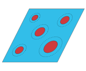
Figure 1. Representative volume element (RVE) of the microstructure. Subjected to a macroscopic velocity gradient $\bar{\boldsymbol{L}}$, the microstructure will begin to evolve through a sequence of configurations from its initial state (a) at time $t=0$ into its deformed configuration (b) at $t=t_{0}$. We consider solid Kelvin–Voigt (KV) particles (red ellipses) suspended in a Newtonian matrix fluid (blue). On average, the particles deform into general ellipsoids, whose shape and orientation with respect to the laboratory axes $\{\boldsymbol{E}_{k}\}_{k=1}^{3}$ are characterized by the ratios of their semi-axes $w_{1}=z_{2}/z_{1}$, $w_{2}=z_{3}/z_{1}$ and the orthonormal triad $\{\boldsymbol{n}_{k}\}_{k=1}^{3}$ (all of which evolve with the deformation), as shown in (c). The larger dotted ellipses surrounding the particles illustrate the ellipsoidal symmetry of the two-point probability function of the particle distribution.

In this work we make use of the constitutive model of Avazmohammadi & Ponte Castañeda (Reference Avazmohammadi and Ponte Castañeda2015) for dispersions of neutrally buoyant deformable particles suspended in a Newtonian matrix fluid under Stokes flow conditions ($\mathit{Re}\ll 1$). The model will be used here to investigate the oscillatory shear rheology of non-dilute suspensions of initially spherical viscoelastic particles. The suspending fluid has viscosity $\unicode[STIX]{x1D702}^{(1)}$, while the particles are assumed to have Kelvin–Voigt (KV) constitutive behaviour with linear viscosity given by $\unicode[STIX]{x1D702}^{(2)}$ and nonlinear elastic response described by the Gent (Reference Gent1996) model, which, in turn, is characterized by the ground-state shear modulus $\unicode[STIX]{x1D707}$ and strain-locking parameter $J_{m}$, as described in more detail further below. The particles are randomly distributed in volume fraction $c$, as illustrated in figures 1(a) and 1(b) depicting respectively ‘snapshots’ of a representative volume element (RVE) of the suspension at the initial time and at a later time. As shown in figure 1(a), the particles are initially spherical in their unstressed state. We note that more general initial shapes could be considered for the particles; however, in this work the focus shall be on suspensions of initially spherical viscoelastic particles. Upon loading, the particles deform and the microstructure evolves through a time-dependent sequence of configurations in which the particles become aligned ellipsoids of identical (on average) evolving shape and orientation, as depicted in figure 1(b). The larger dotted ellipses around the particles illustrate the ellipsoidal symmetry of their two-point probability functions (Ponte Castañeda & Willis Reference Ponte Castañeda and Willis1995), which, for simplicity, are assumed here to have the same ‘shape’ and ‘orientation’ as the particles. Thus, we identify as microstructural variables the particle aspect ratios

(2.1a,b)$$\begin{eqnarray}w_{1}=z_{2}/z_{1},\quad w_{2}=z_{3}/z_{1},\end{eqnarray}$$

along with the orthonormal triad $\{\boldsymbol{n}_{k}\}_{k=1}^{3}$ characterizing the orientation of the semi-axes of the particles with respect to the laboratory reference frame $\{\boldsymbol{E}_{k}\}_{k=1}^{3}$, as depicted in figure 1(c). In the above equations, $z_{1}$, $z_{2}$ and $z_{3}$ quantify the lengths of the semi-axes of the ellipsoidal particles.

Before providing the detailed equations describing the homogenization model of Avazmohammadi & Ponte Castañeda (Reference Avazmohammadi and Ponte Castañeda2015) for the above-described suspensions, it is useful to recall that the model provides a generalization for non-dilute concentrations of viscoelastic particles of the results of Gao et al. (Reference Gao, Hu and Ponte Castañeda2011) for dilute suspensions of elastic particles. As such, the model is exact for dilute particle concentrations, but should still provide reasonably accurate estimates for low-to-moderate particle volume fractions. As discussed in the introduction and in more detail in the above-mentioned references, this is a consequence of the use of a generalization of the Hashin–Shtrikman variational estimates of Ponte Castañeda & Willis (Reference Ponte Castañeda and Willis1995) for elastic composites consisting of random distributions of aligned particles of ellipsoidal shape with ellipsoidal distribution for the particle centres, together with the reinterpretation of Kailasam & Ponte Castañeda (Reference Kailasam and Ponte Castañeda1998) for linearly viscous composites with evolving microstructure. The model is not meant to be used for large volume fractions of mono-disperse particles, because it cannot accurately capture strong interactions of particles in close vicinity. However, as will be seen below, even for dilute suspensions, changes in the shape and orientation of the particles affect the instantaneous macroscopic viscosity and normal stress differences to the same order as the particle volume fraction – and, as a consequence, large volume fractions are not required to generate strongly nonlinear rheological effects.

According to the model of Avazmohammadi & Ponte Castañeda (Reference Avazmohammadi and Ponte Castañeda2015), the macroscopic Cauchy stress tensor is given by

(2.2)$$\begin{eqnarray}\displaystyle \bar{\unicode[STIX]{x1D748}}=-\bar{p}\unicode[STIX]{x1D644}+\bar{\unicode[STIX]{x1D749}}, & & \displaystyle\end{eqnarray}$$

where the arbitrary pressure $\bar{p}$ is the Lagrange multiplier associated with the incompressibility constraint $\text{tr}\,\bar{\unicode[STIX]{x1D63F}}=0$, and the extra-stress tensor is given by

(2.3)$$\begin{eqnarray}\displaystyle \bar{\unicode[STIX]{x1D749}}=(1-c)\bar{\unicode[STIX]{x1D749}}^{(1)}+c\bar{\unicode[STIX]{x1D749}}^{(2)}=(1-c)\bar{\unicode[STIX]{x1D749}}^{(1)}+c(\bar{\unicode[STIX]{x1D749}}_{e}^{(2)}+\bar{\unicode[STIX]{x1D749}}_{v}^{(2)}), & & \displaystyle\end{eqnarray}$$

in terms of the average viscous stresses in the Newtonian matrix and the particle phase, $\bar{\unicode[STIX]{x1D749}}^{(1)}$ and $\bar{\unicode[STIX]{x1D749}}_{v}^{(2)}$, as well as the average elastic stress in the particle phase $\bar{\unicode[STIX]{x1D749}}_{e}^{(2)}$. Making use of the constitutive equation for the viscous stress in the particle, this can be rewritten in the form

(2.4)$$\begin{eqnarray}\displaystyle \bar{\unicode[STIX]{x1D749}}=2\unicode[STIX]{x1D702}^{(1)}\bar{\unicode[STIX]{x1D63F}}+2c(\unicode[STIX]{x1D702}^{(1)}-\unicode[STIX]{x1D702}^{(2)})\bar{\unicode[STIX]{x1D63F}}^{(2)}+c\bar{\unicode[STIX]{x1D749}}_{e}^{(2)}, & & \displaystyle\end{eqnarray}$$

where it is noted that $\bar{\unicode[STIX]{x1D749}}$ need not be deviatoric in general. The effective rate-of-strain tensor will be denoted by $\bar{\unicode[STIX]{x1D63F}}$ and is the symmetric part of the macroscopic velocity gradient $\bar{\boldsymbol{L}}$. In the above equation, $\bar{\unicode[STIX]{x1D63F}}^{(2)}$ is the average strain-rate tensor in the particle phase given by

(2.5)$$\begin{eqnarray}\displaystyle \bar{\unicode[STIX]{x1D63F}}^{(2)}=\{\mathbb{I}-2(1-c)(\unicode[STIX]{x1D702}^{(1)}-\unicode[STIX]{x1D702}^{(2)})\mathbb{P}\}^{-1}\{\bar{\unicode[STIX]{x1D63F}}-(1-c)\mathbb{P}\bar{\unicode[STIX]{x1D749}}_{e}^{(2)}\}, & & \displaystyle\end{eqnarray}$$

where $\mathbb{I}$ is the fourth-order identity tensor with minor and major symmetry. The tensor $\mathbb{P}$ is a fourth-order microstructural tensor that depends on the particle aspect ratios, $w_{1}$ and $w_{2}$. Expressions for the Cartesian coordinates of $\mathbb{P}$ for ellipsoidal particles in a Newtonian host fluid are given in appendix A.

As already mentioned, the elastic response of the KV particles is described by the Gent model, which provides a relation between the extra stress in the particles and the deformation gradient and depends on two material parameters: the ground-state shear modulus $\unicode[STIX]{x1D707}$ and the strain-locking parameter $J_{m}$. The Gent model provides a generalization of the classical neo-Hookean (NH) finite-strain model, where $J_{m}$ is used to describe the strong stiffening of elastomers as the macromolecular chains become elongated with the deformation. The limit as $J_{m}\rightarrow \infty$ corresponds to neo-Hookean behaviour, which does not exhibit strain locking at any finite strain. As discussed in some detail in § 2.1 of Avazmohammadi & Ponte Castañeda (Reference Avazmohammadi and Ponte Castañeda2015), the Gent model leads to the following evolution equation for the extra elastic stress in the particles:

(2.6)$$\begin{eqnarray}\displaystyle \stackrel{\!\!\!\!\!\!\triangledown }{\bar{\unicode[STIX]{x1D749}}_{e}^{(2)}}=2\unicode[STIX]{x1D707}\bar{\unicode[STIX]{x1D63F}}^{(2)}+\frac{2}{\unicode[STIX]{x1D707}J_{m}}\text{tr}[\bar{\unicode[STIX]{x1D63F}}^{(2)}(\bar{\unicode[STIX]{x1D749}}_{e}^{(2)}+\unicode[STIX]{x1D707}\unicode[STIX]{x1D644})](\bar{\unicode[STIX]{x1D749}}_{e}^{(2)}+\unicode[STIX]{x1D707}\unicode[STIX]{x1D644}). & & \displaystyle\end{eqnarray}$$

Here $\stackrel{\!\!\!\!\!\!\triangledown }{\bar{\unicode[STIX]{x1D749}}_{e}^{(2)}}$ is the upper-convected time derivative of the average extra elastic stress over the particles. In the limit $J_{m}\rightarrow \infty$, (2.6) reduces to the known rate form of the neo-Hookean model (Joseph Reference Joseph1990).

Evolution of microstructure. The evolution of the aspect ratios characterizing the average shape of the particles is given by

(2.7)$$\begin{eqnarray}\displaystyle & \displaystyle \frac{\text{d}w_{1}}{\text{d}t}=w_{1}(\boldsymbol{n}_{2}\boldsymbol{\cdot }\bar{\unicode[STIX]{x1D63F}}^{(2)}\boldsymbol{n}_{2}-\boldsymbol{n}_{1}\boldsymbol{\cdot }\bar{\unicode[STIX]{x1D63F}}^{(2)}\boldsymbol{n}_{1}), & \displaystyle\end{eqnarray}$$

(2.8)$$\begin{eqnarray}\displaystyle & \displaystyle \frac{\text{d}w_{2}}{\text{d}t}=w_{2}(\boldsymbol{n}_{3}\boldsymbol{\cdot }\bar{\unicode[STIX]{x1D63F}}^{(2)}\boldsymbol{n}_{3}-\boldsymbol{n}_{1}\boldsymbol{\cdot }\bar{\unicode[STIX]{x1D63F}}^{(2)}\boldsymbol{n}_{1}), & \displaystyle\end{eqnarray}$$

where $\bar{\unicode[STIX]{x1D63F}}^{(2)}$ is the average strain-rate tensor in the particle phase given in (2.5). The orthonormal vectors $\{\boldsymbol{n}_{k}\}$ characterize the average orientation of the particle semi-axes. Their evolution is governed by

(2.9)$$\begin{eqnarray}\displaystyle \dot{\boldsymbol{n}}_{k}=\unicode[STIX]{x1D734}\boldsymbol{n}_{k}, & & \displaystyle\end{eqnarray}$$

where the particle or microstructural spin tensor has Cartesian components with respect to the triad $\{\boldsymbol{n}_{k}\}$ given by

(2.10)$$\begin{eqnarray}\displaystyle \unicode[STIX]{x1D6FA}_{ij}=\bar{W}_{ij}^{(2)}-\frac{(w_{i-1})^{2}+(w_{j-1})^{2}}{(w_{i-1})^{2}-(w_{j-1})^{2}}\bar{D}_{ij}^{(2)}\quad \forall i\neq j, & & \displaystyle\end{eqnarray}$$

with $w_{1-1}=w_{0}=1$. In addition, $\bar{W}_{ij}^{(2)}$ are the Cartesian components of the average vorticity tensor in the particle phase given by

(2.11)$$\begin{eqnarray}\displaystyle \bar{\unicode[STIX]{x1D652}}^{(2)}=\bar{\unicode[STIX]{x1D652}}+(1-c)\mathbb{R}[2(\unicode[STIX]{x1D702}^{(1)}-\unicode[STIX]{x1D702}^{(2)})\bar{\unicode[STIX]{x1D63F}}^{(2)}-\bar{\unicode[STIX]{x1D749}}_{e}^{(2)}], & & \displaystyle\end{eqnarray}$$

where $\bar{\unicode[STIX]{x1D652}}$ is the macroscopic vorticity tensor and the Cartesian components of the microstructural tensor $\mathbb{R}$ are given in appendix A as functions of the particle aspect ratios $w_{1}$ and $w_{2}$. It should be noted that these evolution laws generalize corresponding expressions (e.g. Goddard & Miller Reference Goddard and Miller1967; Wetzel & Tucker Reference Wetzel and Tucker2001) for dilute suspensions. Due to the hypotheses implicit in its derivation via variational estimates of the Hashin–Shtrikman–Willis type, the above constitutive model is expected to be most appropriate for polydisperse systems, although it should also hold for monodisperse systems up to moderate particle concentrations (Ponte Castañeda & Willis Reference Ponte Castañeda and Willis1995).

Simple shear. Subsequently, we subject suspensions of initially spherical viscoelastic particles $(w_{1}|_{t=0}=w_{2}|_{t=0}=1)$ to simple shear excitations. Then, prescribing a strain-rate excitation $\dot{\unicode[STIX]{x1D6FE}}(t)$, the macroscopic velocity gradient in simple shear can be written as

(2.12)$$\begin{eqnarray}\displaystyle \bar{\boldsymbol{L}}=\dot{\unicode[STIX]{x1D6FE}}(t)\boldsymbol{E}_{1}\boldsymbol{E}_{2}. & & \displaystyle\end{eqnarray}$$

The particles will deform and assume the shape of general ellipsoids characterized – on average – by the aspect ratios $w_{1}$ and $w_{2}$. In simple shear, the particles rotate only in the $\boldsymbol{E}_{1}$–$\boldsymbol{E}_{2}$ plane of shearing, such that their orientation may be described in terms of a single angle $\unicode[STIX]{x1D703}$ and (2.9) reduces to

(2.13)$$\begin{eqnarray}\displaystyle \dot{\unicode[STIX]{x1D703}}=\boldsymbol{n}_{\mathbf{2}}\boldsymbol{\cdot }\unicode[STIX]{x1D734}\boldsymbol{n}_{\mathbf{1}}=-\bar{W}_{12}^{(2)}+\frac{1+w_{1}^{2}}{1-w_{1}^{2}}\bar{D}_{12}^{(2)}. & & \displaystyle\end{eqnarray}$$

We wish to study the behaviour of the suspensions of viscoelastic particles under harmonic strain excitations of the form

(2.14)$$\begin{eqnarray}\displaystyle \unicode[STIX]{x1D6FE}(t)=\unicode[STIX]{x1D6FE}_{0}\sin (\unicode[STIX]{x1D714}t), & & \displaystyle\end{eqnarray}$$

where $\unicode[STIX]{x1D6FE}_{0}$ is the amplitude of the strains and $\unicode[STIX]{x1D714}$ is the angular excitation frequency. Consequently, the strain rate is given by

(2.15a,b)$$\begin{eqnarray}\dot{\unicode[STIX]{x1D6FE}}(t)=\dot{\unicode[STIX]{x1D6FE}}_{0}\cos (\unicode[STIX]{x1D714}t),\quad \dot{\unicode[STIX]{x1D6FE}}_{0}=\unicode[STIX]{x1D6FE}_{0}\unicode[STIX]{x1D714}.\end{eqnarray}$$

In order to conveniently discuss the results, we introduce the dimensionless parameters

(2.16a,b)$$\begin{eqnarray}K=\frac{\unicode[STIX]{x1D702}^{(2)}}{\unicode[STIX]{x1D702}^{(1)}},\quad G=\frac{\unicode[STIX]{x1D702}^{(1)}\dot{\unicode[STIX]{x1D6FE}}_{0}}{\unicode[STIX]{x1D707}},\end{eqnarray}$$

as proposed by Avazmohammadi & Ponte Castañeda (Reference Avazmohammadi and Ponte Castañeda2015). Additionally, we define the dimensionless excitation frequency

(2.17)$$\begin{eqnarray}\displaystyle F=\frac{\unicode[STIX]{x1D702}^{(1)}\unicode[STIX]{x1D714}}{\unicode[STIX]{x1D707}}, & & \displaystyle\end{eqnarray}$$

which is a ratio between the intrinsic time scale $\unicode[STIX]{x1D702}^{(1)}/\unicode[STIX]{x1D707}$ and the process time scale $\unicode[STIX]{x1D714}^{-1}$.

Thus, for oscillatory simple shear loading conditions, the constitutive model requires the time integration of (2.7), (2.8) and (2.13) for the particle aspect ratios $w_{1}$ and $w_{2}$ and orientation angle $\unicode[STIX]{x1D703}$, together with (2.6) for the Cartesian components of particle average elastic stress $\bar{\unicode[STIX]{x1D749}}_{e}^{(2)}$. These equations are solved numerically using an explicit fourth-order Runge–Kutta time-integration scheme. The solutions in the time-periodic steady state were obtained by time-walking the system through at least ten loading cycles until the limit orbits were attained. In this connection, it is noted that the limit cycles are fairly insensitive to the initial conditions. The numerical integration for obtaining the components of the microstructural tensor $\mathbb{P}$ were carried out using a Gauss–Legendre quadrature.

In the context of the above-mentioned equations for simple shear loading conditions, it is also relevant to recall that a linear stability analysis carried out for dilute concentrations of NH elastic particles (of initially spherical shape) showed that the steady-state solution under constant shear rate is stable (Gao, Hu & Ponte Castañeda Reference Gao, Hu and Ponte Castañeda2012). In addition, recent numerical simulations of the time-dependent response of such soft particle systems (Villone & Maffettone Reference Villone and Maffettone2019) have confirmed the analytical solutions (Gao et al. Reference Gao, Hu and Ponte Castañeda2012) and not shown any indication of the possible development of instabilities. This may suggest that the solutions of the above system of equations for simple shear loading under more general oscillatory conditions will also be stable, provided that the particles are initially spherical (and that the suspending fluid is Newtonian). However, this remains to be investigated further. On the other hand, it should be noted that Gao et al. (Reference Gao, Hu and Ponte Castañeda2012) found that, depending on the initial particle shape and dimensionless parameter $G$, three types of long-time solutions are possible for suspensions of initially non-spherical NH particles subjected to constant shear rate: tank-treading, tumbling and trembling – with an interesting bifurcation phenomenon from the trembling to the tumbling solution.

3 Small amplitude oscillatory shear (SAOS)

To put our results for LAOS into context, we begin by exploring the rheological properties of moderately concentrated suspensions of initially spherical viscoelastic particles under small amplitude oscillatory shear (SAOS). For small strains and initially spherical particles in simple shear, the constitutive equations presented in the previous section can be shown to reduce to the Oldroyd equations

(3.1)$$\begin{eqnarray}\displaystyle \bar{\unicode[STIX]{x1D749}}+\unicode[STIX]{x1D706}_{1}\dot{\bar{\unicode[STIX]{x1D749}}}=2\unicode[STIX]{x1D702}_{0}(\bar{\unicode[STIX]{x1D63F}}+\unicode[STIX]{x1D706}_{2}\dot{\bar{\unicode[STIX]{x1D63F}}}), & & \displaystyle\end{eqnarray}$$

with an effective viscosity

(3.2)$$\begin{eqnarray}\displaystyle \unicode[STIX]{x1D702}_{0}=\frac{2+3c}{2(1-c)}\unicode[STIX]{x1D702}^{(1)}, & & \displaystyle\end{eqnarray}$$

and where the two macroscopic time scales $\unicode[STIX]{x1D706}_{1}$ and $\unicode[STIX]{x1D706}_{2}$ can be identified as

(3.3a,b)$$\begin{eqnarray}\unicode[STIX]{x1D706}_{1}=\frac{3+2c}{2(1-c)}\frac{\unicode[STIX]{x1D702}^{(1)}}{\unicode[STIX]{x1D707}}+\frac{\unicode[STIX]{x1D702}^{(2)}}{\unicode[STIX]{x1D707}},\quad \unicode[STIX]{x1D706}_{2}=\frac{3(1-c)}{2+3c}\frac{\unicode[STIX]{x1D702}^{(1)}}{\unicode[STIX]{x1D707}}+\frac{\unicode[STIX]{x1D702}^{(2)}}{\unicode[STIX]{x1D707}}.\end{eqnarray}$$

In obtaining (3.1), use was made of the fact that the constitutive equations for NH solids are the small-strain limit of the Gent model (2.6) for reasonable values of $J_{m}$. It can be shown (see appendix B) that the above equations reduce to the constitutive equations of the Newtonian solvent phase and to the linear small-strain viscoelasticity model for the KV particle phase, respectively, in the limits $c\rightarrow 0$ and $c\rightarrow 1$. Furthermore, equation (3.2) for $\unicode[STIX]{x1D702}_{0}$ recovers the well-known Einstein result in the dilute limit.

Figure 2. Storage and loss moduli normalized by the shear modulus $\unicode[STIX]{x1D707}$ as functions of the dimensionless frequency $F=\unicode[STIX]{x1D702}^{(1)}\unicode[STIX]{x1D714}/\unicode[STIX]{x1D707}$ in the SAOS regime. (a) $G^{\prime }/\unicode[STIX]{x1D707}$ and $G^{\prime \prime }/\unicode[STIX]{x1D707}$ for suspensions of NH particles ($K=0.0$) at different particle volume fractions $c$. (b) $G^{\prime }/\unicode[STIX]{x1D707}$ and $G^{\prime \prime }/\unicode[STIX]{x1D707}$ for suspension with 20 vol.% KV particles for different viscosity ratios $K$.

After an initial transient phase under harmonic loading such as (2.14), the suspension will reach a dynamic steady state in which the shear stress component $\bar{\unicode[STIX]{x1D70F}}_{12}$ can be written as

(3.4)$$\begin{eqnarray}\displaystyle \bar{\unicode[STIX]{x1D70F}}_{12}(t)=\unicode[STIX]{x1D6FE}_{0}G^{\prime }\sin (\unicode[STIX]{x1D714}t)+\unicode[STIX]{x1D6FE}_{0}G^{\prime \prime }\cos (\unicode[STIX]{x1D714}t), & & \displaystyle\end{eqnarray}$$

where $G^{\prime }$ and $G^{\prime \prime }$ are the storage and loss moduli, respectively. By substituting the above ansatz for $\bar{\unicode[STIX]{x1D70F}}_{12}$ into (3.1), we obtain the expressions

(3.5a,b)$$\begin{eqnarray}G^{\prime }=\frac{(\unicode[STIX]{x1D706}_{1}-\unicode[STIX]{x1D706}_{2})\unicode[STIX]{x1D702}_{0}\unicode[STIX]{x1D714}^{2}}{1+\unicode[STIX]{x1D706}_{1}^{2}\unicode[STIX]{x1D714}^{2}},\quad G^{\prime \prime }=\frac{(1+\unicode[STIX]{x1D706}_{1}\unicode[STIX]{x1D706}_{2}\unicode[STIX]{x1D714}^{2})\unicode[STIX]{x1D702}_{0}\unicode[STIX]{x1D714}}{1+\unicode[STIX]{x1D706}_{1}^{2}\unicode[STIX]{x1D714}^{2}},\end{eqnarray}$$

as functions of the excitation frequency $\unicode[STIX]{x1D714}$. We recall that in the above equations the two macroscopic time scales $\unicode[STIX]{x1D706}_{1}$ and $\unicode[STIX]{x1D706}_{2}$, as well as the effective viscosity $\unicode[STIX]{x1D702}_{0}$, are functions of the mechanical properties of the constituents and the particle volume fraction. In the dilute limit, a Taylor series expansion of (3.5) about $c=0$ recovers the first-order correction terms for the dynamic rigidity and the dynamic viscosity given in equations (69) and (70) in Roscoe (Reference Roscoe1967). In the limit $\unicode[STIX]{x1D714}\rightarrow 0$, the viscous stresses in the solvent phase do not suffice to elastically deform the particles, so that $G^{\prime }\rightarrow 0$ as $\unicode[STIX]{x1D714}\rightarrow 0$, while the dynamic state viscosity $G^{\prime \prime }/\unicode[STIX]{x1D714}\rightarrow \unicode[STIX]{x1D702}_{0}$. In the high-frequency limit, the storage modulus plateaus at

(3.6)$$\begin{eqnarray}\displaystyle \lim _{\unicode[STIX]{x1D714}\rightarrow \infty }G^{\prime }=(\unicode[STIX]{x1D706}_{1}-\unicode[STIX]{x1D706}_{2})\unicode[STIX]{x1D702}_{0}/\unicode[STIX]{x1D706}_{1}^{2}, & & \displaystyle\end{eqnarray}$$

while the dynamic viscosity is given by

(3.7)$$\begin{eqnarray}\displaystyle \lim _{\unicode[STIX]{x1D714}\rightarrow \infty }G^{\prime \prime }/\unicode[STIX]{x1D714}=\unicode[STIX]{x1D706}_{2}\unicode[STIX]{x1D702}_{0}/\unicode[STIX]{x1D706}_{1}. & & \displaystyle\end{eqnarray}$$

Figure 2(a) shows two small-strain frequency sweeps of storage and loss moduli for suspensions of purely elastic particles with different particle volume fractions $c$. We see that as $c$ increases from 10 vol.% to 30 vol.%, the loss modulus decreases and the storage modulus increases. The suspension becomes less dissipative and the macroscopic response appears more solid-like for larger particle volume fractions. Figure 2(b) shows storage and loss moduli as functions of the excitation frequency for suspensions with 20 vol.% KV particles and different viscosity ratios $K$. For higher values of $K$, the overall small-strain response of the suspension becomes more dissipative and less elastic, as expected.

Figure 3. Storage and loss moduli as a function of the excitation frequency $\unicode[STIX]{x1D714}$ for a suspension of purely elastic ($K=0.0$) particles at high volume fractions. (a) For $c=c_{cr}\approx 0.41$, the curves for $G^{\prime }$ and $G^{\prime \prime }$ just intersect at one frequency $\unicode[STIX]{x1D714}=\unicode[STIX]{x1D714}_{cr}$. (b) For $c=0.6$, $G^{\prime }>G^{\prime \prime }$ for a finite range of frequencies $\unicode[STIX]{x1D714}_{1}<\unicode[STIX]{x1D714}<\unicode[STIX]{x1D714}_{2}$.

Figure 3 shows the behaviour of $G^{\prime }$ and $G^{\prime \prime }$ for a suspension of purely elastic particles ($K=0.0$) at larger particle concentrations. In particular, figure 3(a) shows that, for sufficiently large concentrations ($c=c_{cr}$), the curves for $G^{\prime }$ and $G^{\prime \prime }$ just intersect at a critical frequency $\unicode[STIX]{x1D714}=\unicode[STIX]{x1D714}_{cr}$, while figure 3(b) shows that, for $c>c_{cr}$, there is a range of frequencies for which $G^{\prime }>G^{\prime \prime }$, indicating a predominantly solid-like behaviour for the suspension. To determine conditions for the existence of intersection points for $G^{\prime }$ and $G^{\prime \prime }$ more precisely, we use (3.5) and set $G^{\prime }|_{\unicode[STIX]{x1D714}=\unicode[STIX]{x1D714}_{1/2}}=G^{\prime \prime }|_{\unicode[STIX]{x1D714}=\unicode[STIX]{x1D714}_{1/2}}$. Solving for $\unicode[STIX]{x1D714}_{1/2}$, we find two roots

(3.8)$$\begin{eqnarray}\displaystyle \unicode[STIX]{x1D714}_{1/2}=\frac{1}{2\unicode[STIX]{x1D706}_{1}\unicode[STIX]{x1D706}_{2}}(\unicode[STIX]{x1D706}_{1}-\unicode[STIX]{x1D706}_{2}\mp \sqrt{(\unicode[STIX]{x1D706}_{1}-\unicode[STIX]{x1D706}_{2})^{2}-4\unicode[STIX]{x1D706}_{1}\unicode[STIX]{x1D706}_{2}}), & & \displaystyle\end{eqnarray}$$

suggesting that storage and loss moduli can intersect if the inequality $(\unicode[STIX]{x1D706}_{1}-\unicode[STIX]{x1D706}_{2})^{2}-4\unicode[STIX]{x1D706}_{1}\unicode[STIX]{x1D706}_{2}\geqslant 0$ is satisfied. Using (3.3), the above inequality may be rewritten as

(3.9)$$\begin{eqnarray}\displaystyle \left[\frac{3+2c}{2(1-c)}-\frac{3(1-c)}{2+3c}\right]^{2}-4\left[\frac{3+2c}{2(1-c)}+K\right]\left[\frac{3(1-c)}{2+3c}+K\right]\geqslant 0, & & \displaystyle\end{eqnarray}$$

which can be seen to be dependent on the particle volume fraction $c$ as well as the ratio between particle and solvent viscosity $K$. We conclude that there is a frequency range, $\unicode[STIX]{x1D714}_{1}\leqslant \unicode[STIX]{x1D714}\leqslant \unicode[STIX]{x1D714}_{2}$, for which $G^{\prime }\geqslant G^{\prime \prime }$, such that the small-strain response of the suspension is predominantly solid-like. As seen in figure 3 for suspensions of purely elastic particles ($K=0.0$), the model predicts a solid-like region for particle volume fractions $c\geqslant c_{cr}=0.40721$.

Figure 4. Shear stress normalized by shear modulus $\unicode[STIX]{x1D707}$ for suspensions with 20 vol.% purely elastic particles under SAOS at $\unicode[STIX]{x1D6FE}_{0}=0.05$ and $F=1.0$. (a) Normalized shear stress $\bar{\unicode[STIX]{x1D70F}}_{12}/\unicode[STIX]{x1D707}$ as a function of dimensionless time $\unicode[STIX]{x1D702}^{(1)}\unicode[STIX]{x1D714}/\unicode[STIX]{x1D707}$. (b) Normalized shear stress $\bar{\unicode[STIX]{x1D70F}}_{12}/\unicode[STIX]{x1D707}$ in the stress–strain-rate space at small excitation amplitude $\unicode[STIX]{x1D6FE}_{0}=0.05$.

Figure 4(a) shows the stress response as a function of time $t$ for a suspension with 20 vol.% purely elastic particles in the SAOS regime. The stress waveform is sinusoidal and shifted in phase with respect to the excitation $\unicode[STIX]{x1D6FE}$. In the phase space $\bar{\unicode[STIX]{x1D70F}}_{12}$ versus $\dot{\unicode[STIX]{x1D6FE}}$, the sinusoidal stress waveform is an ellipse as can be seen in figure 4(b). The stress waveform and the limit cycle shown in figure 4 are characteristic of linear material responses. Normal stress differences are not observed in the small-strain regime.

At this point, it should also be noted that, given a soft particle suspension, experimentally obtained SAOS sweeps could be used to determine some of the model parameters, provided that we can measure accurately at least one of them. As we have seen, the SAOS response, as determined by expressions (3.5) for $G^{\prime }$ and $G^{\prime \prime }$, is a function of the fluid viscosity, the particle viscosity and elasticity, as well as the particle volume fraction. Therefore, using the asymptotic expressions for $G^{\prime }$ and $G^{\prime \prime }$ as $\unicode[STIX]{x1D714}$ approaches 0 and $\infty$, three equations could be generated for the four parameters. For example, if the easy-to-measure fluid viscosity is known, the volume fraction, elasticity and viscosity of the particles could be determined.

4 Large amplitude oscillatory shear (LAOS)

As we transition into the regime of large-strain amplitudes, the evolution of the microstructure gives rise to a number of nonlinear features as well as anisotropic behaviour. In this section we want to provide a detailed study of the nonlinearities that characterize the macroscopic large-strain behaviour of non-dilute dispersions of highly deformable particles.

Figure 5. Amplitude sweep for storage and loss moduli for suspensions with 20 vol.% purely elastic particles ($K=0.0$) under oscillatory simple shear at frequency $F=1.0$. (a) Storage modulus $G^{\prime }$ normalized by $\unicode[STIX]{x1D707}$ for suspensions of NH and Gent particles. (b) Loss modulus $G^{\prime \prime }$ normalized by $\unicode[STIX]{x1D707}$ for suspensions of NH and Gent particles.

Figures 5(a) and 5(b) show $G^{\prime }$ and $G^{\prime \prime }$, respectively, as functions of the strain amplitude for suspensions of purely elastic particles ($K=0.0$). Results are given for suspensions of Gent particles with strain-locking behaviour characterized by $J_{m}=10$ and dispersions of NH particles with no strain locking characterized by $J_{m}\rightarrow \infty$. For sufficiently large-strain amplitudes $\unicode[STIX]{x1D6FE}_{0}$, figure 5 reveals that the storage and loss moduli become general functions of the strain amplitude $\unicode[STIX]{x1D6FE}_{0}$, in addition to the excitation frequency $\unicode[STIX]{x1D714}$. Since the small-strain limit of the Gent model (2.6) is identical to the NH model, $G^{\prime }$ and $G^{\prime \prime }$ are independent of the strain-locking parameter in the small amplitude regime ($\unicode[STIX]{x1D6FE}_{0}<0.3$). However, as we move into the large amplitude regime, figure 5 shows that, for suspensions of NH particles ($J_{m}\rightarrow \infty$), both storage and loss moduli monotonically decrease. On the other hand, for suspensions of Gent particles ($J_{m}=10.0$), figure 5(b) reveals that $G^{\prime \prime }$ assumes a local maximum at $\unicode[STIX]{x1D6FE}_{0}\approx 3.0$.

Based on the above observations and in accordance with the terminology of Hyun et al. (Reference Hyun, Kim, Ahn and Lee2002), we can identify the suspensions of NH particles as ‘type I’ (strain thinning) fluids, characterized by monotonically decreasing $G^{\prime }$ and $G^{\prime \prime }$ at the transition into the nonlinear regime, while we classify the dispersions of Gent particles as ‘type III’ (weak strain overshoot) fluids, characterized by the local maximum that $G^{\prime \prime }$ assumes near $\unicode[STIX]{x1D6FE}_{0}=3.0$. Furthermore, it is useful to recall (Hyun et al. Reference Hyun, Kim, Ahn and Lee2002) that type I fluids typically exhibit shear-thinning behaviour, as a result of the microstructure aligning itself in the direction of flow, which is consistent with the predictions of the model of Avazmohammadi & Ponte Castañeda (Reference Avazmohammadi and Ponte Castañeda2015) for suspensions of NH particles under steady shear and sufficiently large-strain rates $\dot{\unicode[STIX]{x1D6FE}}$; in fact, the model predicts that effective steady-state viscosity may even drop below the solvent viscosity $\unicode[STIX]{x1D702}^{(1)}$. On the other hand, the local maximum in $G^{\prime \prime }$ appears to coincide with the occurrence of a peak in the distorted stress waveform for suspensions of Gent particles (as will be discussed later), which suggests that the observed type III behaviour is due to the strain locking of the Gent particles at the larger strain amplitudes.

For large-strain amplitudes, the storage and loss moduli do not suffice to describe the rheological behaviour of the suspensions of interest here. Higher-order Fourier coefficients must be considered in order to provide a complete picture of the mechanical response. However, instead of discussing the higher-order Fourier coefficients, we proceed to examine the characteristic stress waveforms, as well as the elastic and viscous projections of the so-called Lissajous–Bowditch curve for suspensions of highly deformable particles in the LAOS regime. The various stress waveforms and limit cycles were obtained by numerically evolving the system through at least ten loading cycles in order to erase all memory of the initial conditions. In this context, it should be noted that the limit cycles were found to be insensitive to the initial conditions.

Figure 6. Microstructural evolution for suspensions with 20 vol.% purely elastic particles ($K=0.0$) in LAOS at $\unicode[STIX]{x1D6FE}_{0}=5.0$ and $F=1.0$. In their unstressed state the particles are spheres of radius $a$. (a,b) Evolution of the in-plane and out-of-plane particle aspect ratios for suspensions of NH and Gent particles, as functions of the dimensionless time $\unicode[STIX]{x1D707}t/\unicode[STIX]{x1D702}^{(1)}$. (c) Evolution of the average particle orientation angle for suspensions of NH and Gent particles, as a function of the dimensionless time $\unicode[STIX]{x1D707}t/\unicode[STIX]{x1D702}^{(1)}$. (d) Snapshot of the microstructure as the strain excitation reaches its maximum $\unicode[STIX]{x1D6FE}_{0}$: projection of the average particle shape and orientation onto the plane of shearing. The $x$ and $y$ axes are normalized by the radius $a$ of the particles in their unstressed state.

4.1 Microstructural evolution and stress waveforms for suspensions of elastic particles

Microstructural evolution. Figure 6 shows the microstructural evolution in the dynamic steady state for a suspension with 20 vol.% NH ($J_{m}\rightarrow \infty$) and Gent ($J_{m}=10.0$) particles at $\unicode[STIX]{x1D6FE}_{0}=5.0$ and $F=1.0$. Figure 6(a,b) shows the evolution of the in-plane and out-of-plane particle aspect ratios, $w_{1}$ and $w_{2}$, in the dynamic steady state, as functions of the non-dimensional time $\unicode[STIX]{x1D707}t/\unicode[STIX]{x1D702}^{(1)}$ throughout one cycle of loading, for different values of $J_{m}$. It is observed that $w_{2}$ oscillates about a larger mean value than $w_{1}$, indicating that the out-of-plane particle stretching is less severe than the in-plane stretching of the particles. Since the aspect ratios are independent of the shearing direction, their frequency is double the excitation frequency. Note that, due to elastic stiffening, the mean particle stretches in suspensions of Gent particles are smaller. Figure 6(c) shows the evolution of the average particle orientation throughout a loading cycle. The evolution of the orientation angle $\unicode[STIX]{x1D703}$ appears to be in-phase with the strain excitation, i.e. upon reversing the strain direction, the particles reorient themselves in the direction of flow. For suspensions of Gent particles, $\unicode[STIX]{x1D703}$ reaches slightly higher amplitudes indicating that the alignment of Gent particles in the flow direction is not as complete as for NH particles. Similar observations were reported for the steady-state orientation angle by Avazmohammadi & Ponte Castañeda (Reference Avazmohammadi and Ponte Castañeda2015) for suspensions in steady shear. Upon reversing the direction of shearing, Gent particles reorient their major axis slightly faster than their NH counterparts. Figure 6(d) presents an instantaneous ‘snapshot’ of the microstructure at time $t=t_{0}$ when the strain excitation $\unicode[STIX]{x1D6FE}(t_{0})$ reaches its maximum $\unicode[STIX]{x1D6FE}_{0}$. The ‘snapshot’ is a projection of the average particle shape and orientation onto the $\boldsymbol{E}_{1}{-}\boldsymbol{E}_{2}$ plane of shearing. For reference, the light blue dotted line represents the initial shape of the particles in their unstressed state. Due to elastic stiffening, it can be seen that the particles become less stretched and their major axis less aligned in the direction of shearing for finite values of $J_{m}$ (e.g. 10).

Figure 7. Stress waveforms and limit cycles for suspensions with 20 vol.% purely elastic particles ($K=0.0$) in LAOS at $\unicode[STIX]{x1D6FE}_{0}=5.0$ and $F=1.0$. (a) and (b) Evolution of the effective shear stress $\bar{\unicode[STIX]{x1D70F}}_{12}$ for suspensions of NH particles and Gent particles, respectively. (c) Stress–strain curves for suspensions of NH particles and Gent particles. (d) Corresponding stress–strain-rate curves for suspensions of NH and Gent particles.

Distorted stress waveforms. Figure 7(a,b) show the corresponding characteristic shear stress waveforms for suspensions of NH particles and suspensions of Gent particles. As shown in (2.3), the effective shear stress is a superposition of the average shear stress in the Newtonian solvent $\bar{\unicode[STIX]{x1D70F}}_{12}^{(1)}$ and the effective shear stress in the particle phase $\bar{\unicode[STIX]{x1D70F}}_{12}^{(2)}$ weighted by their respective phase volume fractions $1-c$ and $c$. We immediately see that, at large-strain amplitudes ($\unicode[STIX]{x1D6FE}_{0}=5.0$), the stress waveforms are no longer sinusoidal. In the particular case presented in figure 7(a) for NH particles, the shear stress in the Newtonian matrix appears to be in phase with the strain rate $\dot{\unicode[STIX]{x1D6FE}}$, while the elastic shear stress in the particle phase $\bar{\unicode[STIX]{x1D70F}}_{12}^{(2)}$ seems to be in phase with the strain excitation $\unicode[STIX]{x1D6FE}$. The superposition of these two signals generates a distorted waveform with a feature that Hyun et al. (Reference Hyun, Wilhelm, Klein, Cho, Nam, Ahn, Lee, Ewoldt and McKinley2011) describe as a forward-tilted shoulder. As seen in figure 7(b) for the suspension of Gent particles, both the elastic stress in the particle phase as well as the average viscous stress in the solvent are in phase with the strain rate, which leads to a more triangular stress waveform. Moreover, the stress waveform for suspensions of Gent particles exhibits a pronounced peak as the macroscopic shear stress reaches its maximum. This peak indicates the onset of strain locking (i.e. elastic stiffening) in the Gent particles and is absent at lower amplitudes. It appears that the onset of strain locking at sufficiently large-strain amplitudes leads to the type III behaviour discussed in the context of figure 5(b).

Elastic projection of the Lissajous curve. In the elastic projection of the Lissajous–Bowditch curve shown in figure 7(c), it is observed that the macroscopic response for the suspension of Gent particles ($J_{m}=10.0$) displays stronger elastic stiffening than the suspension of NH particles. This can be seen to be in agreement with the presence of a peak in the average shear stress waveform seen in figure 7(b) for the Gent particles, but not for the NH particles shown in figure 7(a). In addition, as a consequence of the stiffening in Gent particles, the suspensions of these particles reach higher stress amplitudes. Recalling that the area inside the stress–strain curve provides the dissipated energy per loading cycle, it can be deduced that the macroscopic behaviour becomes more dissipative for Gent particles with smaller values of $J_{m}$ and, therefore, smaller overall deformations.

Viscous projection of the Lissajous curve. Figure 7(d) shows the viscous projection of the Lissajous–Bowditch curve. As a consequence of the more dissipative nature of suspensions of Gent particles, the slope of their limit cycles in figure 7(d) is steeper. To explain this phenomenon we point to figure 6(c) as well as the results reported by Avazmohammadi & Ponte Castañeda (Reference Avazmohammadi and Ponte Castañeda2015) for suspensions in steady shear and argue that, as the particles become stiffer and, therefore, remain more spherical in shape, their alignment in the direction of flow is less complete. Consequently, the viscous drag created by Gent particles is larger than for NH particles leading to an overall increase in effective viscosity.

Figure 8. Normal stress differences for a suspension with 20 vol.% purely elastic particles ($K=0.0$) in LAOS at $\unicode[STIX]{x1D6FE}_{0}=5.0$ and $F=1.0$. Panels (a) and (b) show respectively the evolution of the effective first and second normal stress differences for different values of $J_{m}$. Panels (c) and (d) show the respective limit cycles in the stress–strain space for the first and second normal stress differences for different values of $J_{m}$.

Normal stress differences. The large deformation of the microstructure gives rise to macroscopically anisotropic behaviour in the form of the non-vanishing normal stress differences

(4.1a,b)$$\begin{eqnarray}\unicode[STIX]{x1D6F1}_{1}=\bar{\unicode[STIX]{x1D70E}}_{11}-\bar{\unicode[STIX]{x1D70E}}_{22},\quad \unicode[STIX]{x1D6F1}_{2}=\bar{\unicode[STIX]{x1D70E}}_{22}-\bar{\unicode[STIX]{x1D70E}}_{33}.\end{eqnarray}$$

In the above equations, $\bar{\unicode[STIX]{x1D70E}}_{ij}$ refer to the Cartesian components of the effective Cauchy stress with respect to the laboratory axes $\left\{\boldsymbol{E}_{k}\right\}$.

Figures 8(a) and 8(b) respectively show the evolution of the first and second normal stress differences for a suspension of 20 vol.% purely elastic particles in LAOS. As is often the case for viscoelastic fluids at small or intermediate particle concentrations, the first normal stress is positive and higher in magnitude than the second normal stress since the anisotropic behaviour is, for the most part, due to the stretching of particles in the direction of flow. It is also interesting to note that the first normal stress difference is larger in magnitude than the corresponding shear stress shown in figure 7. As a consequence of their independence of the shearing direction, the normal stress differences oscillate at twice the excitation frequency. Figures 8(c) and 8(d) show respectively the first and second normal stress differences in the stress–strain phase space. The doubling in frequency leads to the characteristic ‘mustache’ or ‘bow-tie’ limit cycles. Note that, as a result of stiffening, the magnitudes of the normal stress differences observed for suspensions of Gent particles are larger than for suspensions of NH particles.

4.2 Stress cycles for suspensions of elastic particles in the Pipkin space

The advantage of oscillatory shear rheology is that it allows the user to examine a material sample in a broad range of conditions by independently varying the strain magnitude and the rate of excitation. The space spanned by the strain amplitude $\unicode[STIX]{x1D6FE}_{0}$ and the excitation frequency $\unicode[STIX]{x1D714}$ is commonly referred to as Pipkin space. In this section we aim to provide an understanding of the macroscopic nonlinear rheological features of the suspension and how they evolve in the Pipkin space.

Figure 9. Shear stress waveforms for suspensions with 20 vol.% purely elastic particles ($K=0.0$) as a function of their position in Pipkin space. The shear stress, normalized by $\unicode[STIX]{x1D707}$, is shown as a function of time $t$ throughout a loading cycle in the dynamic steady state.

Distorted stress waveforms. Figure 9 shows the characteristic stress waveforms for suspensions of purely elastic particles ($K=0.0$) as a function of the excitation amplitude and frequency. The shear stress $\bar{\unicode[STIX]{x1D70F}}_{12}$ is shown through one cycle of loading as a function of time $t$ for two different values of $J_{m}$. For the particular choice $J_{m}=10.0$, significant differences between suspensions of NH particles and dispersions of Gent particles do not show until we reach strain amplitudes $\unicode[STIX]{x1D6FE}_{0}>2.0$. As we increase $\unicode[STIX]{x1D6FE}_{0}$ at low frequencies, the stress waveforms for suspensions of NH particles exhibit forward-tilted shoulders. For higher frequencies, suspensions of NH particles tend to show triangular stress waveforms. As already shown, the stress waveforms depend on the phase-lag between the average shear stress in the solvent phase and the average shear stress in the particle phase. Triangular stress waveforms indicate that the elastic shear stress in the particle phase as well as the viscous shear stress in the solvent phase are in-phase with the strain rate. Suspensions of Gent particles reach larger stress amplitudes as a consequence of elastic stiffening in the particle phase. For high excitation frequencies, the waveforms for suspensions of Gent particles reveal a pronounced peak in the stress amplitude due to strain locking in the particles.

Figure 10. Elastic projection of the Lissajous–Bowditch curve for suspensions with 20 vol.% purely elastic particles ($K=0.0$) as a function of their position in the Pipkin space. The shear stress, normalized by $\unicode[STIX]{x1D707}$, is shown as a function of strain $\unicode[STIX]{x1D6FE}$ in the dynamic steady state.

Elastic projection of the Lissajous curves. Figure 10 shows the characteristic stress–strain curves corresponding to the stress waveforms in figure 9. Not surprisingly, at small excitation amplitudes, the limit cycles for $J_{m}\rightarrow \infty$ and $J_{m}=10$ are not very different. At sufficiently large amplitudes, the macroscopic response for suspensions of Gent particles exhibits elastic stiffening, which becomes more pronounced as the excitation frequency increases, while it is completely absent in suspensions of NH particles. As already mentioned, due to the larger elastic stiffening, suspensions of Gent particles are more dissipative than dispersions of NH particles. This is indicated by the larger area of the corresponding elastic limit cycles. As a consequence of the finite extensibility of Gent solids, the particle shape remains more spherical and their alignment in the direction of flow is less complete. The increased drag created by Gent particles leads to an increase in overall viscosity. In addition, it is observed that the limit cycles for suspensions of NH particles become increasingly rectangular or rhomboidal (with rounded corners) at large-strain amplitudes. Similar observations were made by Ewoldt et al. (Reference Ewoldt, Winter, Maxey and McKinley2010) for aqueous suspensions of xantham gum. In the spirit of Ewoldt, Hosoi & McKinley (Reference Ewoldt, Hosoi and McKinley2008), we introduce the so-called minimum-strain modulus and the large-strain modulus

(4.2a,b)$$\begin{eqnarray}G_{M}^{\prime }=\left.\frac{\text{d}\bar{\unicode[STIX]{x1D70F}}_{12}}{\text{d}\unicode[STIX]{x1D6FE}}\right|_{\unicode[STIX]{x1D6FE}=0},\quad G_{L}^{\prime }=\left.\frac{\bar{\unicode[STIX]{x1D70F}}_{12}}{\unicode[STIX]{x1D6FE}}\right|_{\unicode[STIX]{x1D6FE}=\pm \unicode[STIX]{x1D6FE}_{0}}.\end{eqnarray}$$

Thus, Ewoldt et al. (Reference Ewoldt, Hosoi and McKinley2008) defined intracycle strain-stiffening behaviour if $G_{M}^{\prime }<G_{L}^{\prime }$, and intracycle strain-softening if $G_{M}^{\prime }>G_{L}^{\prime }$. With these definitions in mind, it can be seen in figure 10 that suspensions of purely elastic particles exhibit intracycle strain stiffening for $\unicode[STIX]{x1D6FE}_{0}=10.0$. In addition, as shown by Ewoldt & McKinley (Reference Ewoldt and McKinley2010), a negative zero-strain tangent slope $G_{M}^{\prime }$ indicates the existence of so-called secondary loops in the viscous Lissajous curves, as will be addressed subsequently. Interestingly, for suspensions of Gent particles, the two cycles at $(\unicode[STIX]{x1D6FE}_{0}=5.0,F=1.0)$ and $(\unicode[STIX]{x1D6FE}_{0}=5.0,F=2.0)$ show that the phase-lag between the effective shear stress and the strain excitation is such that the overall behaviour can be identified as intracycle strain-softening, due to the elastic stiffening of the particles near $\unicode[STIX]{x1D6FE}=0$.

Viscous projection of the Lissajous curves. Figure 11 shows the characteristic limit cycles of the viscous projection of the Lissajous–Bowditch curve for suspensions of purely elastic particles at different excitation amplitudes and frequencies. For higher excitation frequencies $F\geqslant 0.5$ and $\unicode[STIX]{x1D6FE}_{0}\geqslant 5.0$, the limit cycles show that the tangent modulus (i.e. local viscosity) progressively increases as the strain rate reaches its maximum value in the cycle. This effect generates a limit cycle that appears to ‘bend upward’ near the amplitude of the strain rate and is referred to as intracycle thickening by Ewoldt et al. (Reference Ewoldt, Hosoi and McKinley2008). More specifically, as defined by Ewoldt et al. (Reference Ewoldt, Hosoi and McKinley2008), intracycle thickening occurs when the two viscous moduli

(4.3a,b)$$\begin{eqnarray}\unicode[STIX]{x1D702}_{M}^{\prime }=\left.\frac{\text{d}\bar{\unicode[STIX]{x1D70F}}_{12}}{\text{d}\dot{\unicode[STIX]{x1D6FE}}}\right|_{\dot{\unicode[STIX]{x1D6FE}}=0},\quad \unicode[STIX]{x1D702}_{L}^{\prime }=\left.\frac{\bar{\unicode[STIX]{x1D70F}}_{12}}{\dot{\unicode[STIX]{x1D6FE}}}\right|_{\dot{\unicode[STIX]{x1D6FE}}=\pm \dot{\unicode[STIX]{x1D6FE}}_{0}}\end{eqnarray}$$

satisfy the inequality $\unicode[STIX]{x1D702}_{M}^{\prime }<\unicode[STIX]{x1D702}_{L}^{\prime }$. Correspondingly, intracycle thinning is defined by $\unicode[STIX]{x1D702}_{M}^{\prime }>\unicode[STIX]{x1D702}_{L}^{\prime }$. Figure 11 shows that, for $\unicode[STIX]{x1D6FE}_{0}\geqslant 5.0$, there is a transition from intracycle thinning to intracycle thickening as we go from low excitation frequencies to higher frequencies. Due to increased drag created by Gent particles, the slope for suspensions of these particles is generally steeper. For small excitation frequencies and large-strain amplitudes, the limit cycles self-intersect for both suspensions of NH particles and Gent particles. The self-intersections – or secondary loops – appear to be more pronounced for suspensions of NH particles than for dispersions of Gent particles. As we reach larger excitation frequencies, these secondary loops become smaller and, eventually, disappear. Qualitatively similar observations were made by Ewoldt et al. (Reference Ewoldt, Winter, Maxey and McKinley2010) for xantham gum solutions. Consistent with the observations made by Ewoldt & McKinley (Reference Ewoldt and McKinley2010), the viscous cycles with secondary loops at $\unicode[STIX]{x1D6FE}_{0}=10.0$ correspond to elastic limit cycles with negative values of $G_{M}^{\prime }$, as shown in figure 10.

Figure 11. Viscous projection of the Lissajous–Bowditch curve for suspensions with 20 vol.% purely elastic particles ($K=0.0$) as a function of their position in the Pipkin space. The shear stress, normalized by $\unicode[STIX]{x1D707}$, is shown as a function of strain $\dot{\unicode[STIX]{x1D6FE}}$ in the dynamic steady state.

Figure 12. Elastic projection of the Lissajous–Bowditch curve for the first normal stress difference for suspensions with 20 vol.% purely elastic particles ($K=0.0$) in LAOS. Characteristic stress–strain curves as a function of the strain amplitude $\unicode[STIX]{x1D6FE}_{0}$ and dimensionless frequency $F$.

Figure 13. Elastic projection of the Lissajous–Bowditch curve for the second normal stress difference for suspensions with 20 vol.% purely elastic particles ($K=0.0$) in LAOS. Characteristic stress–strain curves as a function of the strain amplitude $\unicode[STIX]{x1D6FE}_{0}$ and dimensionless frequency $F$.

Normal stress difference cycles. Figure 12 shows the characteristic limit cycles of the first normal stress difference in the stress–strain space, as a function of the position in the Pipkin space, for dispersions of purely elastic NH particles and Gent particles at 20 vol.%. Due to their insensitivity to the shearing direction, the normal stress differences are even functions of $\unicode[STIX]{x1D6FE}$ and $\dot{\unicode[STIX]{x1D6FE}}$. Note also that, for $\unicode[STIX]{x1D6FE}_{0}>2.0$, the magnitude of the first normal stress difference becomes larger than the magnitude of the corresponding shear stress shown in figure 10, indicating large macroscopic anisotropy due to the deformation of the microstructure. As we increase the strain amplitude, the limit cycles for suspensions of NH particles and for suspensions of Gent particles exhibit significant qualitative and quantitative differences. In particular, for $\unicode[STIX]{x1D6FE}_{0}=10.0$ and $F>0.1$, the $\unicode[STIX]{x1D6F1}_{1}$-limit-cycles for suspensions of Gent particles ($J_{m}=10.0$) – unlike the corresponding cycles for suspensions of NH particles – can be seen to exhibit secondary loops.

Figure 13 shows the second normal stress difference as a function of the strain for suspensions of 20 vol.% purely elastic particles. The second normal stress difference is approximately an order of magnitude smaller than the first normal stress difference and oscillates about a negative mean. As was the case for the first normal stress difference, the second normal stress differences for suspensions of Gent particles are larger in magnitude than those for NH particles. At large amplitudes and high frequencies, the second normal stress differences for suspensions of Gent particles also reveal secondary loops in the elastic projection curves.

Although we only show the elastic projections of the normal stress difference cycles here, we note that the self-intersections for suspensions of Gent particles are also observed in the corresponding viscous projections at sufficiently high frequencies and non-zero strain rates. In fact, due to the even symmetry of the normal stress differences with respect to $\unicode[STIX]{x1D6FE}$ and $\dot{\unicode[STIX]{x1D6FE}}$, every point of self-intersection $(\unicode[STIX]{x1D6FE},\pm \dot{\unicode[STIX]{x1D6FE}})$ in the stress–strain space is also a point of self-intersection in the stress–strain-rate space. This is in contrast to the secondary loops observed in the viscous shear stress cycles where, due to the odd symmetry of the shear stress, a point of self-intersection ($\pm \unicode[STIX]{x1D6FE}$, $\dot{\unicode[STIX]{x1D6FE}}$) in the viscous projection of the Lissajous–Bowditch curve cannot be a point of self-intersection in the corresponding elastic projection. Finally, it should be noted that, while Pipkin diagrams of the Lissajous–Bowditch curves for normal stress differences have been obtained for rigid particle colloidal systems (Swan et al. Reference Swan, Furst and Wagner2014), it appears that secondary loops have not yet been reported in such systems.

Figure 14. Strain-rate loading and unloading branches for a suspension with 20 vol.% NH particles ($K=0.0$, $J_{m}\rightarrow \infty$) in LAOS at $\unicode[STIX]{x1D6FE}_{0}=10.0$. (a) Intercycle behaviour: normalized shear stress as a function of the normalized strain rate $G$. (b) Intracycle behaviour: normalized shear stress as a function of the normalized strain rate $\dot{\unicode[STIX]{x1D6FE}}/\dot{\unicode[STIX]{x1D6FE}}_{0}$.

Figure 15. Intracycle behaviour for a suspension with 20 vol.% NH particles ($K=0.0$, $J_{m}\rightarrow \infty$) in LAOS at $\unicode[STIX]{x1D6FE}_{0}=10.0$ for different excitation frequencies $F$. (a) Evolution of the first and second particle aspect ratio throughout strain-rate loading, i.e. $\dot{\unicode[STIX]{x1D6FE}}/\dot{\unicode[STIX]{x1D6FE}}_{0}\in [0,1]$. (b) Evolution of the particle orientation angle throughout strain-rate loading. Panels (c) and (d) show the viscous projection of the Lissajous–Bowditch curve for $F=0.1$ and $F=1.0$, respectively.

4.4 Suspensions of KV particles

Effects of particle viscosity. Figure 16 shows results for suspensions with 20 vol.% KV particles (with $J_{m}\rightarrow \infty$) at $\unicode[STIX]{x1D6FE}_{0}=10.0$ and $F=1.0$. Figures 16(a), 16(b) and 16(c) show, respectively, the evolution of the first and second aspect ratio, as well as the particle orientation angle throughout the loading cycle for different viscosity ratios $K$. The evolution of the normalized effective shear stress $\bar{\unicode[STIX]{x1D70F}}_{12}/\unicode[STIX]{x1D707}$ is shown in figure 16(d). We immediately see that the microstructural evolution can be quite complex and qualitatively very different for different values of $K$. Nonetheless, the sinusoidal stress waveforms in figure 16(d) suggest that this qualitatively rich microstructural behaviour does not seem to lead to macroscopically nonlinear effects in the stress response. Figure 16(a–c) reveals that, while the KV particles may – on average – be highly stretched, they oscillate about this mean state at relatively small amplitudes (compare figure 6). The small amplitudes of the microstructural variables indicate that geometric nonlinearities due to large deformations of the microstructure become less relevant. Evidently, for higher values of $K$ the particles are more rigid and undergo a smaller range of deformations. Thus, despite the complex microstructural behaviour, the response becomes more linear again as the particle viscosity increases.

Figure 16. Microstructural evolution for suspensions with 20 vol.% KV particles ($J_{m}\rightarrow \infty$) in LAOS at $\unicode[STIX]{x1D6FE}_{0}=10.0$ and $F=1.0$ and different viscosity ratios $K$. (a,b) Evolution of the first and second particle aspect ratio as a function of time. (c) Evolution of the particle orientation angle. (d) Normalized effective shear stress $\bar{\unicode[STIX]{x1D70F}}_{12}/\unicode[STIX]{x1D707}$ as a function of time.

Figure 17. Decomposition of the shear stress waveform into elastic and viscous parts for a suspension with 20 vol.% KV particles ($K>0$, $J_{m}\rightarrow \infty$) in LAOS at $\unicode[STIX]{x1D6FE}_{0}=10.0$ and $F=1.0$. (a) Evolution of shear stress for suspensions of KV particles ($K=3.0$). (b) Macroscopic shear stress amplitude $\bar{\unicode[STIX]{x1D70F}}_{0}$ as a function of the excitation amplitude $\unicode[STIX]{x1D6FE}_{0}$ for different viscosity ratios $K$.

Figure 17(a) shows the shear stress waveforms for a suspension with 20 vol.% KV particles ($K=3.0$, $J_{m}\rightarrow \infty$) in LAOS at $\unicode[STIX]{x1D6FE}_{0}=10.0$ and $F=1.0$. As shown in (2.3), the stress signal is decomposed into the weighted contributions from the shear stress in the solvent phase $\bar{\unicode[STIX]{x1D70F}}_{12}^{(1)}$ and both the elastic and viscous shear stresses in the particle phase, $\bar{\unicode[STIX]{x1D70F}}_{e_{12}}^{(2)}$ and $\bar{\unicode[STIX]{x1D70F}}_{v_{12}}^{(2)}$. It is plain to the eye that, for suspensions of KV particles, the elastic shear stress $\bar{\unicode[STIX]{x1D70F}}_{e_{12}}^{(2)}$ exhibits strongly nonlinear features, while the nonlinearities in the viscous stresses in the fluid and particles are less evident. However, the viscous stresses are roughly two orders of magnitude larger than the elastic shear stresses in the particles, and, therefore, the weighted contribution of the elastic shear stresses are less evident in the overall macroscopic shear stress $\bar{\unicode[STIX]{x1D70F}}_{12}$. Since the particles become less deformable as their viscosity increases, higher strain amplitudes are required to observe macroscopically nonlinear behaviour. Figure 17(b) shows the normalized macroscopic shear stress amplitude $\bar{\unicode[STIX]{x1D70F}}_{0}$ as a function of the strain amplitude $\unicode[STIX]{x1D6FE}_{0}$ for different values of $K$. As the particle viscosity increases, the departure into the nonlinear regime is shifted to higher strain amplitudes.

Figure 18. Elastic projection of the Lissajous–Bowditch curve for suspensions with 20 vol.% viscoelastic KV particles ($J_{m}\rightarrow \infty$) as a function of their position in the Pipkin space. Shear stress normalized by $\unicode[STIX]{x1D707}$ as a function of strain $\unicode[STIX]{x1D6FE}$ in the dynamic steady state.

Figure 19. Viscous projection of the Lissajous–Bowditch curve for suspensions with 20 vol.% viscoelastic KV particles ($J_{m}\rightarrow \infty$) as a function of their position in the Pipkin space. Shear stress normalized by $\unicode[STIX]{x1D707}$ as a function of strain rate $\dot{\unicode[STIX]{x1D6FE}}$ in the dynamic steady state.

Figure 18 shows the elastic projections of the Lissajous–Bowditch curves for suspensions of KV particles as a function of their position in the Pipkin space. At large-strain amplitudes $\unicode[STIX]{x1D6FE}_{0}$, the limit cycles appear more rectangular with rounded corners, which indicates some degree of nonlinear behaviour. The large area inside the elastic cycles indicates a considerable phase-lag between the effective stress $\bar{\unicode[STIX]{x1D70F}}_{12}$ and the strain excitation $\unicode[STIX]{x1D6FE}$. For comparison, figure 19 shows the limit cycles for the viscous projection of the Lissajous–Bowditch curve. In the stress–strain-rate space the limit cycles appear almost ‘needle-shape’ indicating that the phase-lag between the effective shear stress and the strain rate is relatively small. As expected, the response for viscoelastic KV particles becomes progressively more viscous as $K$ increases. At $\unicode[STIX]{x1D6FE}_{0}=10.0$ and $F=0.1$, the viscous projection of the Lissajous–Bowditch curve shown in figure 19 exhibits secondary loops for suspensions of KV particles with $K=1.0$, indicating nonlinear effective behaviour; however, no secondary loops are seen for larger values of $K$ or higher excitation frequencies.

Finally, consistent with the discussion at the end of § 3 concerning the use of experimentally obtained SAOS sweeps to determine the volume fraction and small-strain properties of the particles in a given suspension, it is well worth noting that the LAOS sweeps could be used, at least in principle, to further determine the large-strain elastic properties of particles. For the case of the KV particles with the Gent-type finite-strain behaviour used in this section, the strain-locking parameter $J_{m}$ could be determined. However, it is also important to note that the model could be modified with relative ease to account for more complex constitutive relations for the particles. Indeed, if the simple KV-Gent model was not able to accurately capture the LAOS response of the suspension, improved results should be possible by means of more sophisticated constitutive models for the particles, whose material parameters could also be selected to fit the LAOS results.

5 Concluding remarks

In this paper we provided a characterization of the oscillatory shear rheology of non-colloidal dispersions of highly deformable viscoelastic particles suspended in a Newtonian fluid using the homogenization model of Avazmohammadi & Ponte Castañeda (Reference Avazmohammadi and Ponte Castañeda2015). While there is already a significant amount of theoretical work on colloidal suspensions of rigid particles (e.g., Morris Reference Morris2009; Swan et al. Reference Swan, Furst and Wagner2014), our work on non-colloidal suspensions of deformable particles fills an important gap in the literature. In the small-strain amplitude limit, the results of our homogenization model for initially spherical particles recovers the Oldroyd equations. Furthermore, in the SAOS regime, we found analytic expressions for the first-order Fourier coefficients $G^{\prime }$ and $G^{\prime \prime }$ as functions of the excitation frequency, the particle volume fraction and the mechanical properties of the constituents. In their dilute limit, $G^{\prime }$ and $G^{\prime \prime }/\unicode[STIX]{x1D714}$ recover the theoretical predictions of Roscoe (Reference Roscoe1967) for the dynamic storage modulus and viscosity. The model predicts a critical particle volume fraction $c_{cr}\approx 0.41$ for suspensions of purely elastic particles above which there exists a frequency range for which the small-strain behaviour is solid-like, i.e. $G^{\prime }>G^{\prime \prime }$. As we transition to the large amplitude regime, $G^{\prime }$ and $G^{\prime \prime }$ become general functions of $\unicode[STIX]{x1D6FE}_{0}$. Within the framework provided by Hyun et al. (Reference Hyun, Kim, Ahn and Lee2002), suspensions of NH particles exhibit type I behaviour with monotonically decreasing $G^{\prime }$ and $G^{\prime \prime }$. Suspensions of Gent particles were identified as type III fluids with a local maximum attained by $G^{\prime \prime }$ at the transition to large-strain amplitudes.

In the LAOS regime we were able to identify a number of nonlinear features, such as distorted stress waveforms, intracycle strain stiffening/softening, as well as intracycle shear thinning/thickening and secondary loops. Consistent with the results of Avazmohammadi & Ponte Castañeda (Reference Avazmohammadi and Ponte Castañeda2015) for steady-state shearing, the overall intercycle behaviour was found to be shear thinning. We saw that, at large-strain amplitudes, the transition from intracycle shear thinning at low frequencies to intracycle shear thickening at high frequencies is due to a phase-lag between the microstructural variables and the strain rate. More specifically, intracycle shear thickening occurs when the elastic stresses in the particles begin to relax as the strain rate approaches its maximum value, and the particles assume their spherical equilibrium shape, thus progressively increasing local viscous drag. Secondary loops were observed at large-strain amplitudes and low frequencies due to the finite-strain deformation of the microstructure. At high excitation frequencies, secondary loops were not observed because the particles do not have enough time to deform. Consistent with the findings of Ewoldt & McKinley (Reference Ewoldt and McKinley2010), the occurrence of secondary loops in the viscous limit cycles coincides with a negative minimum-strain tangent modulus $G_{M}^{\prime }$ in the elastic limit cycles. Interestingly, the limit cycles for the normal stress differences for suspensions of Gent particles (but not NH particles) revealed the formation of additional self-intersections at small strains.

The homogenization model is thus able to capture a variety of nonlinear features frequently observed in the LAOS rheology of complex fluids. Furthermore, it makes it possible to directly relate these nonlinearities to the evolution of the microstructure. For example, the elastic and viscous projections of the Lissajous–Bowditch curve are somewhat reminiscent of the results reported by Ewoldt et al. (Reference Ewoldt, Winter, Maxey and McKinley2010) for a 0.2 % xanthan gum solution. In particular, rectangular elastic limit cycles with rounded corners and characteristic secondary loops that tend to disappear as the excitation frequency increases are predicted by the model. The rheological similarities between xanthan gum solutions and suspensions of deformable particles may be attributed to similarities regarding the evolution of the microstructure. In simple shear the model captures shear thinning by large-strain stretching of the particles and alignment of their major semi-axis in the direction of flow. This is consistent with phenomena giving rise to shear thinning in polymeric suspensions, as pointed out by Hyun et al. (Reference Hyun, Kim, Ahn and Lee2002) and Song, Kim & Chang (Reference Song, Kim and Chang2006), who suggested that shear thinning is a consequence of the microstructure aligning itself in the direction of flow.

While, as already mentioned, the model is quite rich and can capture a number of nonlinear rheological features that are observed in other systems, such as colloidal suspensions of rigid particles, the model – without appropriate modification – should probably not be used for such systems. One reason is that, for dilute particle concentrations, the effect of particle deformation on the macroscopic viscosity is of order volume fraction $c$ (Avazmohammadi & Ponte Castañeda Reference Avazmohammadi and Ponte Castañeda2015), while the corresponding effect of the evolution of the two-point (and higher) probabilities in colloidal suspensions of rigid (spherical) particles is of order $c^{2}$ (Morris Reference Morris2009; Swan et al. Reference Swan, Furst and Wagner2014). As a consequence, the effects predicted by the model exhibit a more robust dependence on volume fraction at comparatively smaller volume fractions. Besides accounting for non-hydrodynamic particle interactions, the model could be extended in several directions to account for additional microstructural and constitutive features. In principle, the model could be generalized to deal with initially non-spherical particle shapes, as well as random distributions of orientations, at the cost of introducing an orientation distribution function for the particles, together with corresponding evolution laws for the particle orientations and elastic stresses. Nonlinearly viscous behaviour (e.g. Herschel–Bulkley) for the suspending fluid has been considered recently in the homogenization work of Avazmohammadi & Ponte Castañeda (Reference Avazmohammadi and Ponte Castañeda2016) for non-oscillatory loadings, and it should be possible to also incorporate a nonlinear viscoelastic response by appropriate generalization of the work of Agoras, Avazmohammadi & Ponte Castañeda (Reference Agoras, Avazmohammadi and Ponte Castañeda2016) for elasto-viscoplastic composites in the infinitesimal deformation regime. These and other research avenues will be considered in future work, building on the present work. Finally, it is also hoped that this work will help motivate experimental work in soft particle suspensions.