


1. Introduction
Particulate suspensions have frequently been encountered both in nature and in a wide range of biological and industrial applications, including mud slurry, blood, paint and food (Guazzelli & Morris Reference Guazzelli and Morris2011; Mewis & Wagner Reference Mewis and Wagner2012). During the transport of particle-laden fluid, the lateral motion of particles across the main stream, induced by various mechanisms, alters the spatial distribution of particles, consequently changing its pumpability and dispersion states (Matas, Morris & Guazzelli Reference Matas, Morris and Guazzelli2004; Guazzelli & Morris Reference Guazzelli and Morris2011; D'Avino, Greco & Maffettone Reference D'Avino, Greco and Maffettone2017; Xie et al. Reference Xie, Zhang, Shi and Liu2022). Therefore, the understanding and manipulation of lateral particle migration are crucial subjects in both fluid mechanics and practical applications.
During the transport of single rigid spherical particles through a pressure-driven pipe flow, an intriguing phenomenon occurs wherein the particles are spontaneously pinched in the Newtonian fluid at a position approximately 0.6 times the pipe radius ( $R$) under finite Reynolds number (
 $Re \equiv h\langle u\rangle \rho /\mu $; relative ratio of inertial to viscous forces; h, characteristic length;
  $\langle u\rangle $, average velocity in the channel cross-section;
  $\rho $, fluid density;
  $\mu $, fluid viscosity) flow conditions (Segre & Silberberg Reference Segre and Silberberg1961). This ‘pinched’ particle distribution in the inertial flow is in contrast to the random distribution owing to the lack of lateral particle motion because of the time-reversibility constraint at exactly zero Re (Segre & Silberberg Reference Segre and Silberberg1961). This phenomenon is now known as the Segré–Silberberg effect, the origin of which has extensively been investigated; recently, it has found practical applications in the field of microfluidics, particularly in particle counting and separation (Di Carlo et al. Reference Di Carlo, Irimia, Tompkins and Toner2007; Amini, Lee & Di Carlo Reference Amini, Lee and Di Carlo2014; Martel & Toner Reference Martel and Toner2014; Zhang et al. Reference Zhang, Yan, Yuan, Alici, Nguyen, Ebrahimi Warkiani and Li2016).
Meanwhile, the velocity at the equilibrium particle points owing to the Segré–Silberberg effect is faster than the average flow velocity in the cross-section of the channel, decreasing the concentration of flowing particles per unit volume. Such effects are known to lead to significant errors when measuring the cell concentrations during the capillary filling (i.e. imbibition) of clinical samples in counting chambers (Douglas-Hamilton et al. Reference Douglas-Hamilton, Smith, Kuster, Vermeiden and Althouse2005). Thus, it is crucial to maintain the uniformity of cell distribution for the accurate measurement of cell density. Moreover, other applications also require uniform distribution in transporting particle-laden paste for the quality control of products (Marnot, Dobbs & Brettmann Reference Marnot, Dobbs and Brettmann2022). Although these systems employ high volume fraction suspensions, where particle–particle interaction must be considered, a previous study has reported that inertial particle migration can still significantly affect the spatial distribution (Han et al. Reference Han, Kim, Kim and Lee1999). Therefore, suppressing lateral particle migration, which leads to spatial inhomogeneities, is essentially required in such applications. Adjusting the experimental conditions can minimize this effect by decreasing Re to as small as possible. Nevertheless, in the context of constrained transportation scenarios, such as fixed tube diameter, reducing Re may not always be the optimal choice in practical applications. This is because it may necessitate a reduction in the flow rate, which could ultimately lead to reduced productivity. It is therefore anticipated that the development of effective methodologies for the suppression of the Segré–Silberberg phenomenon in conditions of Re > 1 will not only be of interest from a scientific perspective but will also facilitate the maintenance of spatial particle uniformity while concomitantly sustaining productivity.
We propose a highly effective method for suppressing the Segré–Silberberg effect by adding a small amount of polymer to the particle-suspending medium. When polymers with high molecular weight are added to Newtonian fluids, such as glycerine–water mixtures, the viscoelastic properties become relevant (Bird, Armstrong & Hassager Reference Bird, Armstrong and Hassager1987). The particles dispersed in the viscoelastic fluids are also known to undergo lateral migration towards the specific equilibrium positions by the imbalanced normal stress differences in the pressure-driven channel flow (Ho & Leal Reference Ho and Leal1976). This viscoelastic particle migration and focusing has also been widely utilized in numerous microfluidic applications owing to its simplicity, such as in channel design (D'Avino et al. Reference D'Avino, Greco and Maffettone2017). However, it is still unclear whether the elasticity induced by polymer additives can suppress the Segré–Silberberg effect and consequently contribute to maintaining uniform particle distribution.
Our experimental results demonstrated that the Segré–Silberberg effect is effectively suppressed in a square microchannel in a viscoelastic polymer solution at its optimal concentration as long as the polymer solutions exhibit the rheological properties of a Boger fluid, namely, a viscoelastic fluid with nearly constant shear viscosity. To directly investigate the impact of polymer additives on the Segré–Silberberg effect, we utilized a dual-view imaging system, which was designed for microfluidic systems, to determine the particlewise positions within the cross-sections of microchannels at various polymer concentrations and flow rates. Our findings have significant implications for understanding the particle dynamics in particle-laden fluid flow, such as the dynamics of blood cells suspended in blood plasma with viscoelastic properties (Brust et al. Reference Brust, Schaefer, Doerr, Pan, Garcia, Arratia and Wagner2013). Furthermore, the suppression method of the Segré–Silberberg effect can be potentially applied to maintain an even spatial distribution during liquid-based material processing.
2. Experimental section
2.1. Dual-view imaging system
A cost-effective and versatile imaging system to determine the three-dimensional (3-D) locations of single particles was utilized to investigate the particle dynamics in microchannels (figure 1). As the conventional optical microscope views the microchannel in the vertical direction, determining the particle locations in the width direction of the channel is straightforward (Yang et al. Reference Yang, Kim, Lee, Lee and Kim2011), but additional instrumentation is required to observe the particle locations in the depth direction. To address this issue, various microscopy methods, such as digital holography microscopy (Seo, Kang & Lee Reference Seo, Kang and Lee2014a) and microprism-based dual-view imaging systems (Koh et al. Reference Koh, Kim, Shin and Lee2014) have been utilized to determine the location of single particles in the microchannel cross-section. Meanwhile, the 3-D particle positioning technique, which employs two high-speed cameras with orthogonal alignment, has been previously proposed for macroscopic fluidic experiments (Manoorkar & Morris Reference Manoorkar and Morris2021). However, this system cannot be directly applied to the poly (dimethyl siloxane) (PDMS) microchannel due to the light scattering occurring at the irregular PDMS channel walls. To resolve this issue, we simply coated the liquid PDMS on the cure PDMS channel and pressed the coated layer with a cover slip, which efficiently enhanced the image quality (for further details, please refer to the next section). Our system comprises two microscopes at right angles that are implemented by additionally installing a horizontally aligned microscope on a conventional upright optical microscope (BX60, Olympus) with an objective lens (UPLFLN 10×; Olympus) and a camera (DMK 33UX273, The Imaging Source). The horizontal microscope was installed on a custom-made x–y–z stage (BoardTech & David; Incheon, Korea) (figure 1b (yellow box)). It comprises an infinity-corrected objective (EO M Plan Apo 10×; Edmund Optics), a tube lens (MT-4, catalogue no. 54-428; Edmund Optics) and a 152.5 mm C-mount extension tube (catalogue no. 56-992; Edmund Optics), following an application note (Digital microscope objective set-ups, Edmund Optics), and the same camera as the vertical microscope. The extension tube of the horizontal microscope was placed in the cylindrical holder of the custom-made x–y–z stage. We also employed a custom-made slide-glass holder with a width, length and height of 36, 86 and 17.5 mm, respectively, with a rectangular light-transmitting hole in the centre and a groove for placing the slide glass on top of the holder (Dae Do Wire Cutting; Gwangju Metropolitan City, Korea) (figure 1b (red box)). The custom-made slide glass holder was required to secure a distance from the microscope stage floor to ensure that the objective of the horizontal microscope can reach the sidewall of the microchannels. For side-view imaging, an optical fibre-guide halogen lamp (FOK-150W; Fiber Optic, Korea) with a collimating lens (OSL2COL, Thorlabs) was employed as an illuminator. A function generator (33500B, Keysight) or Arduino module (Uno board R3; purchased from Coupang, Korea) was employed as the external trigger for synchronizing the two cameras. Each image captured by the two cameras was well synchronized, with a difference of less than a submicrosecond. The Arduino module was employed to demonstrate that our dual-view imaging system can be cost-effectively implemented (approximately US$ 3000 except the original vertical microscope set-up). The top- and side-view images were captured at 10 frames per second with an exposure time of 3 μs and processed with the ImageJ software, NIH. The two-dimensional centroid coordinates of each particle in the top- and side-view images were identified by manually locating the particle centre using the ImageJ software. The axial (direction of flow) position was then utilized to establish a one-to-one connection between each particle in the top- and side-view images.

Figure 1. (a) A schematic diagram illustrating the dual-view imaging system used to determine the 3-D locations of particles flowing in a microchannel. (b) Set-up of the dual-view imaging system. The system is built by combining a horizontal optical system with a conventional optical microscope. Two mutually perpendicular microscope systems were connected to a function generator (or Arduino controller) that serves as a camera trigger to synchronize the camera exposure time. The horizontal objective and camera were attached to the x–y–z stage (yellow box) to observe the particles at the observation location. To enable the horizontal objective to access the channel by ensuring the gap height between the microchannel and microscope stage, we used a custom-made glass holder (red box).
2.2. Microchannel fabrication
For the square channel experiments, the four-walled PDMS-based microchannels were fabricated with a soft lithography technique following the previous specific conditions with one change in the curing condition (150 °C for 20 mins) (Yang et al. Reference Yang, Kim, Lee, Lee and Kim2011). A 5 cm long straight PDMS channel (width × height = 50 × 50 μm) was fabricated for observing the particle distributions. The sidewall of PDMS facing the objective lens was coated with un-cross-linked PDMS liquid, and a cover glass slip was then pressed against it (figure 2a). This simple step efficiently enhanced the image quality acquired with a horizontal microscope. During the PDMS channel fabrication, the PDMS piece, including the microchannel, was obtained by cutting it off in a rectangular shape using a scalpel, thereby roughening the sidewalls of the PDMS piece. The rough sidewall seriously scatters light at the outer sidewalls of the PDMS piece. The deterioration of image quality by light scattering at the sidewall was resolved by the coating of un-cross-linked PDMS on the sidewall, as shown in figure 2(b). Another PDMS microchannel for observing secondary flow was also fabricated with the soft lithography. This channel has two inlets that were divided into one middle stream and two side stream channels (width × height = 30 × 50 μm), respectively, which merge into a single straight channel with a square cross-section (width × height = 50 × 50 μm). We also installed a circular microchannel system described in figure 3. The fused silica tube coated with polyether ether ketone (PEEKsil, Part # 65010, IDEX) with an inner diameter of 50 μm was used for the lateral particle migration experiments. The opaque PEEK coating was partially burnt out with a gas lighter to reveal the fused silica lining (Kang et al. Reference Kang, Lee, Hyun, Lee and Kim2013). The particles were observed 5.0 cm downstream from the channel inlet. The refractive index of fused silica is 1.46. To minimize the image distortion inside the circular channel, the PEEKsil tube with partially burnt-out coating was inserted into a polystyrene (PS) cuvette with a square cross-section (Part # 1960, Kartell), which was filled with glycerine (refractive index: 1.47). Notably, although dark regions were present near the channel wall ( $0.7 < r/R < 1$) owing to the mismatch in the refractive index between the Newtonian medium (aqueous solution of 22 wt% glycerine (Sigma-Aldrich); refractive index 1.36) and the fused silica tube (1.46), all the particles were located for the range of
  $r/R < \; 0.65$ in the flow conditions of this work.

Figure 2. (a) Side coating process of the PDMS channel to obtain high-quality side-view images by reducing the roughness of a sidewall. We rendered the sidewall smooth by coating liquid PDMS on the sidewall of the microchannel and pressing this sidewall with a slide glass. (b) Exemplary images to indicate the significant improvement in image quality after the sidewall coating.

Figure 3. Schematic of the experimental set-up to observe particle distributions in a circular microchannel (inner diameter 50 μm) comprising fused silica coated with polyether ether ketone (PEEKsil tubing). The circular tube was inserted in a square cuvette (optical PS) filled with glycerol (refractive index 1.47; having a similar refractive index (1.46) to fused silica) to minimize the image distortion in the circular tube. Two objectives of the dual-view imaging system (refer to figure 1) were aligned with each plane of the cuvette to achieve simultaneous imaging from two different perspectives.
2.3. Materials
The particle migration experiments were conducted in both Newtonian and viscoelastic fluids. We used a solution of 22 wt% glycerine in deionized water as a Newtonian medium, whose density was matched with that of PS beads (1.05 g cm−3) with a radius ( $a$) of 3 μm (catalogue no. 07312-5, Polysciences) to avoid particle sedimentation. The viscoelastic fluids were prepared by dissolving 100, 250, 500 and 1000 parts per million (p.p.m.) of poly (ethylene oxide) (PEO; molecular weight 2 000 000 g mole−1, Sigma-Aldrich) in the Newtonian medium. The shear viscosities of the Newtonian and viscoelastic fluids were measured with a stress-controlled rotational rheometer (DHR-3, TA Instruments) with a cone-and-plate geometry (diameter = 60 mm; angle = 1°) at 20 °C (figure 4a). The degree of the shear-thinning was determined to be n = 0.96 at the highest polymer concentration (c = 1000 p.p.m.) with a power-law model of
  $\eta (\dot{\gamma }) = K{\dot{\gamma }^{n - 1}}$ in the range of
  $10 \le \dot{\gamma } \le 1000\; \;{\textrm{s}^{ - 1}}$. (
 $K$, consistency index;
  $n$, power-law index). We considered that the shear viscosities at the polymer concentrations of
  $c \leq 1000$ p.p.m. were nearly constant irrespective of
  $\dot{\gamma }$, which were determined by averaging the values in
  $10 \le \dot{\gamma } \le 100\;{\textrm{s}^{ - 1}}$. Due to the limitations of the rotational rheometer, namely the high shear rate restrictions resulting from the outward migration of the sample caused by centrifugal force, a further measurement was conducted utilizing a microfluidic device (FLUIDICAM Rheo, Microtrac Formulaction) for the analysis of viscosity at elevated shear rates, up to approximately 10 000 s−1. The measurements were conducted at 25 °C for 500 and 1000 p.p.m. PEO solutions, representing the two highest polymer concentrations. Supplementary figure S1 demonstrates that the viscosities obtained from the microfluidic method were slightly lower than those from the rotational rheometer at the same shear rate range, due to the discrepancy in temperature. Nevertheless, the power-law exponents yielded by the two methods for both solutions exhibited near-identical values, which indicates that the shear-thinning behaviours of all the polymer solutions are very weak for a wide range of shear rate. The relaxation times of the viscoelastic fluids were measured with a home-made dripping-onto-substrate/capillary break-up rheometry (DoS/CaBER) (Dinic et al. Reference Dinic, Zhang, Jimenez and Sharma2015). The specific configurations of the home-made equipment were presented in our previous study (Jang et al. Reference Jang, Lee, Jin and Kim2022), except that the flow rate was controlled with a syringe pump (PhD Ultra, Harvard Apparatus) and a 22-gauge needle was used for the 100 p.p.m. PEO solution to minimize inertial oscillation. The relaxation time (
 ${\lambda _E}$) of the polymer solutions was obtained based on the Entov–Hinch theory (Entov & Hinch Reference Entov and Hinch1997) by fitting the elastocapillary region with the relationship of
  $R(t)/{R_0}\sim \textrm{exp}[ - t/3{\lambda _E}]$ (
 $R(t)$, time-dependent fluid filament radius;
  ${R_0}$, outer radius of a nozzle) during the capillary-thinning dynamics in the Dos/CaBER tests. The relaxation time data of samples are shown in figure 4(b). The PS beads were added to the test fluids at a concentration of 0.1 wt% to minimize particle–particle interactions. The non-ionic surfactant, Tween 20 (Sigma-Aldrich), was also added to each liquid sample at a concentration of 0.01 wt% to minimize the particle–particle adhesion and particle adhesion onto the walls. A fluorescent dye (fluorescent isothiocyanate-dextran, FITCD; molecular weight 2 000 000 g mole−1, Sigma–Aldrich) at a concentration of 250 p.p.m. was added to the polymer (PEO 500) and Newtonian solutions to test the secondary flow effects (causing the mixing) with a microchannel with two inlets (three streams). The image acquisition and processing procedures for the secondary flow effects were based on a previous study (Kim et al. Reference Kim, Lee, Yoo, Kim, Kim, Choi and Kim2019), except that the fluorescent dye was illuminated with a light emitting diode (M470L5, Thorlabs). In all the microchannel experiments, the microchannels were pretreated with an aqueous solution of 0.5 wt% Tween 20 at a flow rate of 0.2 ml h−1 for 5 min to minimize particle adhesion on the channel walls.

Figure 4. (a) Shear viscosity data of the Newtonian fluid and PEO solutions obtained from the rotational rheometer (DHR-3) equipped with a cone-and-plate geometry (60 mm; 1°) at 20 °C. The shear viscosities were modelled with a power-law model ( $\eta (\dot{\gamma }) = K{\dot{\gamma }^{n - 1}}$ (
 $K$, consistency index; n, power-law index); solid lines) (Bird et al. Reference Bird, Armstrong and Hassager1987). The power-law indices at all the PEO concentrations were very close to unity and thus the shear viscosities were constant irrespective of shear rate. (b) Change in the normalized liquid filament radius over time (
 $R(t)/{R_0}$) in the dripping-onto-substrate/capillary break-up rheometry (DoS-CaBER) tests, where
  ${R_0}$ denotes the outer radius of the nozzle. The linear regions in the semilogarithmic plot (black solid lines) correspond to the elastocapillary regions, which can be represented using the Entov–Hinch theory (Dinic et al. Reference Dinic, Zhang, Jimenez and Sharma2015),
  $R(t)/{R_0} \approx {({G_E}{R_0}/2\sigma )^{1/3}}\,\textrm{exp}[ - t/3{\lambda _E}]$. We obtained the extensional relaxation time (
 ${\lambda _E}$) by analysing the slopes of the black lines (elastocapillary regime;
  ${\textstyle{1 \over 3}}{\lambda _E}$).
3. Direct numerical simulation of inertial migration of finite-sized spherical particle in a circular channel in Newtonian fluid
In order to evaluate the lift force on the single spherical particle under Poiseuille flow in a cylindrical tube, numerical simulations were conducted with COMSOL Multiphysics. The particle was considered to be a rigid sphere of which the radius was 3 μm, and the tube radius was 25 μm and its longitudinal length was set to be 1 mm to preclude the inlet effect on the calculation of the lift force. The density ( $\rho $) and viscosity (
 $\mu $) were assumed to be 1000 kg m−3 and 1.7 cP, respectively, and the particle was considered to be neutrally buoyant. The velocity vector (
 $\boldsymbol{u}$) and pressure (
 $\kern0.7pt p$) fields in the fluid flow were governed by the following continuity and the Navier–Stokes equations for incompressible Newtonian fluid:
 \begin{gather}\boldsymbol{\nabla }\boldsymbol{\cdot }\boldsymbol{u} = 0,\end{gather}
 \begin{gather}\rho \left( {\frac{{\partial \boldsymbol{u}}}{{\partial t}} + \boldsymbol{u}\boldsymbol{\cdot }\boldsymbol{\nabla }\boldsymbol{u}} \right) ={-} \boldsymbol{\nabla }p + \mu {\nabla ^2}\boldsymbol{u}.\end{gather}
The fluid flow was driven by the pressure difference between the inlet and outlet so that the shear-gradient force and wall-induced force act on the spherical particle. The combination of these forces is called the inertial lift force of which direction was radial ( $r$-directional). The radial lift force was affected by particle rotation as well as particle translation (Glowinski et al. Reference Glowinski, Hu, Joseph, Pan, Wang and Yang2005; Matas, Morris & Guazzelli Reference Matas, Morris and Guazzelli2009; Wang, Yuan & Li Reference Wang, Yuan and Li2017). Since particle motions were force-free (Wang et al. Reference Wang, Yuan and Li2017), the axial (
 $z$-directional) translation velocity of the particle (Up) can be determined by the following integral equation:
 \begin{equation}
\int_S ( - pn + \boldsymbol{n}\boldsymbol{\cdot}\boldsymbol{\tau})_z\,\textrm{d}S = 0,\end{equation}
\begin{equation}
\int_S ( - pn + \boldsymbol{n}\boldsymbol{\cdot}\boldsymbol{\tau})_z\,\textrm{d}S = 0,\end{equation}
where S is the particle surface area, n is the normal vector of which the direction is from particle surface to the fluid,  $\boldsymbol{\tau }$ is the viscous stress tensor and subscript z means the z-directional component of the vector inside bracket. Torque-free conditions were satisfied as well, so that the rotational velocity of the particle (Ωp) was determined by
 \begin{equation}\int_S {{\boldsymbol{r}_p} \times ( - \boldsymbol{n}p + \boldsymbol{n}\boldsymbol{\cdot }\boldsymbol{\tau })\,\textrm{d}S} = 0,\end{equation}
where rp is the position vector of which origin is the centre of the particle. In (3.3) and (3.4), each p and  $\boldsymbol{\tau }$ is a function of Up and Ωp. Thus, solving the integral equations leads to determining Up and Ωp to satisfy the force-free and torque-free conditions.
For a numerical convenience, the particle was set to be non-translational but finite rotational motion with Ωp (Wang et al. Reference Wang, Yuan and Li2017). The particle translational velocity along the flow direction determined by (3.3) was applied as inlet and wall boundary conditions. On the inlet, the following conditions were imposed:
 \begin{equation}{u_r} = {u_\theta } = 0,\quad {u_z} = 2{U_0}\Big[ {1 - {{\left( {\frac{r}{R}} \right)}^2}} \Big] - {U_p},\end{equation}
where  ${u_r}$,
  ${u_\theta }$ and
  ${u_z}$ are the flow velocities along each radial (r), circumferential (
 $\theta $), and axial (z) directions in cylindrical coordinate, respectively. Here U 0 is the mean flow velocity of the Poiseuille flow and R is the tube radius. Here Up is the particle translation velocity determined by (3.3) as force-free condition. On the outlet, the hydrodynamic pressure was set to be zero (
 $\kern0.7pt p = 0$). On tube wall, the following conditions were imposed:
 \begin{equation}{u_r} = {u_\theta } = 0,\quad {u_z} ={-} {U_p}.\end{equation}
On the particle surface, the torque-free condition (i.e. (3.4)) was applied so that
 \begin{equation}\boldsymbol{u} = {\boldsymbol{\varOmega }_p} \times {\boldsymbol{r}_p}.\end{equation}
The particle rotation velocity  ${\boldsymbol{\varOmega }_p}$ was determined by (3.4). Due to the force-free and torque-free conditions, (3.1)–(3.4) were solved simultaneously with the boundary conditions in a numerical coupling manner. After solving the flow field, the lift force (
 ${F_I}$) as a radial direction force was calculated by
 \begin{equation}{F_I} ={-} \int_S {{{( - p\boldsymbol{n} + \boldsymbol{n}\boldsymbol{\cdot }\boldsymbol{\tau })}_r}\,\textrm{d}S} .\end{equation}
The 3-D numerical domain was discretized with a tetrahedral mesh. On the particle surface and tube wall, the mesh sizes were set to be finer than other boundaries. The total number of mesh was O(200 000). Quadratic and linear interpolation functions were used for the velocity and pressure fields to satisfy Ladyzhenskaya–Babuška–Brezzi condition (Boffi, Brezzi & Fortin Reference Boffi, Brezzi and Fortin2013). The mesh refinement test results are presented in supplementary figure S2 available at https://doi.org/10.1017/jfm.2024.1234. It is evident that the lift coefficients converge on a mesh as refined as the current one.
4. Modelling of particle migration in a Boger fluid with finite extensibility of polymers
A dilute polymer solution with constant shear viscosity (Boger fluid) has been typically modelled using the quasilinear Oldroyd-B constitutive equation (Bird et al. Reference Bird, Armstrong and Hassager1987; James Reference James2009), which corresponds to a micromechanical model of dumbbells connected by Hookean springs, uniformly distributed in a Newtonian medium, subject to both Brownian and flow drag forces (Larson Reference Larson2013). Although the Oldroyd-B model accurately describes the constant shear viscosity of Boger fluids regardless of shear rate, it has a disadvantage in predicting  ${\varPsi _1}$ as constant due to the infinitely extensible linear entropic spring, rather than the shear thinning characteristics observed in real Boger fluids (McKinley, Armstrong & Brown Reference McKinley, Armstrong and Brown1993). The finite extensibility (
 ${L^2}$) of polymers is considered in the finitely extensible nonlinear elastic-Peterlin (FENE-P) constitutive equation (Peterlin Reference Peterlin1966), which was modified to the finitely extensible nonlinear elastic-(modified) Chilcott and Rallison (FENE-(M)CR) model to predict the constant shear viscosity as follows (Chilcott & Rallison Reference Chilcott and Rallison1988; Coates, Armstrong & Brown Reference Coates, Armstrong and Brown1992; Oliveira Reference Oliveira2003):
 \begin{align} &
{\boldsymbol{\tau }_p} +
\dfrac{{{\lambda_p}}}{{{{[{L^2} + (\lambda /\mu (1 - \beta
))\,\textrm{tr}({\tau _p})]}}/{{({L^2} - 3})}}}\left(
{\dfrac{{\partial {\tau_p}}}{{\partial t}} +
\boldsymbol{u}\boldsymbol{\cdot }\boldsymbol{\nabla
}{\boldsymbol{\tau }_p} - (\boldsymbol{\nabla
}\boldsymbol{u})\boldsymbol{\cdot }{\boldsymbol{\tau }_p} -
{\boldsymbol{\tau }_p}\boldsymbol{\cdot
}{{(\boldsymbol{\nabla }\boldsymbol{u})}^\textrm{T}}}
\right)\nonumber\\ & \quad = {\mu _p}((\boldsymbol{\nabla
}\boldsymbol{u}) + {(\boldsymbol{\nabla
}\boldsymbol{u})^\textrm{T}}).\end{align}
\begin{align} &
{\boldsymbol{\tau }_p} +
\dfrac{{{\lambda_p}}}{{{{[{L^2} + (\lambda /\mu (1 - \beta
))\,\textrm{tr}({\tau _p})]}}/{{({L^2} - 3})}}}\left(
{\dfrac{{\partial {\tau_p}}}{{\partial t}} +
\boldsymbol{u}\boldsymbol{\cdot }\boldsymbol{\nabla
}{\boldsymbol{\tau }_p} - (\boldsymbol{\nabla
}\boldsymbol{u})\boldsymbol{\cdot }{\boldsymbol{\tau }_p} -
{\boldsymbol{\tau }_p}\boldsymbol{\cdot
}{{(\boldsymbol{\nabla }\boldsymbol{u})}^\textrm{T}}}
\right)\nonumber\\ & \quad = {\mu _p}((\boldsymbol{\nabla
}\boldsymbol{u}) + {(\boldsymbol{\nabla
}\boldsymbol{u})^\textrm{T}}).\end{align}
In the above FENE-MCR model, the finite extensibility ( ${L^2}$) can be related to the square of the relative ratio of polymer contour length (
 ${L_c}$) to the root mean square end-to-to end distance
  ${\langle {R^2}\rangle ^{0.5}}$ (Dinic & Sharma Reference Dinic and Sharma2020). Although the FENE-MCR model involves some empiricism during its derivation, it predicts the shear-thinning behaviour of the first normal stress difference coefficient (
 ${\varPsi _1} = {N_1}/{\dot{\gamma }^2}$), where the first normal stress difference (
 ${N_1}$) is defined by the difference of the normal stresses between velocity (
 ${\tau _{11}}$) and velocity gradient (
 ${\tau _{22}}$) directions (McKinley et al. Reference McKinley, Armstrong and Brown1993). Since the lateral particle migration in the Poiseuille flow of a Boger fluid depends on the spatial distribution of
  ${N_1}$, reliable modelling of
  ${N_1}$ is essential to accurately predict the lateral particle motion. The FENE-MCR model predicts
  ${N_1}$ as follows (Oliveira Reference Oliveira2003):
 \begin{equation}{N_1} = \frac{{ - {L^2} + \sqrt {{L^4} + 8{{\dot{\gamma }}^2}{\lambda ^2}({L^2} - 3)} }}{{2\lambda /\mu (1 - \beta )}}.\end{equation}
The elastic force exerted on a sphere can be predicted with a semiempirical scaling argument of  ${F_E}\; \sim \; {a^3}\boldsymbol{\nabla }{N_1}$ (Tehrani Reference Tehrani1996; Leshansky et al. Reference Leshansky, Bransky, Korin and Dinnar2007). Consequently, the elastic force,
  ${F_E}$, is predicted in a circular as follows:
 \begin{gather}{F_E} ={-} {f_E}(Wi,{L^2},\hat{r}\; )\mu (1 - \beta )\lambda \frac{{{a^3}}}{R}{\left( {\frac{{\langle u\rangle }}{R}} \right)^2},\end{gather}
 \begin{gather}{f_E}(Wi,{L^2},\hat{r}) = {C_E}\frac{{({L^2} - 3)\hat{r}}}{{\sqrt {{L^4} + 128({L^2} - 3)W{i^2}{{\hat{r}}^2}} }},\end{gather}
where  ${f_E}(Wi,{L^2},\hat{r})$ is termed the elastic force coefficient,
  ${C_E}$ is the empirical parameter,
  $\beta $ is the ratio of the solvent to solution viscosities for a polymer solution, Wi (
 ${\equiv} \lambda {\dot{\gamma }_c}$) is the Weissenberg number that represents the relative ratio of the elastic to viscous forces and
  ${\dot{\gamma }_c}$ (
 ${\equiv} \langle u\rangle /R$)) is the characteristic shear rate. The relaxation time (
 $\lambda $) was set as the
  ${\lambda _E}$ obtained using the DoS/CaBER method described in Section 2.3. Here
  $\hat{r}$ is normalized radial coordinate (r/R). Here
  ${f_E}(Wi,{L^2},\hat{r})$ is reduced to a linear form of
  ${C_E}\hat{r}$ for Oldroyd-B model (i.e.
  ${L^2} \to \infty $). The finite extensibility (
 ${L^2}$) of 2M PEO, which was used in this work, is estimated to be 6942 based on the previously determined value of 1M PEO case (Dinic & Sharma Reference Dinic and Sharma2020) and its polymer length dependency (
 $L_c^{2(1 - \nu )}$), where
  $\nu $ denotes the solvent quality exponent (= 0.55 for PEO in water) (Rodd et al. Reference Rodd, Cooper-White, Boger and McKinley2007; Dinic & Sharma Reference Dinic and Sharma2020). Considering the finite extensibility of the polymer, the spatial distribution of the elastic force coefficient is expected to be significantly different from that of the Oldroyd-B model case. The empirical parameter (
 ${C_E}$) was determined on the basis of our previous experimental results regarding particle focusing in a 429 p.p.m. 2M PEO solution (Jung, Shim & Kim Reference Jung, Shim and Kim2022). In the preceding experiment (Jung et al. Reference Jung, Shim and Kim2022), single PS beads with a diameter of 6 μm were flowed through a cylindrical tube with an inner diameter of 50 μm, as in the current study. The experiments were conducted under inertialess flow conditions, and it was observed that the particles underwent a gradual focusing along the centreline as they moved downstream. The particles, located at the outermost radial position from the channel centreline (
 ${r_{om}}$), were observed at the downstream location of
  $\Delta z$. In the absence of slip between the particle and the fluid, the elastic force (
 ${F_E}$) and the drag force (
 ${F_D} = 6{\rm \pi} \mu aV$) acting on the outermost particle can be set to be equal following the previous works (Kang et al. Reference Kang, Lee, Hyun, Lee and Kim2013; Jung et al. Reference Jung, Shim and Kim2022):
 \begin{equation}6{\rm \pi} \mu aV ={-} {C_E}\frac{{({L^2} - 3)\; {{\hat{r}}_{om}}}}{{\sqrt {{L^4} + 128({L^2} - 3)W{i^2}\hat{r}_{om}^2} }}\mu (1 - \beta )\lambda \frac{{{a^3}}}{R}{\left( {\frac{{\langle u\rangle }}{R}} \right)^2},\end{equation}
where  $V( = \textrm{d}{r_{om}}/\textrm{d}t)$ denotes the lateral migration velocity of the particle at the radial position of the outermost particle. The fluid velocity profile in a channel flow of a viscoelastic fluid with constant shear viscosity is identical to that of a Newtonian fluid (Xue, Phan-Thien & Tanner Reference Xue, Phan-Thien and Tanner1998). As a result, the lateral location (
 ${r_{om}}$) of the outermost particle can be predicted as follows:
 \begin{gather} 6{\rm \pi} \dfrac{{\textrm{d}{r_{om}}}}{{\textrm{d}{z_{om}}}}\dfrac{{\textrm{d}{z_{om}}}}{{\textrm{d}t}} = 12{\rm \pi} \langle u\rangle (1 - \hat{r}_{om}^2)\dfrac{{\textrm{d}{r_{om}}}}{{\textrm{d}{z_{om}}}}\nonumber\\ ={-} {C_E}\dfrac{{({L^2} - 3)\; {{\hat{r}}_{om}}}}{{\sqrt {{L^4} + 128({L^2} - 3)W{i^2}\hat{r}_{om}^2} }}(1 - \beta )\,Wi\langle u\rangle {\left( {\dfrac{a}{R}} \right)^2},\end{gather}
 \begin{gather}12{\rm \pi} \left( {\frac{1}{{\; {{\hat{r}}_{om}}}} - \; {{\hat{r}}_{om}}} \right)\frac{{\sqrt {{L^4} + 128({L^2} - 3)W{i^2}\hat{r}_{om}^2} }}{{({L^2} - 3)}}\,\textrm{d}{\hat{r}_{om}} ={-} {C_E}(1 - \beta )Wi{\left( {\frac{a}{R}} \right)^2}\textrm{d}{\hat{z}_{om}},\end{gather}
 \begin{gather}\int_1^{{{\hat{r}}_{om,f}}} {12{\rm \pi} \left( {\dfrac{1}{{\; {{\hat{r}}_{om}}}} - \; {{\hat{r}}_{om}}} \right)\dfrac{{\sqrt {{L^4} + 128({L^2} - 3)W{i^2}\hat{r}_{om}^2} }}{{({L^2} - 3)}}\,\textrm{d}{{\hat{r}}_{om}}}\nonumber \\ ={-} \int_0^{{{\hat{z}}_{om,f}}} {{C_E}(1 - \beta )Wi{{\left( {\dfrac{a}{R}} \right)}^2}\textrm{d}{{\hat{z}}_{om}}} ={-} {C_E}(1 - \beta )Wi{\left( {\dfrac{a}{R}} \right)^2}\mathrm{\Delta }{{\hat{z}}_{om,f}},\end{gather}
where  ${\hat{r}_{om,f}}$ is the normalized final lateral location at the normalized final axial location (
 $\Delta {\hat{z}_{om,f}} = {z_{om,f}}/R$) from the inlet. The data set of
  ${\hat{r}_{om,f}}$ and
  ${\hat{z}_{om,f}}$ obtained in the previous work (Jung et al. Reference Jung, Shim and Kim2022) were employed to obtain the empirical parameter (
 ${C_E}$), which was 8.7, when
  ${L^2} = 6942$. On the other hand, the numerical simulation results were consistent with the corresponding experimental data, only when a value significantly smaller than
  ${L^2}$, derived from the relative ratio of the radius of gyration to the polymer contour length, was incorporated into the FENE-CR model (Lunsmann et al. Reference Lunsmann, Genieser, Armstrong and Brown1993; Satrape & Crochet Reference Satrape and Crochet1994), as previously discussed (Remmelgas & Leal Reference Remmelgas and Leal2000). Accordingly, this study also considered the case of
  $L^2 = 10$, which is considerably smaller than
  ${L^2} = 6942$. In this case, the
  ${C_E}$ value was found to be 12.7.
Meanwhile, the extra stress ( $\boldsymbol{\tau }$) for a viscoelastic fluid with constant shear viscosity (Boger fluid) (James Reference James2009) can be expressed as the sum of Newtonian solvent (
 ${\boldsymbol{\tau }_N} = {\mu _N}((\boldsymbol{\nabla }\boldsymbol{u}) + {(\boldsymbol{\nabla }\boldsymbol{u})^\textrm{T}})$) and polymer (
 ${\boldsymbol{\tau }_p}$) parts. The viscosity (
 $\mu $) of polymer solution is the sum of Newtonian solvent (
 ${\mu _N}$) and polymer (
 ${\mu _p}$) contributions (Bird et al. Reference Bird, Armstrong and Hassager1987). Therefore, the flow field of the Boger fluid is predicted with the coupled equations of Cauchy momentum balance, continuity equations (3.1) and FENE-MCR constitutive equation (4.1) for
  ${\boldsymbol{\tau }_p}$ as follows (Bird et al. Reference Bird, Armstrong and Hassager1987):
 \begin{equation}\rho \left( {\frac{{\partial u}}{{\partial t}} + \boldsymbol{u}\boldsymbol{\cdot }\boldsymbol{\nabla }\boldsymbol{u}} \right) ={-} \boldsymbol{\nabla }p + {\mu _N}{\nabla ^2}\boldsymbol{u} + \boldsymbol{\nabla }\boldsymbol{\cdot }{\boldsymbol{\tau }_p}.\end{equation}
However, for a laminar flow satisfying the steady-state and fully developed conditions in a straight channel, the streamwise velocity component ( ${u_x}(y,z)$) in the channel cross-section (y–z plane) is the same as for a Newtonian fluid case with constant viscosity
  $\mu $ (Xue et al. Reference Xue, Phan-Thien and Tanner1998). In this work, the Newtonian flow field was solved numerically for given flow rates using COMSOL Multiphysics for the visualization purpose of strain rate distribution in the channel cross-section (note that the above equations can be reduced to a Poisson equation for
  ${u_x}(y,z)$, the analytical solution of which can be obtained by Fourier transformation (Tabeling Reference Tabeling2023)).
5. Results
5.1. Suppression of the Segré–Silberberg effect by polymer additives
The flow-induced lateral particle migration and segregation of particles was investigated by observing rigid spherical PS beads with a radius of 3 μm as they flow in either a Newtonian fluid or viscoelastic polymer solution in a straight PDMS channel with a square cross-section. The flow rate was controlled with a syringe pump. In the Newtonian fluid (aqueous solution of 22 wt% glycerine), a dual-view system (described in Section 2) was used to observe that the PS beads tend to accumulate at specific locations between the channel centre and sidewalls in the microchannel cross-section at Re ≈ 11, when observed 4.8 cm downstream from the channel inlet, as shown in figure 5(a i). This non-uniform particle distribution in the square microchannel is induced by the Segré–Silberberg effect (Segre & Silberberg Reference Segre and Silberberg1961; Di Carlo et al. Reference Di Carlo, Irimia, Tompkins and Toner2007), arising from the lateral particle migration driven by the combined effects of inertial shear-gradient and wall-lift forces (Guazzelli & Morris Reference Guazzelli and Morris2011). The ‘pinched’ particle distribution observed in this study is consistent with those of previous studies (Segre & Silberberg Reference Segre and Silberberg1961; Di Carlo et al. Reference Di Carlo, Irimia, Tompkins and Toner2007, Reference Di Carlo, Edd, Humphry, Stone and Toner2009). However, as shown in figure 5(a ii), the Segré–Silberberg effect was significantly suppressed at the Re value close to that in the Newtonian fluid case (i.e. Re = 11.7) when 500 p.p.m. of PEO was added to the Newtonian medium. The polymer concentration (500 p.p.m.) is in its dilute regime ( $c < {c^\ast }$), where c and
  ${c^\ast }$ denote the polymer concentration and its overlapping concentration (
 ${c^\ast }$ of 2M PEO = 858 p.p.m.) (Tirtaatmadja, McKinley & Cooper-White Reference Tirtaatmadja, McKinley and Cooper-White2006), respectively. As shown in figure 5(b), the global Shannon entropy (GSE) was introduced to quantify the spatial uniformity of particles by considering their dispersion state as a measure of information entropy (Camesasca, Kaufman & Manas-Zloczower Reference Camesasca, Kaufman and Manas-Zloczower2006). The GSE value was computed as follows:
  $\textrm{GSE} ={-} (\sum\nolimits_{i = 1}^{{N_b}} {{p_i}\,\textrm{ln}\,{p_i}} )/\textrm{ln}\,{N_b}$. To obtain the GSE values, the channel cross-section (excluding 3 μm regions adjacent to each wall, where particle centres cannot approach; cf. the dotted regions in figure 5a) was divided into equal
  ${N_b}$ square bins (refer to supplementary figure S3 for the square and circular channel cases, respectively), where the probability to find particles in each bin i is
  ${p_i}$. The GSE value ranges between 0 (representing the focusing of all the particles in one single bin) and 1 (reflecting perfectly uniform dispersion state throughout the whole bins). On analysing the GSE values according to the polymer concentration, we observed that the uniformity of the particle dispersion was most pronounced at a PEO concentration of 500 p.p.m. (figure 5b). Up to this level of polymer concentration, the shear viscosity was nearly constant regardless of the shear rate (
 $\dot{\gamma }$) (refer to figure 4a for the rheological properties of the polymer solutions) (Dinic et al. Reference Dinic, Zhang, Jimenez and Sharma2015). For c = 1000 p.p.m. (slightly above
  ${c^\ast }$), we observe shear-thinning of viscosity, but it remains still weak (power-law index (n) = 0.96). Hence, we can assume that the shear viscosity is constant, regardless of shear-rate, even at this concentration. The particle distribution at this polymer concentration becomes less uniform (figure 6) compared with those in the case of c = 500 p.p.m. These findings demonstrate that there exists an optimal concentration within a polymer concentration range where the shear viscosity is nearly independent of the shear rate, where the uniformity of the particle distribution is maximized.

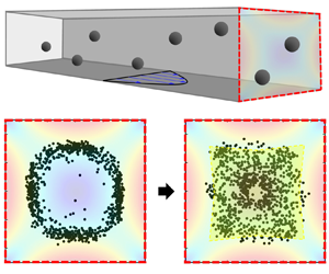
Figure 5. (a) The distribution of particles (number of particles = 1000) projected onto the y–z plane (channel cross-section) in Newtonian and Boger (500 p.p.m. PEO solution) fluids. These particle distributions were obtained at a downstream location of 4.8 cm from the channel inlet at a Reynolds number of approximately 11. The particles exhibit lateral migration and segregation in the Newtonian fluid owing to the Segré–Silberberg effect, which is significantly suppressed in the Boger fluid. The dotted lines denote the outermost boundaries where the particles cannot be present due to their finite size. (b) Assessment of spatial uniformity of particle distribution using the GSE metric. The GSE is calculated as follows:  $\textrm{GSE} ={-} (\sum\nolimits_{i = 1}^{{N_b}} {{p_i}\,\textrm{ln}\,{p_i}} )/\textrm{ln}\,{N_b}$, where
  ${N_b}$ represents the number of evenly divided bins, and
  ${p_i}$ denotes the proportion of particles in the ith bin to the total number of particles (Camesasca et al. Reference Camesasca, Kaufman and Manas-Zloczower2006). The GSE value ranges from 0 (indicating that all particles are focused in a single bin) to 1 (indicating perfect uniformity), demonstrating enhanced uniformity with increasing polymer concentration as long as the fluids are in a dilute regime (
 $c < {c^\ast }$ (858 p.p.m.)).

Figure 6. Particle distribution in 1000 p.p.m. PEO solution. The dotted lines denote the outer boundaries where the particles cannot be present due to their finite size. This result was obtained from 1000 particles at flow condition (Re = 10.4 and Wi = 287).
Previous studies have observed that the equilibrium particle positions in the elasticity-dominant flow were altered when the inertial force becomes relevant in the viscoelastic polymer solution (Yang et al. Reference Yang, Kim, Lee, Lee and Kim2011); however, whether the coexistence of inertia and elasticity leads to a uniform spatial distribution of particles has not been tested due to the limitation of visualization technique for particle location. The current experimental results observed with the dual-view system clearly demonstrate that the complex interplay between the inertial and elastic forces suppresses the Segré–Silberberg effect under inertial flow conditions.
5.2. Lateral particle migration and focusing in a cylindrical tube
Figure 7(a) shows that in the circular tube, the particles flowing in the Newtonian fluid are pinched at the location of the Segré–Silberberg annulus (Segre & Silberberg Reference Segre and Silberberg1961) with ≈ 0.55R at Re = 15. In contrast, the addition of 500 p.p.m. of PEO to the Newtonian medium results in a significantly different particle distribution compared with that in a Newtonian fluid. While the GSE analysis indicated that no discernible trend towards a more uniform cross-sectional particle distribution was observed with the addition of the polymer, the wider radial distribution of the particles in the polymer solution was evident around the equilibrium particle position (see figure 7a,b).

Figure 7. (a) Change in the particle distribution with increasing flow rate in a viscoelastic fluid (500 p.p.m. PEO solution in an aqueous solution of 22 wt% glycerine) compared with that in a Newtonian fluid (aqueous solution of 22 wt% glycerine). The flow conditions (Re and Wi numbers) significantly affected the equilibrium particle positions in the viscoelastic fluid. (b) Variation in the probability density functions with increasing flow rate as a function of the radial distance from the centre in a viscoelastic fluid and the comparison with that in a Newtonian fluid at Re = 15. (c) The diagram presenting the coefficient of two forces inducing lateral particle migration. Blue and red lines denote the inertial (fI) and elastic (fE) force coefficients in the cylindrical tube, respectively. These coefficients change as Re and Wi increase (i.e. flow rate increases).
At a low flow rate (Re = 0.54, Wi = 7.8), the particles were focused along the channel centreline in the PEO solution (figure 7a i), as previously observed in the elasticity-dominant flow condition (D'Avino et al. Reference D'Avino, Romeo, Villone, Greco, Netti and Maffettone2012). At higher flow rates, a particle-depletion region is present around the channel centre, as shown in figure 7(a,b). This phenomenon indicates that the inertial shear-gradient force overwhelms the elastic force near the channel centre as the flow rate increases. As shown in figure 7(c), the shear-gradient force drives particles from the low to high shear rate regions, namely, from the channel centre towards the wall, whereas both the elastic and inertial wall lift forces push the particles away from the wall (Ho & Leal Reference Ho and Leal1974, Reference Ho and Leal1976). The radial position of the particles is predicted to be determined by the competition of these forces, but there is still much that is not understood. In the cylindrical tube, almost all the particles (>98%) in the viscoelastic fluid are observed to exist within the range of  $r/\; R < \; 0.4$, even as the flow rate increases to Re ≈ O(101). The particle distribution in the viscoelastic fluid shows an intriguing pattern, wherein the probability distribution of particles is broader (manifested by an increase in the full-width at half-maximum (FWHM)) around the highest particle probability position (figure 7b). The probability density function (
 ${P_i}$) in the ith bin is defined as
  ${P_i} = {\hat{P}_i}/\sum\nolimits_{i = 1}^N {{{\hat{P}}_i}} $, where
  ${\hat{P}_i} = (1/{\rm \pi} (r_i^2 - r_{i - 1}^2))(\sum\nolimits_{r = {r_{i - 1}}}^{r = {r_i}} {{N_p}(r)} /\sum\nolimits_{r = 0}^{r = R} {{N_p}(r)} )$, wherein N and
  ${N_p}(r)$ represent the number of bins in the radial direction and the number of particles at r, respectively (Seo et al. Reference Seo, Byeon, Huh and Lee2014b). The outermost position where particles exist is located in the interior of the Segré–Silberberg annulus owing to the overwhelming elastic force over the inertial shear-gradient force. The broadening of particle distribution can be interpreted as a consequence of the equilibrium between shear-gradient and elastic forces: in the case of Re = 15, the relatively broad particle distribution over the wide range (
 $0.05 < r/R < 0.5$) was observed (figure 7a,b). To elucidate the underlying physics behind these experimental observations, lateral particle migration due to inertial forces is predicted by direct numerical simulation, and elasticity-driven migration is predicted by the semiempirical model (see §§ 3 and 4).
The inertial force ( ${F_I}$) exerted on a sphere can be denoted with the relationship of
  ${F_I} = {f_I}(Re,\hat{r})\rho {a^4}{(\langle u\rangle /R)^2}$ (Matas et al. Reference Matas, Morris and Guazzelli2009), and for the Newtonian fluid case, the direct numerical solution of the inertial lift coefficient,
  ${f_I}(Re,\hat{r})$, under the current experimental conditions is presented in figure 8(a) (refer to § 3 for the numerical methods). The elastic (
 ${F_E}$) forces being exerted on a spherical particle in a Boger fluid with constant shear viscosity are predicted as (4.3) using the FENE-MCR constitutive equation (Coates et al. Reference Coates, Armstrong and Brown1992) and a semiempirical scaling argument of the elastic force,
  ${F_E}\; \sim \; {a^3}\boldsymbol{\nabla }{N_1}$ (Tehrani Reference Tehrani1996; Leshansky et al. Reference Leshansky, Bransky, Korin and Dinnar2007), in a circular tube. The FENE-MCR model was adopted to consider the shear-thinning characteristics of the
  ${\varPsi _1}$. Figure 8(b) depicts the elastic force coefficients at various Wi conditions. It can be predicted that the equilibrium particle positions in the elastoinertial flow condition are determined by the sum of
  ${F_I} + {F_E}$, which yields the following relationship:
 \begin{align}
{F_I} + {F_E} & = {f_I}\rho {a^4}{\left( {\dfrac{{\langle
u\rangle }}{R}} \right)^2} - {f_E}\mu (1 - \beta )\lambda
\dfrac{{{a^3}}}{R}{\left( {\dfrac{{\langle u\rangle }}{R}}
\right)^2}\nonumber\\ & = {a^3}{\left( {\dfrac{{\langle u\rangle
}}{R}} \right)^2}\left( {{f_I}\rho a - \dfrac{{{f_E}\mu (1
- \beta )\lambda }}{R}} \right).
\end{align}
\begin{align}
{F_I} + {F_E} & = {f_I}\rho {a^4}{\left( {\dfrac{{\langle
u\rangle }}{R}} \right)^2} - {f_E}\mu (1 - \beta )\lambda
\dfrac{{{a^3}}}{R}{\left( {\dfrac{{\langle u\rangle }}{R}}
\right)^2}\nonumber\\ & = {a^3}{\left( {\dfrac{{\langle u\rangle
}}{R}} \right)^2}\left( {{f_I}\rho a - \dfrac{{{f_E}\mu (1
- \beta )\lambda }}{R}} \right).
\end{align}
Consistent with the previous theoretical approach (Matas et al. Reference Matas, Morris and Guazzelli2009), the magnitude of the inertial lift coefficient is predicted to decrease with increasing Re (figure 8a). Since the computation of  ${f_E}(Wi,{L^2},\hat{r})$ by direct numerical methods is still challenging for large Wi due to the high Weissenberg number problem in computational rheology (Keunings Reference Keunings1986), we predicted
  ${f_E}(Wi,{L^2},\hat{r})$ semiempirically (Tehrani Reference Tehrani1996). When the polymer solution is modelled with an Oldroyd-B model (
 $\,{f_E}(Wi,{L^2},\hat{r}) = {C_E}\hat{r}$ as
  ${L^2} \to \infty $), the net force is always negative in sign, and its magnitude increases in proportion to the Re number (black plots in figure 9). Therefore, the particle stream, that was once focused along the centreline owing to the dominance of the elastic force over the inertial force at low Re (Re = 0.54; Wi = 7.8), is expected to remain unaffected even with increasing flow rate (Re
  $\uparrow $ and Wi
  $\uparrow $). This can be deduced from the following argument: for the Oldroyd-B model, the magnitude of
  ${f_I}(Re,\hat{r})$ decreases with increasing flow rate (Matas et al. Reference Matas, Morris and Guazzelli2009), while the other terms remain fixed at the same radial location in (5.1). In this case, the equilibrium particle position that forms at the centre is not expected to change even as the flow rate increases. The elastic force becomes more dominant over the inertial force near the channel centre with increasing flow rate in the case of the Oldroyd-B model, which is in contrast to the significant change in lateral particle distribution found experimentally in this study. Given the finite extensibility of the polymer (
 ${L^2}$), it can be observed in figure 8(b) that as Wi increases,
  ${f_E}(Wi,{L^2},\hat{r})$ deviates significantly from the linear relationship with a decreasing slope as it approaches the wall from the channel centre. The nonlinearity in the FENE-MCR model predicts that the net force distribution in the r direction becomes flat and is markedly different from the Oldroy-B model case, as shown in figure 9. Note that when
  ${L^2} = 6942$ (estimated from the maximum and minimum length scales of the 2M PEO conformation), the net force is still negative in all r locations: the net force acts only towards the centre (red plots in figure 9) under all flow conditions, therefore, which cannot account for the current experimental results. Therefore, we also considered the
  ${L^2} = 10$ case much smaller than
  ${L^2} = 6942$, since it was previously shown that the values much smaller than
  ${L^2}$, obtained from the relative ratio of the polymer contour length to radius of gyration, were demanded to match the numerical simulation with the experimental data. When
  ${L^2} = 10$, it was observed that a region, where the net force is positive, appears near the centre as Re increases (blue plots in figure 9). Although the region
  $r/R < 0.1$ still shows that the net force is negative even at Re = 15, considering the finiteness of the PS bead size (
 $a/R = 0.12$), it becomes evident that the net force exerted on the particle near the channel centre is directed towards the channel wall. Consequently, the particle-depletion region is predicted to be formed at the channel centre as experimentally observed (figure 7a,b). However, it is evident that not all experimental results can be explained simply by adjusting
  ${L^2}$ in the FENE-MCR model. To obtain results that are more consistent with experimental results, it may be necessary to introduce a multimode model that can more accurately describe the shear rate dependence of the first normal stress difference (McKinley et al. Reference McKinley, Armstrong and Brown1993). Nevertheless, when the viscoelastic flow is modelled with the FENE-MCR model, it was found that the net zero location of the inertial and elastic forces can be formed inside the Segré–Silberberg annulus, which supports the current experimental findings (cf. Re = 10 case for
  ${L^2} = 10$ in figure 9). Furthermore, it is notable that for
  $L^2 = 10$ in the FENE-MCR model, a region is observed where the sum of the inertial and elastic forces is nearly zero at Re = 5. This phenomenon corresponds to the broad particle distribution observed in the experimental results (figure 7a,b). This spatially broad distribution region is confined within the Segré–Silberberg annulus by the sum of the elastic and inertial wall lift forces acting from the wall to the channel centre (refer to figure 7c). In short, our findings indicate that the nonlinear distributions of the elastic force, which is predicted from the FENE-MCR model (as shown in figure 8b; (4.3) and (4.4)), are the possible origin for the particle-depletion region and broad particle distribution observed in the Boger fluid in the cylindrical tube.

Figure 8. The plots of inertial (fI) and elastic (fE) force coefficient in the Oldroyd-B and FENE-MCR models as a function of normalized radial location ( $\hat{r} = \; r/R$) at different flow conditions. (a) Inertial force coefficient (fI) obtained with direct numerical simulation (see § 3) with regression (solid lines). (b) Elastic force coefficients (
 $\,{f_E}$) predicted with Oldroyd-B model and FENE-MCR model with different finite extensibility of polymer chain (
 ${L^2}$). When
  ${L^2}$ approaches infinity, the FENE-MCR model is reduced to the Oldroyd-B model (black-dash line) showing a linear relationship between
  ${f_E}$ and
  $\hat{r}$ irrespective of Wi number. The solid lines correspond to
  ${f_E}$ predicted with FENE-MCR model when
  ${L^2} = 6942$ (
 ${C_E} = 8.66$).

Figure 9. The net force distributions across the radial direction, obtained with the application of (5.1), are illustrated in (a). Panel (b) corresponds to a zoom-in view of the data presented in (a) (designated with a double-headed red arrow). The blue, red and black symbol data correspond to  ${L^2} = 10$, 6942 and
  $\infty $ cases in the FENE-MCR model, respectively, where the
  ${L^2} = \infty $ case is equivalent to the Oldroyd-B model.
5.3. Mechanism for the suppression of the Segré–Silberberg effect in a square channel
In the cylindrical tube, we observed the formation of a force-balanced zone through the compensation of shear-gradient and elastic forces. However, the homogenization of the spatial particle distribution, which was observed in a square channel (figure 5), does not occur in the case of the circular channel. Therefore, we expect that the non-axisymmetric flow kinematics inherent to the square channel significantly influence the spatial particle distribution. To elucidate the origin of the homogenization of particle distribution induced by the addition of polymers, we investigated the particle distribution within the square channel with increasing the flow rate (figure 10a). At a low flow rate (Q = 0.04 ml h−1), the particles moving along the channel centreline and its four corners transit into the focusing along the centreline as the flow increases to Q = 0.2 ml h−1, commonly referred to as elastoinertial particle focusing (refer to figure 10b), which is consistent with those in a previous observation (Yang et al. Reference Yang, Kim, Lee, Lee and Kim2011).

Figure 10. (a) Probability distribution in the cross-section of a square channel in a viscoelastic fluid (500 p.p.m. 2M PEO solution in an aqueous solution of 22 wt% glycerine) obtained with the dual-view imaging system (the probability distribution at a flow rate of 6 ml h−1; the same data as in figure 5(a) is used here for comparison). (b) Schematic to elucidate the mechanism for the suppression of the Segré–Silberberg effect, combined with strain rate distribution (unit s−1) in the square channel. (i) Equilibrium particle positions by the elastic dominant and (ii) elastoinertial particle migration mechanisms have previously been reported in a square channel (Yang et al. Reference Yang, Kim, Lee, Lee and Kim2011), which are consistent with the particle distributions observed at flow rates of 0.04 and 0.2 ml h−1 in this study, respectively. The regions with lower shear rate exist along the diagonal directions in the square channel, in contrast to those in a circular tube. (iii) Both orthogonal and diagonal shear rate gradients occur owing to these regions, resulting in particle accumulation along the channel diagonal directions owing to the combined effects of elastic and shear-gradient inertial forces. (iv) Furthermore, if the flow rate is increased beyond 4 ml h−1, the two forces cancel each other out, leading to a spatially uniform distribution of particles observed in (a).
Unlike in the case of a circular conduit, a significant distinction arises in the square channel owing to its non-axisymmetric nature, leading to the existence of regions with lower shear rates in the diagonal direction (shear rate distribution background in figure 10b) (Yang et al. Reference Yang, Kim, Lee, Lee and Kim2011). Similar to the observations in the circular conduit, with the further increase in the flow rate, the shear-gradient force surpasses the elastic force near the centre region. This causes particles at the channel centre to move outward from the channel centre. Meanwhile, as shown in figure 10(b), the presence of low shear rate regions in the diagonal direction accounts for the elastic forces pushing particles towards these regions ( ${F_E}\sim {a^3}\boldsymbol{\nabla }{N_1}(\dot{\gamma })$) (Yang et al. Reference Yang, Lee, Ahn, Kang, Shim, Lee, Hyun and Kim2012). Therefore, as the flow rate is increased to the volumetric flow rate (Q) = 1.0–2.0 ml h−1, the particle-depletion region emerges at the channel centre, simultaneously exhibiting a characteristic region where particles are diagonally distributed owing to the elastic force. When the flow rate is further increased to Q = 4.0–6.0 ml h−1, the particles that were originally diagonally located are dispersed in the normal directions of diagonal lines owing to the balance between the shear-gradient and the elastic forces. This force equilibrium creates a spatial force-balanced zone, explaining the spatially uniform particle distribution that is observed in this study. This tendency for the particles to disperse in the diagonal region with increasing Re and Wi numbers was identical in all the Boger fluids below c = 500 p.p.m. (El = 14.4); however, the exact shapes of the distribution were different with varying concentrations of the polymer additive (figure 11). Meanwhile, at the higher polymer concentration (c = 1000 p.p.m.), as the elasticity is more relevant than the inertial shear-gradient force (El = 27.6), particles are still present at the channel centre and their spreading out in the directions perpendicular to the diagonals was slightly reduced (figure 6). A supplementary experiment was conducted with a 500 p.p.m. solution to ascertain whether the current channel length is adequate for achieving a steady-state particle distribution. This was accomplished by comparing the distributions of particles at the locations of 4 and 4.8 cm downstream from the channel inlet. The distributions exhibited no significant difference, as shown in supplementary figure S4. This finding validates the use of 4.8 cm downstream from the inlet for observing the steady-state particle distribution. Additionally, we found no secondary flow effect in the Boger fluid from the fluorescent mixing test as shown in supplementary figure S5, indicating that only inertial and elastic forces contribute to the lateral particle migration.

Figure 11. Particle distributions in Newtonian and Boger fluids (100, 250 and 500 p.p.m. PEO solutions) according to Reynolds (Re) and Weissenberg (Wi) numbers. All the figures show the distributions of at least 200 particles (the particle distributions in row (c) and column (iv) (500 p.p.m. PEO solution) were obtained from 1000 particles; the data presented in the main text are shown here for comparison).
These results show that the inhomogeneity of the spatial distribution of particles caused by inertial forces can be suppressed by the non-axisymmetric inertial force and elastic effect induced by polymer additive with its optimal concentration without any other significant effects. This study provides clear evidence that, in addition to the ability to control the number of equilibrium particle positions through the manipulation of elasticity and inertia in polymer solutions – a phenomenon that has been explored in the existing literature (Yang et al. Reference Yang, Kim, Lee, Lee and Kim2011) – it is also possible to achieve particle homogenization by leveraging the inertial and elastic forces acting in opposite directions. It can also be deduced from existing numerical analyses (Li, McKinley & Ardekani Reference Li, McKinley and Ardekani2015) that the inertia and elastic forces can be net zero. In the previous study (Yang et al. Reference Yang, Kim, Lee, Lee and Kim2011), it has been observed that at specific flow rates, particles are focused along the centre line of the channel. However, at higher flow rates, the particle focusing was observed to diminish. However, as the particle distribution was only observed in two dimensions, it was not possible to conclude whether the particle distribution became uniform in the channel cross-section or whether the line equilibrium positions across the channel width direction were formed. By utilizing the dual-view microscope system developed in this study, it was confirmed that the particle distribution is homogenized by the balance of elasticity and inertia forces in a rectangular channel, in contrast to a round channel.
6. Conclusion
This study investigated the lateral particle distribution in the pressure-driven flows of viscoelastic polymer solutions using a dual-view imaging system to determine the particle locations in the channel cross-section. In pressure-driven flow, inertia and elasticity are known, respectively, to move particles in the lateral direction across the main-stream flow, thereby spatially redistributing the particles to specific locations. However, through this study, we demonstrated that the Segré–Silberberg effect, which inevitably occurs under inertial flow conditions, can be suppressed in a square channel owing to the offset between inertial and elastic forces. In order to gain insight into the variation of inertial and elastic forces with flow rate, the experimental findings in a circular channel were analysed using direct numerical simulation of inertial force and semiempirical modelling for the elastic force. The experimental results obtained in the circular channel indicate that as the flow rate is increased, the particles tend to disperse from the centre after being focused along the channel centreline at low flow rates. The comparison between experimental and modelling results revealed that the nonlinearity of the elastic force due to the finite extensibility of polymers plays a pivotal role in the offset of the inertial and elastic forces. On the other hand, the non-axisymmetric shear rate distribution induces a multitude of directional offsets of the inertial and elastic forces in a square channel, resulting in a more uniform particle distribution than that observed in a circular channel. It is expected that the design of channel cross-section geometry for more uniform particle distribution can be achieved using the direct numerical simulations such as finite element analysis (Villone et al. Reference Villone, D'Avino, Hulsen, Greco and Maffettone2013). However, to conduct numerical simulations at Wi ≈ O(102) encountered in this study, the so-called high Weissenberg number problem (Keunings Reference Keunings1986) must be addressed as a prerequisite, although it has been partially resolved with modern numerical techniques, such as log-conformation formulation (Fattal & Kupferman Reference Fattal and Kupferman2005). Finally, the addition of a polymer apparently has a similar effect on the lateral motion of particles, as if reducing the Re value. This analogy can be drawn to the well-known phenomenon of turbulent drag reduction in fluid dynamics, achieved by suppressing the turbulent characteristics through polymer addition.
Supplementary material
Supplementary material is available at https://doi.org/10.1017/jfm.2024.1234.
Acknowledgements
The authors are grateful to Professor P.S. Doyle at MIT for his suggestion to quantify the spatial uniformity of particles.
Funding
This study was supported by the National Research Foundation of Korea (NRF) grants funded by the Korean government (RS-2023-00241646 and NRF-2018R1A5A1024127).
Declaration of interests
A Korean patent application (10-2022-0031304) has been filed for the dual-view imaging system.
Author contributions
J.M.K. and D.J. conceived the project. J.M.K., D.J. and J.I.P. designed the experiments. D.J. conducted the microfluidic experiments. All authors contributed to the analysis of the experimental data. J.M.K., D.J., Y.K. and J.B.Y. contributed to the development of the quantification method for the uniformity of spatial particle distribution. D.J., J.I.P. and J.M.K. contributed to the measurement and interpretation of the rheological data. H.M.L., D.J., J.I.P. and J.M.K. contributed to the numerical and modelling works. All authors wrote the manuscript and commented on it. J.M.K. supervised the project.
Data availability
The data that support the findings of this study are available from the corresponding author upon reasonable request.


