


1. Introduction
1.1. Broader context
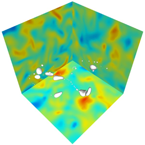
Chemical, aerosol and gas exchanges through liquid–gas interfaces appear in numerous industrial and environmental situations. In many cases, the interface deforms and breaks violently under the action of turbulent flows forming drops and bubbles (Eggers & Villermaux Reference Eggers and Villermaux2008; Balachandar & Eaton Reference Balachandar and Eaton2010). The newly formed satellite interfaces increase drastically the exchange surface, enhancing the transfer between the two phases. Practical examples include oil spill mitigations (Gopalan & Katz Reference Gopalan and Katz2010; Afshar-Mohajer et al. Reference Afshar-Mohajer, Li, Rule, Katz and Koehler2018), oil and gas transportation from remote wells (Galinat et al. Reference Galinat, Masbernat, Guiraud, Dalmazzone and Noı2005; Ayati et al. Reference Ayati, Farias, Azevedo and de Paula2017), air entrained by bow waves in naval applications (Baba Reference Baba1969; Shakeri, Tavakolinejad & Duncan Reference Shakeri, Tavakolinejad and Duncan2009), together with ocean–atmosphere interactions with breaking waves inducing bubble-mediated gas exchange (Deane & Stokes Reference Deane and Stokes2002; Deike, Lenain & Melville Reference Deike, Lenain and Melville2017; Deike & Melville Reference Deike and Melville2018) and ejecting sea spray aerosols (Veron Reference Veron2015).
The description of bubbles generated by breaking waves is of first interest in the understanding of the interactions between atmosphere and oceans (Wallace & Wirick Reference Wallace and Wirick1992; Melville Reference Melville1996). Bubbles have a dramatic effect on gas transfer, accounting for 30 % to 40 % of the total CO2 gas transfer between the ocean and the atmosphere (Keeling Reference Keeling1993; Deike & Melville Reference Deike and Melville2018; Reichl & Deike Reference Reichl and Deike2020) and acting as the main pathways for low solubility gases (Liang et al. Reference Liang, McWilliams, Sullivan and Baschek2011). The smallest bubbles tend to dissolve in the water whereas larger ones rise to the surface and collapse. The bursting of bubbles at the surface produces sea spray aerosol, that can be transported in the atmosphere and evaporate, playing a role in the thermodynamics of the atmosphere (Veron Reference Veron2015). As a consequence, improving the accuracy of Earth system models requires an improved description of turbulent air–water flows.
The break-up of bubbles can be controlled by interfacial instabilities or triggered by turbulent fluctuations at the particle scale, with fragmentation in turbulence being a major research challenge in multi-phase flows (Elghobashi Reference Elghobashi2019; Villermaux Reference Villermaux2020). Earlier studies have concentrated on identifying the stable bubble length scale, from a balance between turbulent pressure fluctuations and interfacial forces (Kolmogorov Reference Kolmogorov1949; Hinze Reference Hinze1955; Risso & Fabre Reference Risso and Fabre1998; Martinez-Bazan, Montanes & Lasheras Reference Martinez-Bazan, Montanes and Lasheras1999a,Reference Martinez-Bazan, Montanes and Lasherasb). The turbulent kinetic energy at the particle scale, assuming it is within the inertial range, only depends on the turbulent dissipation rate (Kolmogorov Reference Kolmogorov1941), and the comparison between the turbulence and surface tension forces at the bubble scale defines the Weber number. Below a critical Weber number,  $We_c$, surface tension forces will prevent bubble break-up while at larger Weber number, bubble break-up can occur (Kolmogorov Reference Kolmogorov1949; Hinze Reference Hinze1955; Risso & Fabre Reference Risso and Fabre1998; Martinez-Bazan et al. Reference Martinez-Bazan, Montanes and Lasheras1999a,Reference Martinez-Bazan, Montanes and Lasherasb). The Weber number can also be interpreted in terms of the ratio between the capillary and inertial time scales. The critical Weber number defines the Hinze size,
  $d_h$,
  $We_c\equiv We(d_h)$ which can also be derived by dimensional analysis, balancing the turbulence and surface tension forces (Kolmogorov Reference Kolmogorov1949; Hinze Reference Hinze1955). Experimental studies of bubble dynamics in turbulence have measured the critical Weber number and found values of order unity. Two mechanisms driving the deformation and break-up have been discussed (Martinez-Bazan et al. Reference Martinez-Bazan, Montanes and Lasheras1999a; Andersson & Andersson Reference Andersson and Andersson2006; Ravelet, Colin & Risso Reference Ravelet, Colin and Risso2011; Vejražka, Zedníková & Stanovskỳ Reference Vejražka, Zedníková and Stanovskỳ2018), namely either direct strong action of an eddy at the scale of the bubble leading to large deformation and break-up, or a resonance mechanism between deformation caused by weaker eddies and oscillation of the bubble (Risso & Fabre Reference Risso and Fabre1998). Experimental studies have identified an oscillatory response of bubbles in turbulence associated with the second eigenmode in the spherical harmonic decomposition (Risso & Fabre Reference Risso and Fabre1998; Ravelet et al. Reference Ravelet, Colin and Risso2011; Perrard et al. Reference Perrard, Rivière, Mostert and Deike2021). This leads to a modification of the Kolmogorov–Hinze theory (Hinze Reference Hinze1955), i.e. a critical Weber number is identified and the break-up time is related to the turbulent time, or eddy turnover time, at the size of the parent bubble, and decreases with increasing Weber number, with possible finite-Reynolds-number corrections (Martinez-Bazan et al. Reference Martinez-Bazan, Montanes and Lasheras1999a,Reference Martinez-Bazan, Montanes and Lasherasb; Revuelta, Rodríguez-Rodríguez & Martínez-Bazán Reference Revuelta, Rodríguez-Rodríguez and Martínez-Bazán2006; Martinez-Bazan et al. Reference Martinez-Bazan, Rodriguez-Rodriguez, Deane, Montañes and Lasheras2010).
The break-up of bubbles close to the critical conditions, i.e. close to the critical Weber number, has received considerable attention. The observed critical Weber number varies by almost an order of magnitude (Risso & Fabre Reference Risso and Fabre1998; Martinez-Bazan et al. Reference Martinez-Bazan, Montanes and Lasheras1999a; Risso Reference Risso2000; Andersson & Andersson Reference Andersson and Andersson2006; Galinat et al. Reference Galinat, Risso, Masbernat and Guiraud2007; Liao & Lucas Reference Liao and Lucas2009; Ravelet et al. Reference Ravelet, Colin and Risso2011; Vejražka et al. Reference Vejražka, Zedníková and Stanovskỳ2018), which could be attributed to the large differences in experimental conditions (e.g. turbulence created by falling jets, at the core of a turbulent jet, under breaking waves), together with variability in estimating the turbulent dissipation rate (single point measurements, spatial average over potentially non-homogenous regions, local anisotropy in the flow), while the level of homogeneity and isotropy of the turbulent flow can also vary by large degrees. This complicates direct comparison and makes extrapolation to inhomogeneous turbulence encountered in nature almost impossible. Mostly binary break-up models have been considered in population balance approaches (Martinez-Bazan et al. Reference Martinez-Bazan, Rodriguez-Rodriguez, Deane, Montañes and Lasheras2010; Qi, Masuk & Ni Reference Qi, Masuk and Ni2020). The break-up of bubbles far from the critical size exhibits very different behaviour, with the formation of multiple satellite bubbles below the critical Hinze scale, and remains poorly characterized.
Separately, the size distribution of bubbles under a breaking wave has been studied experimentally (Loewen & Melville Reference Loewen and Melville1994; Deane & Stokes Reference Deane and Stokes2002; Rojas & Loewen Reference Rojas and Loewen2007; Blenkinsopp & Chaplin Reference Blenkinsopp and Chaplin2010) and more recently numerically (Deike, Melville & Popinet Reference Deike, Melville and Popinet2016). Experimental and numerical results exhibit a power law scaling for the bubble size distribution above the Hinze scale,  $d>d_h$, following
  $N(d)\propto d^{-10/3}$, which can be rationalized by a turbulent cascade model developed by Garrett, Li & Farmer (Reference Garrett, Li and Farmer2000). This model is based on the idea of bubble fragmentation cascade by turbulence, with a break-up time given by the eddy turnover time at the size of the parent bubble and local production sizes. However, for bubbles below the critical Hinze scale,
  $d<d_h$, the statistics remain poorly characterized, with experimental data exhibiting large variations (see figure 1 of Deike et al. (Reference Deike, Melville and Popinet2016) showing variations in bubble size distributions from experimental results by Loewen & Melville (Reference Loewen and Melville1994), Deane & Stokes (Reference Deane and Stokes2002), Rojas & Loewen (Reference Rojas and Loewen2007) and Blenkinsopp & Chaplin (Reference Blenkinsopp and Chaplin2010)) and the formation mechanisms still to be determined. Such sub-Hinze scale bubbles correspond to scales from the micron to the millimetre scale, which contribute the most to gas exchange (Deike & Melville Reference Deike and Melville2018), especially for low solubility gases (Keeling Reference Keeling1993), and aerosol generation through bubble bursting (Veron Reference Veron2015).
Direct modelling of bubble deformation and break-up in a turbulent flow is a challenging task, and an extensive review on the various numerical approaches for droplet and bubble of various sizes in turbulence has recently been presented by Elghobashi (Reference Elghobashi2019). Numerical methods to study the deformation of bubbles or droplets larger than the Kolmogorov length scale in a turbulent flow are especially challenging as they need to resolve the shape and motion of the interfaces between the two phases. Three families of methods have been employed (Elghobashi Reference Elghobashi2019). (I) Front-tracking methods, where the interface is marked by points that are advected by the flow, as in the front-tracking method of Unverdi & Tryggvason (Reference Unverdi and Tryggvason1992) and Tryggvason et al. (Reference Tryggvason, Bunner, Esmaeeli, Juric, Al-Rawahi, Tauber, Han, Nas and Jan2001) which have been used to study the deformation of large bubbles in turbulence (Lu & Tryggvason Reference Lu and Tryggvason2008, Reference Lu and Tryggvason2013). (II) Immersed boundary methods were recently used by Spandan, Verzicco & Lohse (Reference Spandan, Verzicco and Lohse2018) to perform a direct numerical simulation (DNS) study on the effects of dispersed deformable bubbles larger than the Kolmogorov scale on drag reduction in a turbulent Taylor–Couette flow. (III) Tracking scalar function methods, which come with different interface reconstruction methods, (i) the volume of fluid method where the relevant function is the volume fraction of the local phase on either side of the interface (Scardovelli & Zaleski Reference Scardovelli and Zaleski1999), (ii) the level-set method, where the function is the signed distance function representing the distance from the interface (e.g. Desjardins, Moureau & Pitsch Reference Desjardins, Moureau and Pitsch2008), (iii) the lattice Boltzmann method, which uses a probability density function of finding a fluid particle of fluid phase within the discretized lattice (Shan & Chen Reference Shan and Chen1993; Chen & Doolen Reference Chen and Doolen1998) and (iv) the phase field method, where the function is the scalar phase field, which represents one of the physical properties (e.g. molar concentration) of a binary fluid mixture. The function is mostly uniform in the bulk phases and varies smoothly over a diffuse interfacial layer of finite thickness, with its transport governed by the Cahn–Hilliard equation (Cahn & Hilliard Reference Cahn and Hilliard1959).
The break-up of an interface in turbulence has been achieved using scalar functions methods. Simulations of single-bubble deformation and break-up in isotropic turbulence using the lattice Boltzmann method were performed by Qian et al. (Reference Qian, McLaughlin, Sankaranarayanan, Sundaresan and Kontomaris2006). The results were compared to Risso & Fabre (Reference Risso and Fabre1998) in terms of deformation and confirmed the identification of a critical Weber number. More recently, Mukherjee et al. (Reference Mukherjee, Safdari, Shardt, Kenjereš and Van den Akker2019) used the lattice Boltzmann method to study droplet–turbulence interactions and quasi-equilibrium dynamics in turbulent emulsions. Rising deformable bubbles in turbulence have been studied by Loisy & Naso (Reference Loisy and Naso2017) with a modified level-set method. Soligo, Roccon & Soldati (Reference Soligo, Roccon and Soldati2019) used the phase field approach to study the breakage, coalescence and size distribution of surfactant-laden droplets in a turbulent flow. These recent studies observed a droplet size distribution following a  $d^{-10/3}$ scaling for particles larger than the critical Hinze scale. Such distributions had previously been reported to describe the bubble size distribution under a breaking waves, both experimentally (Deane & Stokes Reference Deane and Stokes2002) and through DNS using the volume of fluid (VOF) approach (Deike et al. Reference Deike, Melville and Popinet2016; Wang, Yang & Stern Reference Wang, Yang and Stern2016). It has also been successfully used to study complex two-phase turbulence flow under breaking waves (Deike et al. Reference Deike, Melville and Popinet2016; Wang et al. Reference Wang, Yang and Stern2016; Chan et al. Reference Chan, Johnson, Moin and Urzay2021), and allows us to reach high density and viscosity ratios. Additionally, the VOF algorithm has also been used to study a large number of droplets being deformed and interacting with the turbulent flow (Dodd & Ferrante Reference Dodd and Ferrante2016).
Here, we investigate the break-up of bubbles in a homogeneous and isotropic turbulent flow by direct numerical simulations of the two-phase, three-dimensional, incompressible Navier–Stokes equations with surface tension, and a geometric VOF method to reconstruct the interface, making use of the recent progresses in numerical methods implemented in the Basilisk package (van Hooft et al. Reference van Hooft, Popinet, van Heerwaarden, van der Linden, de Roode and van de Wiel2018; Popinet Reference Popinet2018). We use a spatial adaptive octree grid to investigate bubble break-up resolving for a wide range of scales, as recently demonstrated for two-phase turbulent flow in the case of breaking waves (Deike et al. Reference Deike, Melville and Popinet2016; Mostert & Deike Reference Mostert and Deike2020). This work focuses on bubble break-up and explores the formation of sub-Hinze scale bubbles while a companion paper describes the deformation dynamics prior to breaking (Perrard et al. Reference Perrard, Rivière, Mostert and Deike2021).
1.2. Setting the scene
We consider a bubble of diameter  $d_0$, density
  $\rho _a$ and viscosity
  $\mu _a$ in a turbulent liquid of density
  $\rho _w$ and viscosity
  $\mu _w$, and
  $\gamma$ is the surface tension coefficient between air and water. We work with the air–water density ratio
  $\rho _w/\rho _a=850$ and a high viscosity ratio of
  $\mu _w/\mu _a=25$.
The break-up dynamics of a bubble in a turbulent flow depends primarily on the ability of the surrounding fluid to deform the bubble against surface tension forces. This defines the Weber number, comparing inertial forces generated by the turbulent carrier flow and the capillary cohesive forces. Considering the velocity fluctuation at the bubble diameter scale  $d_0$, formalized by the longitudinal velocity increment
  $\delta u(d_0) = u_L(r,t) - u_L(r+d_0,t)$, the turbulent Weber number is defined as
  $We = \rho _w \langle \delta u(d_0)^2 \rangle d_0/\gamma$ (Hinze Reference Hinze1955; Risso & Fabre Reference Risso and Fabre1998) with
  $\rho _w$ the density of water,
  $\gamma$ the air–water surface tension and
  $\langle \rangle$ the average over the flow configurations. In a homogeneous and isotropic turbulent flow, the velocity fluctuations at the bubble scale
  $\delta u(d_0)^2$ can be related to the mean dissipation rate of energy
  $\epsilon$ using the Kolmogorov (Reference Kolmogorov1941) theory
  $\langle \delta u(d_0)^2 \rangle = C (\epsilon d_0)^{2/3}$ for
  $d_0$ in the inertial range. Experimental studies have observed
  $C \in [2,2.2]$ depending on Reynolds number (Pope Reference Pope2000; Cowen & Variano Reference Cowen and Variano2008). We chose
  $C=2$ for consistency with Risso & Fabre (Reference Risso and Fabre1998), and the Weber number writes,
 \begin{equation} We = \frac{2\rho_w \epsilon^{2/3}d_0^{5/3}}{\gamma}. \end{equation}
 The critical Weber number,  $We_c$ below which the bubble might deform but does not break, defines the Hinze scale
  $d_h$ (Hinze Reference Hinze1955; Risso & Fabre Reference Risso and Fabre1998), so that
  $We_c\equiv We(d_h)$, and it follows,
 \begin{equation} d_h=\left(\frac{We_c}{2}\right)^{3/5}\left(\frac{\gamma}{\rho_w}\right)^{3/5}\epsilon^{{-}2/5}. \end{equation}
 This assumes that the bubble is within the inertial range. In essence, the turbulent flow presents large fluctuations, leading to a broad range of break-up times for the same turbulent conditions, especially close to stable conditions, which make estimations of the critical Weber number challenging. The critical Hinze scale (or critical Weber number) is usually defined in a statistical sense and for a given time of observation, typically corresponding to the conditions where half of the bubbles will break while the other half will not break. This definition thus depends on an observation time constrained by experimental procedures (or numerical limitations), which is one of the reasons for the variations in the literature. The experimentally reported values of the critical Weber numbers are typically between 0.7 and 5 (Risso & Fabre Reference Risso and Fabre1998; Martinez-Bazan et al. Reference Martinez-Bazan, Montanes and Lasheras1999a; Deane & Stokes Reference Deane and Stokes2002; Andersson & Andersson Reference Andersson and Andersson2006; Liao & Lucas Reference Liao and Lucas2009; Vejražka et al. Reference Vejražka, Zedníková and Stanovskỳ2018) corresponding to variations in the pre-factor  $(We_c/2)^{3/5}$ from approximately 0.5 to 2. The wide range of critical Weber numbers observed can also be related to the variability in the experimental configurations, which introduces other flow parameters, such as large scale shear or spatial variations of the dissipative rate
  $\epsilon$. As will be discussed later in the paper, we obtain and consider a value of
  $We_c=3$ in our numerical configuration, which we will use throughout the paper, that falls into the experimentally reported values.
Building on earlier work (Hinze Reference Hinze1955; Risso & Fabre Reference Risso and Fabre1998; Martinez-Bazan et al. Reference Martinez-Bazan, Montanes and Lasheras1999a), Perrard et al. (Reference Perrard, Rivière, Mostert and Deike2021) and Ruth et al. (Reference Ruth, Mostert, Perrard and Deike2019) discuss the relevant time scale for bubble deformation and break-up. In particular, the eddy turnover time at the scale of the bubble, or turbulent time scale at the size of the bubble  $d_0$ is given by
 \begin{equation} t_c = d_0^{2/3}\epsilon^{{-}1/3}. \end{equation}
As discussed by Perrard et al. (Reference Perrard, Rivière, Mostert and Deike2021) and in agreement with experimental observation, this provides a reasonable estimate of the break-up time at high Weber number ( $We\gg We_c$) while the distribution of break-up times close to stable conditions is very broad.
The second controlling parameter is the intensity of the turbulent flow, characterized by the Reynolds number  $Re$, the ratio between inertial forces and viscous forces. The turbulent flow fluctuations are better characterized by the Taylor Reynolds number, which is based on the correlation length of velocity gradients, called the Taylor micro-scale. In homogeneous and isotropic turbulence, the Taylor micro-scale reads (Pope Reference Pope2000)
  $\lambda = \sqrt {(15 \mu _w)/(\rho _w \epsilon )} u_{rms}$, with
  $u_{rms}$ the root mean square of the velocity. The Taylor Reynolds number is defined as (Pope Reference Pope2000),
 \begin{equation} Re_{\lambda} = \frac{\rho_w u_{rms} \lambda}{\mu_w}.\end{equation}
The use of these definitions from single-phase homogeneous and isotropic turbulence is justified by the low volume fraction of air considered.
The influence of the Reynolds number on the break-up process, break-up time and child size distribution has been less studied than the effect of the Weber number, which is the main controller of the break-up processes (Hinze Reference Hinze1955; Risso & Fabre Reference Risso and Fabre1998; Martinez-Bazan et al. Reference Martinez-Bazan, Rodriguez-Rodriguez, Deane, Montañes and Lasheras2010). Note that gravity,  $g$, can affect the break-up for large rising bubbles (Magnaudet & Eames Reference Magnaudet and Eames2000; Ravelet et al. Reference Ravelet, Colin and Risso2011), and is quantified by the Bond number
  $Bo=(\rho _w g d_0^2)/\gamma$, but is not considered in the present work.
1.3. Outline of the present work: bubble break-up in turbulence
We study bubble break-up in continuously forced conditions, within a stationary homogenous and isotropic turbulent flow. The continuously forced conditions mimic the natural or experimental conditions where multiple break-up events may happen successively, leading to a final distribution of child bubbles. We investigate the role of the Weber number on the break-up dynamics and child size distribution. The Weber number is increased from a low value with deformation but no-break-up ( $We\ll We_c$), to break-up close to critical Weber number (
 $We\geq We_c$) and up to large Weber number with dramatic break-up (
 $We\gg We_c$). The principle of the simulations is the following. We insert a bubble into a turbulent flow and characterize its deformation, break-up times and child formation. We present both a dynamical discussion of the break-up processes through analysis of single simulations at high resolution and a statistical analysis of the resulting size distribution obtained from averaging an ensemble of simulations and events.
The paper is organized as follow. First, in § 2, we present the computational methods, and discuss the creation of an isotropic homogeneous turbulent flow through a precursor simulation with no bubble and finally the insertion of the bubble. We verify convergence of the turbulent flow and the bubble dynamics in decaying turbulence for an increasing maximum level of resolution. In § 3, we introduce the ensemble of continuously forced turbulence simulations done at different initial Weber numbers and interface resolutions. We present the phenomenology on increasing the Weber number, from break-up close to stable conditions, which only produces a few bubbles, to high Weber number conditions where multiple break-ups are observed, leading to the formation of a wide range of bubbles, in particular numerous sub-Hinze scale bubbles. In § 4, we discuss the statistics of child bubbles during the multiple break-ups and the final size distribution. We discuss the local and non-local production mechanisms in scale and conclude in § 5.
2. The numerical configuration: solver, creation and characterization of the turbulent flow and bubble injection
2.1. Numerical methods: the Basilisk flow solver
We perform direct numerical simulations of the three-dimensional, incompressible Navier–Stokes equations, either with a single phase (the turbulence precursor simulation) or with two phases (air bubble and turbulent water) with surface tension. We use the free software Basilisk (http://basilisk.fr/), the successor of Gerris, which is based on a spatial adaptive quad-octree grid allowing us to save computational time while resolving the different length scales of the problem (Popinet Reference Popinet2003, Reference Popinet2009). It is based on a momentum conserving scheme and a sharp VOF method to reconstruct the interfaces (Popinet Reference Popinet2018) between the high density liquid (water) and the low density gas (air). These methods have been extensively described in recent publications (Popinet Reference Popinet2015, Reference Popinet2018; Fuster & Popinet Reference Fuster and Popinet2018; van Hooft et al. Reference van Hooft, Popinet, van Heerwaarden, van der Linden, de Roode and van de Wiel2018), and their accuracy has been validated, with multiple examples and test cases available on the Basilisk website, with studies exploring complex multiphase flow, including splashing (Thoraval et al. Reference Thoraval, Takehara, Etoh, Popinet, Ray, Josserand, Zaleski and Thoroddsen2012; Marcotte et al. Reference Marcotte, Michon, Séon and Josserand2019), bubble bursting (Deike et al. Reference Deike, Ghabache, Liger-Belair, Das, Zaleski, Popinet and Seon2018; Lai, Eggers & Deike Reference Lai, Eggers and Deike2018; Berny et al. Reference Berny, Deike, Séon and Popinet2020), instability at an interface (Bagué et al. Reference Bagué, Fuster, Popinet, Scardovelli and Zaleski2010), and wave breaking (Deike, Popinet & Melville Reference Deike, Popinet and Melville2015; Deike et al. Reference Deike, Melville and Popinet2016, Reference Deike, Lenain and Melville2017; Mostert & Deike Reference Mostert and Deike2020; Mostert, Popinet & Deike Reference Mostert, Popinet and Deike2021). Note that compressible effects in the bubble dynamics are not considered here.
The multi-fluid interface is traced by a function  $\mathcal {T}(\boldsymbol {x},t)$, defined as the volume fraction of a given fluid in each cell of the computational mesh. The density and viscosity can thus be written as
  $\rho (\mathcal {T})=\mathcal {T}\rho _w+(1-\mathcal {T})\rho _a$,
  $\mu (\mathcal {T})=\mathcal {T}\mu _w+(1-\mathcal {T})\mu _a$, with
  $\rho _w$,
  $\rho _a$ and
  $\mu _w$,
  $\mu _a$ the density and viscosity of the two fluids (water and air), respectively. The incompressible, variable density, Navier–Stokes equations with surface tension can be written as
 \begin{equation} \left\{\begin{gathered} \rho(\partial_{t}\boldsymbol{u}+(\boldsymbol{u}\cdot \boldsymbol{\nabla})\boldsymbol{u})={-}\boldsymbol{\nabla} p+ \boldsymbol{\nabla}\boldsymbol{\cdot}(2\mu\boldsymbol{D})+\gamma\kappa\delta_{s}\boldsymbol{n} \\ \partial_{t}\rho+\boldsymbol{\nabla}\boldsymbol{\cdot}(\rho\boldsymbol{u})=0\\ \boldsymbol{\nabla}\boldsymbol{\cdot}\boldsymbol{u}=0 \end{gathered}\right\} ,\end{equation}
with  $\boldsymbol {u}=(u,v,w)$ the fluid velocity,
  $\rho \equiv \rho (\boldsymbol {x},t)$ the fluid density,
  $\mu \equiv \mu (\boldsymbol {x},t)$ the dynamic viscosity and
  $\boldsymbol {D}$ the deformation tensor defined as
  $D_{ij}\equiv (\partial _{i}u_{j}+\partial _{j}u_{i})/2$. The Dirac delta,
  $\delta _{s}$, expresses the fact that the surface tension term is concentrated on the interface, where
  $\gamma$ is the surface tension coefficient,
  $\kappa$ and
  $\boldsymbol {n}$ the mean curvature and normal to the interface.
As discussed in Deike et al. (Reference Deike, Melville and Popinet2016), the interface between volumes of water (tracer  $\mathcal {T}=1$) and air (tracer
  $\mathcal {T}=0$) is reconstructed by a discrete geometric VOF method (Scardovelli & Zaleski Reference Scardovelli and Zaleski1999). In the geometric VOF formulation, the volume fraction field is the exact integral of the volume fraction in each discretization element. It is not ‘smeared’ or ‘diffused’, i.e. the volume fraction is one or zero in cells which do not contain an interface and between zero and one in cells which contain an interface. The interface can then be reconstructed unambiguously in each cell with second-order accuracy (using piecewise-linear elements). The volume of individual bubbles and droplets can then be determined without ambiguity by considering connected regions, separated by interfacial cells. This is done in practice by using an implementation of the classical ‘painter's algorithm’ which is typically used in bitmap graphics editors to ‘fill’ connected regions of an image with a given colour. This method is exact at the order of resolution of the Navier–Stokes equations and the associated VOF method; each closed surface being detected and counted without ambiguity. The diameter of bubbles presented in this work are computed as an effective diameter from the corresponding volume. Volume is conserved in these simulations typically up to 0.1 %.
2.2. Creation of the turbulence by forcing in the physical space
The first step of our study is to create a homogeneous isotropic statistically stationary turbulent flow in a three-dimensional periodic box. Since we are resolving the Navier–Stokes equation on the physical space we cannot follow the usual spectral approach and inject energy at low wavenumber in Fourier space (Rosales & Meneveau Reference Rosales and Meneveau2005). However, it has been shown by Rosales & Meneveau (Reference Rosales and Meneveau2005) that by forcing the medium with a force proportional to the velocity in every point of space we can create a well characterized homogeneous and isotropic turbulent flow with properties similar to those obtained with a spectral code. Such an approach has been followed by various numerical studies: Naso & Prosperetti (Reference Naso and Prosperetti2010) used a linear forcing to study the interaction between a fixed solid sphere and turbulence, Duret et al. (Reference Duret, Luret, Reveillon, Ménard, Berlemont and Demoulin2012) investigated evaporation and mixing processes in turbulent two-phase flows while Toutant et al. (Reference Toutant, Labourasse, Lebaigue and Simonin2008) and Loisy & Naso (Reference Loisy and Naso2017) used this method to study a rising bubble in a turbulent flow. This idea has been previously implemented and is provided as an example on the Basilisk website (http://basilisk.fr/src/examples/isotropic.c). We consider a periodic box of volume  $L^3$. The forced turbulence conditions are described by
 \begin{equation} \rho(\partial_{t}\boldsymbol{u}+(\boldsymbol{u}\cdot\boldsymbol{\nabla}) \boldsymbol{u})={-}\boldsymbol{\nabla} p+\boldsymbol{\nabla}\boldsymbol{\cdot}(2\mu\boldsymbol{D})+ \gamma\kappa\delta_{s}\boldsymbol{n} + \mathcal{T}\boldsymbol{f}, \end{equation}
where the forcing  $\boldsymbol {f}$ is given by
 \begin{equation} \boldsymbol{f}(\boldsymbol{x}, t) = A\boldsymbol{u}(\boldsymbol{x},t). \end{equation}
The forcing coefficient is set to  $A=0.1$. The grid resolution can be compared to a fixed grid through the number of levels of refinement,
  $Le$. The equivalent maximum resolution for a given level of refinement
  $Le$ is
  $2^{Le}$ per direction, leading to an equivalent of
  $(2^{Le})^3$ grid points in three dimensions, and the smallest grid size is
  $\varDelta =L/2^{Le}$. Refinement of the octree-based adaptive mesh in Basilisk is controlled by two parameters: the maximum refinement level and the criterion used to refine. The refinement criterion can be seen as the error tolerated on the convergence of the solver when refining/de-refining, and is based here on the velocity gradient. Note that using a more restrictive criterion would lead to a numerical grid with more points (Popinet Reference Popinet2009).
2.3. Turbulence stationary state and statistics
The resulting flow follows a transient before reaching the turbulent stationary state. The transient can be observed by considering the time evolution of various metrics of the turbulent flow such as the kinetic energy density and the turbulent dissipation rate, as well as the number of grid points within the adaptive algorithm. Figure 1 shows the time evolution of the kinetic energy  $K = ({1}/{V})\iiint \frac {1}{2}\rho _w u(\boldsymbol {x}, t)^2\,\mathrm {d}V$, the turbulent dissipation rate
  $\epsilon = (\nu _w/2) \int _{V} (\partial _i u_j + \partial _j u_i)^2\,\textrm {d} V$ and the associated Reynolds number at the Taylor micro-scale
  $Re_{{\lambda }}$. Injection and dissipation of energy eventually balances on average and we obtain a statistically stationary, homogeneous and isotropic turbulence. The statistically stationary state is reached after approximately 10 eddy turnover times
  $\tau = u_{rms}^2 / \epsilon$, where
  $\epsilon$ is the averaged dissipation rate and
  $u_{rms}$ the averaged root mean square velocity, both in the steady state. We observe that all quantities are statistically the same for a maximum level of 7 or 8, which indicates a sufficiently small grid size to resolve the main mechanisms at play in the turbulent flow. The associated Taylor Reynolds number
  $Re_{{\lambda }} \approx 38$, is typical of two-phase simulations of turbulent flow (Loisy & Naso Reference Loisy and Naso2017; Elghobashi Reference Elghobashi2019). Note that, while the flow is statistically stationary and equivalent for the various resolutions, the chaotic nature of the flow makes each time series different.

Figure 1. Turbulence statistics as a function of time, for three maximum levels of refinement,  $Le=6,7$ and 8, showing kinetic energy (a), dissipation rate (b) and turbulent Reynolds number
  $Re_{\lambda }$ (c). A stationary state is reached at
  $t/\tau \approx 10$ and the results are similar for all levels of refinement. We also show the number of grid points (d) as a function of time for three maximum levels of resolution. The dashed lines represent the number of points if a regular grid at the corresponding level were used (
 $(2^{Le})^3$). At level 6, the maximum number of points is reached. At level 8, the maximum number of points is never reached, showing that the adaptivity criteria are effective in reducing the grid size.
Figure 1 also shows the number of grid points as a function of time for the different levels of refinement. We observe that the number of points saturates between levels 7 and 8, which shows that we are satisfying the refinement criterion. On the other hand, at level 6, the maximum possible number of points  $(2^6)^3$ is reached and shows that our criterion of refinement is effective: the saturation observed before is not due to a too weak criterion which does not allow the code to refine more even if the maximum level is not reached. Moreover, the fact that the number of points after the transition fluctuates around a value far from the maximum also shows that the medium is well described with a maximum level of 8. Thus, our simulations are converged at level 7. Since the grid is adaptive, setting a maximum level to a value superior to the real limit does not increase the number of points in the simulation and the computational time. Note that the effective resolution corresponds to resolving the Kolmogorov length scale
  $\eta$ with 0.5, 1 and 2 grid points for levels 6, 7 and 8 respectively.
Figure 2 shows some statistical properties of the turbulent flow once the stationary state is reached. The velocity from the adaptive octree is interpolated on a regular grid using linear interpolation. We characterize the fluctuations using the second-order structure functions in the longitudinal  $D_{LL}(r)$ and the transverse
  $D_{NN}(r)$ directions, defined as
 \begin{gather} D_{LL}(r) = \tfrac{1}{3} \sum_i \langle \left(u_i(\boldsymbol x,t) - u_i(\boldsymbol x+ r \hat{\boldsymbol{x}}_{\boldsymbol{i}},t) \right)^2 \rangle \end{gather}
 \begin{gather}D_{NN}(r) = \tfrac{1}{6} \sum_{i \neq j}\langle\left(u_i(\boldsymbol x,t) - u_i(\boldsymbol x+ r \hat{\boldsymbol{x}}_{\boldsymbol{j}},t) \right)^2 \rangle, \end{gather}
with  $\hat {\boldsymbol {x}}_{\boldsymbol {i}}$ the unit vector along the
  $i$ direction. Figure 2(a) shows the structure functions
  $D_{LL}$ and
  $D_{NN}$ compensated by their scaling for a homogeneous and isotropic flow
  $(d\epsilon )^{2/3}$. For
  $D_{LL}$, we observe a plateau value close to
  $C=2$ (Pope Reference Pope2000). For smaller length scales, we recover
  $D_{LL} \propto r^2$, which corresponds to a scaling
  $r^{4/3}$ for the compensated structure function. The compensated longitudinal structure function
  $4/3 D_{LL}(d) (d \epsilon )^{2/3}$ is also represented and follows the same trend, although the relation
  $D_{LL} = 3/4 D_{NN}$ is not well verified, as expected for rather small values of
  $Re_\lambda$. The inertial range is obviously quite limited for
  $Re_\lambda = 38$, but the turbulent flow at the scale of the bubble is reasonable and the bubble radius lies within the inertial range. To check the flow isotropy, we perform an additional test which will hold even for limited values of
  $Re_\lambda$. In a homogeneous and isotropic flow,
  $D_{NN}|_{iso}$ can be expressed as a function of
  $D_{LL}$ as (Pope Reference Pope2000)
 \begin{equation} D_{NN}|_{iso} = D_{LL} + \frac{r}{2} \frac{\partial}{\partial r} \left (D_{LL}(r) \right ). \end{equation}
The value of  $D_{NN}|_{iso}$ computed from (2.6) is shown in figure 2(b) as a function of
  $D_{LL}$. The scaling of isotropic flow holds perfectly.

Figure 2. (a) Second-order structure function  $D_{NN}$ (blue) and
  $4/3 D_{LL}$ (black) in the longitudinal and transverse directions respectively, compensated by the homogeneous and isotropic turbulence scaling
  $(r \epsilon )^{-2/3}$ as a function of the dimensionless radius
  $r/\eta$, where
  $\eta$ is the Kolmogorov length scale (Pope Reference Pope2000). (Kolmogorov Reference Kolmogorov1941) theory is superimposed in the red dashed line. The scaling
  $D_{LL} (\epsilon r)^{-2/3} \propto r^{4/3}$, which holds for small values of
  $r/\eta$, is superimposed in the solid red line. (b) Test of the flow isotropy.
  $D_{NN}|_{iso}$ evaluated from (2.6) is shown as a function of
  $D_{NN}$. The dashed line corresponds to the purely isotropic flow scaling.
Once the statistically stationary state has been reached, we extract the velocity field at different times and refer to them in the following as precursors. They are used as initial conditions for the simulations in which we inject a bubble in the centre region.
2.4. Inserting the bubble and interface refinement
We have presented and characterized the homogeneous and isotropic turbulent flow and aim to study the behaviour of a bubble inside such a flow and to describe the following break-up dynamics and the role of the Weber number.
The bubble injection in one of the precursors is as follows: at the first time step of the simulation the tracer function inside the volume defined by the bubble (of diameter  $d_0$ located at the centre of the box) is changed to
  $\mathcal {T}=0$ corresponding to air, and the velocity field inside the bubble is initially put to zero
  $\boldsymbol {u}(\mathcal {T}=0)=\boldsymbol {0}$, as the bubble should not break because of its interior flow. The initial bubble size is
  $d_0=0.13L$, which is close to the Taylor length scale
  $\lambda$, so that the initial bubble is within the inertial range.
Note that we have verified that the break-up times are independent of the initialization, and of the fact that the velocity is put to 0 inside the bubble. The solver relaxes within a few time steps after the initialization and the velocity and pressure become independent of the details of the initialization well before deformations start to be important. Note also that each precursor time is taken every one to two eddy turnover times in order to ensure statistical independence between the various initial conditions experienced by the bubbles.
We verified the grid convergence of the turbulent precursor flow above, so we keep the same refinement criterion on the velocity, and add a second criterion of adaptation on the gas–liquid interface, based on the value of the phase tracer  $\mathcal {T}$. We consider a higher resolution on the interface as high curvature and associated surface tension forces need to be correctly captured during bubble deformation and break-up. Therefore, we consider levels of refinement
  $Le=9$ and
  $Le=10$ to test the robustness and accuracy of our results and their independence of grid size. The smallest grid size on the interface is therefore
  $\varDelta =L/2^{Le}$, with
  $Le=9$ and
  $Le=10$. Note that sensitivity tests were performed on the refinement criterion and the choice was made to obtain efficient maximum refinement on the bubble interface without over-resolving the interface, as a trade-off between accuracy and computational cost. The grid refinement then goes from
  $Le$ to the typical mesh size in the bulk (which is 7, as shown in figure 1) on moving away from the interface. As discussed in detail below, very good agreement is observed for the break-ups at early times between these two resolutions, for both the decaying and forced turbulence simulations, when considering bubbles with diameter resolution larger than
  $8\varDelta$. Please note that the term diameter has to be understood as the equivalent diameter of a spherical bubble having the same volume as bubbles are generally non-spherical.
The bubble diameter is located in the inertial range. For  $Re_\lambda = 38$ we have
  $d_0/\eta = 17.6$,
  $d_0/\lambda = 1.49$ and
  $d_0/L = 0.13$ where
  $\lambda$ is the Taylor microscale
  $\lambda = \sqrt {15 \nu u'^2/\epsilon }$ for homogeneous and isotropic turbulence and
  $L$ is the box size.
2.5. Decaying turbulent flow: grid convergence test
We start by considering the evolution of the bubble in a freely decaying turbulent flow. When we insert the bubble into the turbulent flow, we also stop the forcing, setting  $A=0$. These simulations are simpler than the forced cases, and they are used as grid convergence tests. The Weber number is defined by its initial value using the precursor stationary state turbulence dissipation rate. As the turbulence is freely decaying, the effective Weber number, that is to say the instantaneous
  $We$, will decrease over time. Note that for each precursor we vary the Weber number by changing the surface tension. In that way, the turbulence flow field for a given initial condition is the same for all Weber number cases.
Figure 3 shows an example for  $Re_{\lambda }=38$ and
  $We=15$ for levels of refinement
  $Le=9$ and
  $Le=10$ for a particular precursor time. Although the turbulence begins to decay from the moment of the bubble's insertion, the bubble nonetheless deforms and quickly breaks into several child bubbles. After
  $t/t_c\approx 2$, the turbulence has completely relaxed and no further break-up is observed. The bubble is strongly deformed at the beginning and breaks quickly, leading initially to a large size child that is also roughly spherical and another child that is highly deformed. The highly deformed bubble then breaks into smaller children later in the sequence. Colour on the interface indicates level of refinement with warmer colours corresponding to higher levels.

Figure 3. Snapshots of a bubble inserted in a decaying turbulence environment with initial Reynolds number  $Re_{{\lambda }}=38$ and
  $We=15$. These values are based on the initial conditions. The same simulation is performed with maximum refinement on the interface of
  $Le=9$ (a) and
  $Le=10$ (b). The bubble is strongly deformed at the beginning and breaks quickly, leading initially to a large size child that is also roughly spherical and another child that is highly deformed. The highly deformed bubble then breaks into smaller children later in the sequence. Colour on the interface indicates level of refinement with red colours corresponding to higher levels. Maximum refinement is obtained for both
  $Le=9$ and
  $Le=10$ simulations. The dynamics is very similar for the two resolutions considered here. (c) The corresponding diameter trees with
  $Le=9$ (blue) and
  $Le=10$ (red). The diameter is defined from the volume by considering an equivalent spherical bubble. Bubble diameters are divided by the initial bubble diameter
  $d_0$, and time by the eddy turnover time at the size of the initial bubble
  $t_c$. Bubble break-up occurs around
  $t/t_c\approx 1$ and leads to two bubbles, with excellent quantitative agreement between the two resolutions. A second break-up occurs later at
  $t/t_c\approx 1.6$ with qualitative agreement. The dashed lines indicate the 8 points per diameter resolution
  $8\varDelta$ above which bubble sizes appear well resolved, while the dotted lines indicate
  $4\varDelta$. The grid resolutions for
  $Le=9$ and
  $Le=10$ are
  $\varDelta =L/2^9$ and
  $\varDelta =L/2^{10}$ respectively.
For both  $Le=9$ and
  $Le=10$, the first break-up is observed for
  $t/t_c\approx 1$ and leads to two large bubbles and some small fragments. We comment that the fragments are resolved with only a few grid points and are to be taken with caution. In particular, while the bubbles with equivalent diameter above
  $8\varDelta$ have similar sizes for both resolutions, the smaller fragment appears grid dependent. The break-up times are very close for both resolutions. We analyse trees representing the diameter of bubbles as a function of time, as shown in figure 3. The number and sizes of bubbles above
  $8\varDelta$ are very similar at the end of the simulations, which gives good confidence in our approach. Both simulations present a similar break-up time, together with the final number of child bubbles and their sizes (when considering bubbles with
  $d>8\varDelta$).
Tests with various precursor times for various Weber numbers lead to similar conclusions: the first break-up is very well converged, happening at the same time within 10 %, and creating the same number of children, with sizes comparable within 10 %. Subsequent break-ups present more differences but remain reasonable, in particular with very similar numbers of child bubbles. These statements only concern bubbles resolved with at least 8 grid points per diameter. This analysis gives us confidence in the accuracy of the simulations, while keeping in mind that the size of the child bubbles should be considered statistically, as small differences appear due to numerical resolutions, especially concerning later break-ups and smaller bubbles.
Simulations with lower Weber numbers present very few break-ups as the turbulence decays very quickly, which is one of the reasons we move to continuously forced simulations. The decaying cases present the advantage of working with freely decaying turbulence, however, this also means that the instantaneous Weber number strongly decays with time and that we can only capture break-ups occurring in the first instants of the dynamics, typically within one eddy turnover time, as after that the turbulence is too weak to deform the bubble in any significant way.
3. Phenomenology of bubble break-up in a forced turbulent flow
3.1. Description of the ensemble of simulations
We now consider turbulent break-up of bubbles in continuously forced conditions. The forcing is the same as for the precursor but does not apply to the bubble air phase. The refinement criteria are kept the same as in the decaying cases. We verify the independence of the results with respect to the resolution on the interface by comparing maximum refinements of  $Le=9$,
  $Le=10$ and
  $Le=11$ on the interface. From the above discussion on grid convergence for a sample of decaying cases, we can postulate that the statistical quantities of bubble break-up are properly resolved, and independent of grid size. Such quantities of interest are the typical break-up time, the number of child bubbles and the distribution of bubble sizes. We will focus on these quantities in the following.
Taking different instants of statistically the same turbulent flow as initial conditions with the same parameters for the bubble leads to variations in the number and size of the child bubbles, because of differences in velocity and pressure fluctuations. We follow a statistical approach and work with forced conditions, i.e. the turbulence is maintained once the bubble is injected. This also allows study of the break-up characteristics of bubbles close to the critical Weber number, as it allows for break-up to potentially occur after multiple eddy turnover times. For each set of parameters we run an ensemble of simulations corresponding to different realizations of the same turbulent flow. The underlying hypothesis is that, while two specific realizations might exhibit differences, their statistical properties will be the same and the analysis of the ensemble average quantities will shed light on the bubble break-up properties. The goal is to obtain for each simulation a stationary state in terms of the bubble sizes, i.e. all the bubbles that can break have broken, and no more changes are observed if the simulation continues. Note that we are in a dilute regime, with the air volume fraction  $O(10^{-3})$, so that coalescence events, while possible, remain negligible.
We run simulations for a relatively long period of time, from  $5t_c$ to
  $20t_c$ depending on the Weber number, to account for the broad distribution of break-up times close to stable conditions. The list of simulations is given in table 1, with ensembles for increasing Weber number, and increasing numerical resolution. The nominal Weber number uses the averaged turbulence dissipation rate from the precursor simulations. The corresponding
  $8\varDelta$ resolution is indicated in each case. From the discussion on decaying cases, bubbles above
  $8\varDelta$ can be considered relatively well resolved, while statistical results below this threshold will be discussed but have to be considered with caution. This study aims at providing a statistical description at various Weber numbers and sheds light on the production of sub-Hinze scale bubbles at high Weber number. The computations were performed on various high performance computing machines (XSEDE Stampede2, NCAR-Cheyenne, Princeton Tiger2). The total cost of the computational campaign, tests and development included is estimated at 2 million CPU hours.
Table 1. List of simulations and ensemble of simulations for various Weber numbers, indicating the level of resolution on the interface, the number of runs, the initial bubble over Hinze scale ratio, the resolution for 8 grid points per bubble diameter over Hinze scale ratio and the typical length of the simulation in terms of  $t/t_c$;
  $We=3$ is identified as the critical Weber number as approximately 50 % of the simulations produce break-up after running for
  $20 t_c$, defining
  $d_h$. The level 10 cases at
  $We=3$ were chosen to have break-up for grid convergence verification purposes only. All simulations have been done using the
  $Re_{{\lambda }}=38$ precursor. The Ohnesorge number is indicated,
  $Oh=\mu _l/\sqrt {\rho _l \sigma d_0}$, and is always below 0.104.

We start with low Weber number  $We=1.5$ where no break-up is observed in all of the members of the ensemble. The bubble deforms in the turbulent flow but never breaks during the simulated time of
  $20t_c$. Detailed deformation dynamics is discussed in a companion paper (Perrard et al. Reference Perrard, Rivière, Mostert and Deike2021), the bubble being deformed and advected due to the action of the turbulent flow without breaking, over several eddy turnover times. An example of such simulation is shown in figure 4. At Weber number
  $We=3$, we observe break-up for approximately 50 % of the cases when considering a total running time of
  $20t_c$, with break-up times varying over the full range of times. It is clear that, given the broad lifetime statistics of a bubble in these conditions close to stability, the percentage of cases that do not break might change if we run the simulations for longer times. Increasing the Weber number to
  $We=6$, and then above, we observe systematic break-up within
  $20t_c$. As a consequence, we consider
  $20t_c$ as a representative, long enough, time and define
  $We=3\equiv We_c$ the critical Weber number in this study. This value is also likely to depend on the Reynolds number. We will use this value throughout the paper and compute the corresponding Hinze scale, defined as (1.2).

Figure 4. Non-breaking bubble in turbulence: bubble with size initially close to the Hinze scale,  $d\approx d_h$,
  $We\approx We_c$; here
  $We=3$ (
 $Re{_{\lambda }}=38$), and the interface resolution
  $Le=10$. Snapshots of the bubble during the simulation, with interface in white and each background plane showing one component of the velocity, at
  $t/t_c\approx 1$,
  $t/t_c\approx 2.5$ and
  $t/t_c\approx 6$. The bubble deforms due to turbulence and is advected in the flow but does not break for the duration of the run.
Close to stable conditions, at  $We=3$, when a break-up is observed, we typically observe the formation of a few child bubbles over the time of the simulation (
 $20t_c$). When the Weber number is increased to
  $We=6$, we observe the formation of 4 to 8 child bubbles over
  $20t_c$. When the Weber number is further increased to
  $We=15$, 30 and 45, we observe more dramatic break-ups and a large number of child bubbles with run times smaller than
  $10t_c$ to obtain stationary results in terms of child size distribution. We will now illustrate this phenomenology of bubble break-up. Note that the Ohnesorge number
  $Oh=\mu _l/\sqrt {\rho _l \sigma d_0}$ is always below 0.1, so that viscous effects should not play a dominant role in the dynamics.
3.2. Phenomenological description: break-up at various Weber numbers
3.2.1. Binary and tertiary break-up for bubbles close to the Hinze scale
Figure 5 shows an example of a simple binary break-up occurring for a bubble initially close to the Hinze scale ( $d_0\approx d_h$,
  $We\approx We_c$), with snapshots of the bubble interface in the continuously forced turbulent flow, for a level of refinement
  $Le=10$. The bubble spends several eddy turnover times in the flow, with oscillations and deformation due to turbulence until it finally breaks, producing two child bubbles of size approximately 0.6
 $d_h$ and 0.9
 $d_h$. No further break-up is observed as the two newly created bubbles continue to evolve in the turbulence. We show the diameter trees for levels of refinement
  $Le=9$ and
  $Le=10$, displaying the bubble diameter as a function of time. The single break-up occurs close to
  $3.5t_c$ and very good agreement between the two resolutions is observed for the break-up time, and the sizes of the child bubbles being produced. Note that, as discussed for the decaying turbulence test, smaller fragments, with size
  $<8\varDelta$, are also created and these one do not appear grid converged. This confirms the accuracy of the numerical methods and the independence of the results from the mesh size, for child bubbles larger than
  $8\varDelta$ (per diameter). This type of binary break-up leading to two children of comparable size is in qualitative agreement with various experimental descriptions near the stable conditions (Risso & Fabre Reference Risso and Fabre1998).

Figure 5. Bubble with initial size close to the Hinze scale,  $d\approx d_h$, or
  $We\approx We_c$; here,
  $We=3$ (
 $Re{_{\lambda }}=38$) for levels of refinement
  $Le=9$ and
  $Le=10$ Snapshots of the bubble during the simulation (a,b), with interface in white and each background plane showing one component of the velocity for
  $Le=10$, before the break-up
  $t/t_c=2.2$ (weakly deformed), and after break-up
  $t/t_c=4$. We observe a single binary break-up. (c) Shows the diameter of the bubbles
  $d/d_h$ as a function of time
  $t/t_c$ for levels of refinement
  $Le=9$ (blue) and
  $Le=10$ (orange). Dashed lines indicate the 8
 $\varDelta$ resolution with the same colour code. Results for bubbles larger than 8
 $\varDelta$ at level 9, are very similar for
  $Le=9$ and
  $Le=10$ showing grid convergence. Some bubbles below
  $8\varDelta$ are also visible but appear under-resolved as their sizes depend on the grid.
Figure 6 shows another example of the dynamics for a bubble initially close to the Hinze scale ( $d_0\approx d_h$,
  $We\approx We_c$), but for another precursor time. We observe a sequence of two successive binary break-ups, the bubble deforms faster and breaks after less than
  $2t_c$ into two child bubbles of comparable size (
 $\approx 0.6d_h$ and
  $\approx 0.9d_h$), and the largest bubble quickly breaks again into two more child bubbles, leading to three children in the stationary state at long times. Similarly to the previous case, all bubbles at the end are below the Hinze scale. This type of behaviour is consistent with some of the break-up processes reported experimentally by Vejražka et al. (Reference Vejražka, Zedníková and Stanovskỳ2018).

Figure 6. Bubble break-up with initial size close to the Hinze scale,  $d\approx d_h$, or
  $We\approx We_c$; here,
  $We=3$ (
 $Re{_{\lambda }}=38$) for levels of refinement
  $Le=9$ and
  $Le=10$. Snapshots of the bubble during the simulation (a–f), with interface in white and each background plane showing one component of the velocity for
  $Le=10$, before the break-up (
 $t/t_c=0.75$, weakly deformed), close to break-up (
 $t/t_c=1.25$, strongly deformed) after a first break-up (
 $t/t_c=1.75$), with the largest child bubble still largely deformed (
 $t/t_c=2.4$) and which also breaks (
 $t/t_c=3$), and finally the three child bubbles evolving without further break-up in the turbulent flow (
 $t/t_c=4$). The first binary break-up is followed by a second binary break-up leading to three child bubbles from 0.4 to 0.85
 $d_0$. Panel (g) shows the diameter of the bubbles
  $d/d_h$ as a function of time
  $t/t_c$ for levels of refinement
  $Le=9$ (blue) and
  $Le=10$ (orange). Dashed lines indicate the 8
 $\varDelta$ resolution with the same colour code. Results for bubbles larger than 8
 $\varDelta$ at level 9, are very similar for
  $Le=9$ and
  $Le=10$ showing grid convergence. Some bubbles below
  $8\varDelta$ are also visible but appear under-resolved as their sizes depend on the grid.
Comparisons between levels of resolutions  $Le=9$ and
  $Le=10$ show that the two break-up events are similar, with break-up times and child bubble sizes comparable, with differences of up to 10 %. These differences can be attributed to variability in the turbulent flow as time progresses, as well as small differences in the resolution of the details of the break-up events. This highlights the need to discuss large ensembles of child bubbles when comparing the resulting size distributions. Moreover, the variability in the scenarios for the same nominal Weber number highlights the importance of the statistical approach. Nevertheless, all simulations at
  $We=3$ display a similar dynamics to the two examples shown here, with binary and tertiary break-up and a large majority of bubbles produced in the range of
  $0.5d_h\leq d \leq d_h$.
3.2.2. Increasing the Weber number: sequence of break-ups
We increase the Weber number, and now consider  $We=6$, which corresponds to an initial bubble of size
  $d_0\approx 1.5d_h$. We observe that, for all precursors, the initial bubble breaks within the 20
 $t_c$ time frame, with a relatively broad range of break-up patterns. Figure 7 shows a typical example of the resulting dynamics, with an earlier initial break-up around one eddy turnover time (
 ${\approx }t_c$) leading to two child bubbles and with a successive break-up event within one eddy turnover time (
 ${\approx }1.5 t_c$) creating two bubbles. The largest of the child bubbles will eventually break one more time, leading to a final number of four child bubbles with resolution
  ${>}8\varDelta$. Again the diameter trees shows that the bubble size and break-up times are very well resolved between
  $Le=9$ and
  $Le=10$. Note also that smaller bubble fragments below the
  $8\varDelta$ resolution limit are also produced, with differences between the two resolutions. Note that the later break-up properties between the two resolutions show some differences due to accumulation of numerical errors but also the chaotic nature of the flow, which means that the turbulence evolves slightly differently in each realization. Differences in the bubble sizes and times of break-up between the two resolutions remain typically below 20 %, as does the number of child bubbles formed after
  $t/t_c=2$. This confirms the need for relatively large ensembles at low Weber number, and the fact that the limit of
  $8\varDelta$ appears a relatively conservative choice in order to only discuss the bubbles whose formation is independent of grid size.

Figure 7. Bubble with initial size slightly larger than the Hinze scale,  $d\approx 1.5 d_h$, or
  $We\approx 2 We_c$; here,
  $We=6$ for
  $Re{_{\lambda }}=38$ and the level of refinement
  $Le=10$. Snapshots of the bubble during the simulation (a–f), with interface in white and each background plane showing one component of the velocity. Panel (g) shows the diameter of the bubbles
  $d/d_h$ as a function of time
  $t/t_c$ for levels of refinement
  $Le=9$ (blue) and
  $Le=10$ (orange). Dashed lines indicate the 8
 $\varDelta$ resolution. We observe a sequence of three break-up events leading to four child bubbles with diameter above 8
 $\varDelta$. Results for bubbles larger than 8
 $\varDelta$ are very similar for
  $Le=9$ and
  $Le=10$, showing grid convergence. Some bubbles below
  $8\varDelta$ are also visible but appear under-resolved as their sizes depend on the grid.
Interestingly, this case presents a sequence of break-ups for the largest bubble, showing a staircase feature, a signature of the classic bubble break-up cascade, with now four generations of bubbles existing during the simulation. The range of bubble sizes appears broader than for lower Weber number, the smallest resolved child bubble being close to 0.4 $d_h$. A large number of simulations for
  $We=6$ has been completed, and the break-up patterns are similar to the one shown in figure 7, with between four and six child bubbles being formed, over three to four generations of bubble, with sizes ranging typically between 0.1
 $d_h$ and
  $d_h$.
3.2.3. High Weber number: multiple cascading events and sub-Hinze scale production
With continuing increase of the Weber number, we observe a dramatic increase in the number of bubbles being produced and the production of numerous small bubbles much smaller than the Hinze scale. The break-up time of the first event is systematically reduced when comparing the same precursors and the sequence of break-ups becomes more complex.
Figure 8 shows an example of snapshots of the bubble dynamics at  $We=15$ (
 $5We_c$ corresponding to an initial bubble of
  $3d_h$). The bubble deforms quickly with high deformation visible within the first eddy turnover time, and a first break-up occurs for
  $t<t_c$, creating two large second-generation child bubbles and a smaller satellite bubble. The two large bubbles both experience a second break-up but with very different patterns that can be linked to their production. The smallest one is weakly deformed when it is formed and breaks approximately one
  $t_c$ later, producing again two bubbles of comparable sizes. The largest of the first-generation bubbles is highly deformed when created, and is further deformed by the turbulence creating elongated filaments that break fairly quickly (
 $t<2t_c$) to produce a larger number of child bubbles with a broad distribution of sizes. The largest of these third-generation child bubbles is again highly deformed and breaks within one eddy turnover time. These cascading events lead to a wide range of bubble sizes, from
  $d_h$ to 0.1
 $d_h$ (the resolution limit at level
  $Le=11$). This process seems to stop once the largest bubbles left are around the Hinze scale (these bubbles might break later but the dynamics becomes fairly independent of the initial sequence of break-up). It is important to observe that, contrary to the small
  $We$ cases, here, the number of bubbles produced close to the Hinze scale is much smaller than the number of bubbles much smaller than the Hinze scale, i.e. most bubbles produced are between
  $0.1d_h$ and 0.4
 $d_h$. Note that these bubbles are therefore one order of magnitude smaller in diameter than the initial bubble. Figure 8 also shows a contour plot of the number of bubbles produced as a function of time, with the colour scale in log scale, which quantifies the above description: numerous bubbles smaller than 0.4
 $d_h$ are being produced through successive break-ups of bubbles initially larger than the Hinze scale, with approximately 10 generations of bubbles within 5
 $t_c$.

Figure 8. Bubble with initial size larger than the Hinze scale,  $d\approx 3 d_h$, or
  $We\approx 5 We_c$, here
  $We=15$. (
 $Re{_{\lambda }}=38$). Snapshots of the bubble during the simulation, with interface in white and each background plane showing one component of the velocity for
  $Le=11$, at times
  $0.41t_c$,
  $0.67t_c$,
  $0.81t_c$,
  $1.21t_c$,
  $1.41t_c$,
  $1.69t_c$,
  $2.09t_c$,
  $2.65t_c$ and
  $3.03t_c$. The bubble quickly deforms and breaks into multiple bubbles of various sizes, the larger ones being still highly deformed and breaking again into small bubbles. Panel(j) shows a contour plot of the number of bubbles
  $N(d,t)$, as a function of the bubble diameter
  $d/d_h$ and time
  $t/t_c$ for
  $Le=11$. A contour plot is used as numerous bubbles are produced and simple trees become difficult to read. Colour is log scaled. We observe numerous break-up events leading to a large number of child bubbles, with a very broad distribution and numerous bubbles between 0.1 and 0.4
 $d_h$. The 8
 $\varDelta$ resolution is indicated in dotted lines and
  $4\varDelta$ in dashed lines for
  $Le=11$.
All  $We=15$ cases exhibit a similar dynamics, with a fast first break-up, which exhibits a very large deformation and leads to the formation of a small number of large child bubbles. We observe that some of these large children are already highly deformed at the moment of formation, and are prone to a further succession of break-ups, without first recovering a stable shape. This initially highly deformed shape facilitates the possible formation of filaments that can break into small bubbles, down to the grid resolution. This relatively high Weber number case illustrates the observation that bubbles are being produced both through a break-up cascade local in scale (creation of bubbles of the same order of magnitude as the parent) and non-local cascade with the creation of bubbles much smaller than the parent. The number of generations of child bubble (or sequence of break-ups) is typically approximately 10.
The dynamics is similar at even higher Weber number, as shown in figure 9 for  $We=30$. We observe similar patterns with a dramatic increase in the number of bubbles created and the number of events. The bubble deforms quickly, and breaks into four pieces at
  $t\approx 0.9t_c$; the two larger child bubbles are highly deformed and break at approximately
  $1.5t_c$ into multiple small bubbles and some intermediate ones. These successive break-up events continue until most bubbles above the Hinze scale have broken, between
  $3t_c$ and
  $4t_c$. A contour plot is also shown. The dynamics is complex, with a very large number of successive events of break-up and up to 15 generations of bubbles. The times between events are much decreased at this higher Weber number, with separate break-up events becoming less distinct. As discussed above, child bubbles can be highly deformed when produced and it is common that, after a break-up forming child bubbles, they in turn break almost immediately. The number of child bubbles produced close to the Hinze scale becomes dominant, with a large number of bubbles between the grid resolution and 0.4
 $d_h$, while the initial bubble was approximately 4
 $d_h$. This illustrates clearly a non-local production mechanism, with large bubbles producing in a very short time bubbles less than 10 times smaller. All
  $We=30$ cases exhibit a similar dynamics. Finally, simulations at
  $We=45$ present similar features, with rapid successive break-ups following initially large deformation.

Figure 9. Bubble with initial size much larger than the Hinze scale,  $d\gg d_h$, or
  $We\gg We_c$; here,
  $We=30$. (
 $Re{_{\lambda }}=38$). Snapshots of the bubble during the simulation, with the interface in white and each background plane showing one component of the velocity for
  $Le=11$. Panel (j) shows a contour plot of the number of bubbles
  $N(d,t)$, as a function of the bubble diameter
  $d/d_h$ and time
  $t/t_c$ for
  $Le=11$. Colour is log scaled. The 8
 $\varDelta$ resolution is indicated in dotted lines and
  $4\varDelta$ in dashed lines for
  $Le=11$.
4. Bubble break-up mechanisms
4.1. Defining a characteristic time scale for the bubble dynamics
As seen in the previous section, the breakage of bubbles at high Weber number occurs in two steps: first a rapid succession of successive events followed by a slower evolution driven by independent break-up events. As the transition time between the fast and the slow evolution depends on the Weber number, we aim to characterize the relevant time scale. We consider the mean initial bubble lifetime  $T$, computed for each Weber number, using the ensemble average.
Figure 10 shows the dimensionless inverse of the mean lifetime  $t_c/T$, which corresponds to the breakage frequency often measured experimentally (Martinez-Bazan et al. Reference Martinez-Bazan, Montanes and Lasheras1999a; Vejražka et al. Reference Vejražka, Zedníková and Stanovskỳ2018). At small Weber number, the initial bubble lifetime strongly depends on the Weber number, while it becomes almost independent of
  $We$ when
  $We\geq 30$. Indeed,
  $T/t_c$ converges to 0.67 at high Weber number but diverges near the critical Weber number
  $We_c = 3$. We compare the break-up frequency
  $g = 1/T$ to a phenomenological model from Martinez-Bazan et al. (Reference Martinez-Bazan, Montanes and Lasheras1999a), which considers that the probability of break-up increases with the ratio between the gradient of pressure of the turbulent flow and the restoring force, namely the Weber number, and should be zero for
  $We < We_c$. They obtain the following break-up frequency
 \begin{equation} gt_c = \tilde{\alpha} \sqrt{\frac{We}{We_c} - 1}. \end{equation}
Our numerical data are in qualitative agreement with the model, with the measured critical Weber number,  $We_c = 3$ and
  $\tilde {\alpha } = 1.5$ fitted to the data.

Figure 10. Ensemble-averaged break-up frequency  $t_c/T$ of the initial bubble made dimensionless using the eddy turnover time at the scale of the initial bubble. Data sets at level
  $Le = 9$ and 10 are shown and are very close. The break-up frequency converges to
  $t_c/T=1.5$ at high Weber number. The break-up frequency diverges near
  $We = We_c$. The model from Martinez-Bazan et al. (Reference Martinez-Bazan, Montanes and Lasheras1999a), (4.1), is shown by the black dotted line,
  $gt_c = \tilde \alpha \sqrt {{We}/{We_c} - 1}$, with
  $We_c = 3$ and
  $\tilde \alpha = 1.5$ a non-dimensional coefficient fitted to the data.
4.2. Description and quantification of the two breaking regimes
We now quantify the temporal evolution of the breaking dynamics. Figure 11 shows the average number of bubbles  $\bar {N}$ as a function of time for each ensemble, time being normalized by the mean bubble lifetime described in figure 10. Since all the simulations are performed with the same grid size for all Weber numbers, the resolution of sub-Hinze scale bubbles depends on the Weber number (see table 1). To compare the results between the runs at different
  $We$ numbers, we set a lower bound at a fraction
  $0.5 d/d_h$, which is well resolved for all
  $We$ at level 10. This bound excludes data such that
  $8\varDelta x/d_h \leq 0.5 d/d_h$, that is to say, the ensemble at
  $We = 45$ and level 9. The filled circles correspond to level
  $Le = 9$ ensemble while the open diamonds represent data at
  $Le = 10$. For
  $We =6, 15$ and 30, the level 9 and 10 curves are very close to each other, showing that the dynamics is well resolved and independent of the grid size regarding the formation of bubbles larger than
  $0.5d_h$.

Figure 11. Mean number of bubbles  $\bar {N}$ and diameter
  $\bar {d}$ as a function of time, normalized by the mean lifetime of the first break-up for each
  $We$ number. Filled circles correspond to ensembles at level
  $Le = 9$, while open diamonds are for
  $Le = 10$. Note that, here, only bubbles such that
  $d/d_h>0.5$ are taken into account. Grid convergence is achieved between levels 9 and 10 at Weber numbers 6, 15 and 30 for which we have ensembles at both levels. A transition between a rapid production of bubbles and a slower regime happens when
  $\bar {d} \approx d_h$, i.e. all the highly unstable bubbles have already broken, leaving only the smaller stable bubbles which have a longer lifetime.
For small  $We$, we observe a weak increase of the mean number of child bubbles, eventually reaching 2 after
  $6T$. For large
  $We$, we first observe a rapid increase of the number of child bubbles produced before a transition at
  $t \approx 3T$ to a saturation. The system has reached a quasi-equilibrium with a plateau value of bubbles that depends on
  $We$. The saturation time is better understood by looking at the mean diameter
  $\bar {d}$ as a function of time (figure 11). The transition between the two regimes of bubble production coincides with the moment at which the mean bubble diameter reaches the Hinze length scale
  $d_h$. It corresponds to the time at which most of the large unstable bubbles have broken and only bubbles smaller than
  $d_h$ or with a diameter close to the critical size are still present. The breakage of bubbles close to the Hinze scale, whose lifetime is much larger (see figure 10), explains the slower increase in the later time regime. Note that the transition time and the plateau value depend on the lower bound for the diameter range we consider. For Weber number close to the critical value
  $We_c$, the bubble break-up dynamics is driven only by slow independent events.
Next, we consider the average number of bubbles  $\bar {N}$ produced at quasi-equilibrium (at
  $t=7T$) as a function of the initial Weber number in figure 12. The mean number of bubble produced increases from 2 at low Weber number to almost 100 at the highest Weber number, only here considering the bubbles larger than
  $0.5d_H$. Note again that the numerical results are independent of grid size. The numerical results are compared to the experimental data from Vejražka et al. (Reference Vejražka, Zedníková and Stanovskỳ2018) and display a very good agreement between the average number of bubbles produced in the simulation and the experimental data (we use the total count of experimental bubbles). The numerical and experimental data can be described by a scaling,
  $\bar {N}\propto We^{1.35}$.

Figure 12. Average number of child bubbles larger than  $d_h/2$ during the quasi-equilibrium stage, taken at
  $7T$, as a function of the initial Weber number in the simulation together with experimental data from Vejražka et al. (Reference Vejražka, Zedníková and Stanovskỳ2018). Here,
  $d_0$ is the size of the initial bubbles in the experiment. Simulation data are in black while experimental data are coloured. The black circles correspond to level 9 simulations while open diamonds correspond to data at level 10. The simulation data are in very good agreement with the experimental data, and follow
  $\bar {N}\propto We^{1.35}$ (solid black line).
4.3. Time evolution of the bubble production
4.3.1. Sub-Hinze bubbles production in time
For large  $We$, we have identified two successive regimes in the bubble production process. At early times, sequences of events starting with the break-up of the large super-Hinze bubble leads to multiple break-up events and a broad range of child bubble sizes, while at later time, less frequent independent break-ups of bubbles close to the critical scale dominate the production. The temporal evolution of the bubble number also shows that, for high
  $We$, many more child bubbles are produced, going from 3 bubbles in the range
  $d > 0.5 d_H$ at
  $We =6$ to more than 90 for
  $We = 45$ (figures 11 and 12).
To further quantify the partition between sub-Hinze scale bubble production resulting from large bubble break-ups, we introduce a metric that separates the distribution into two ranges of scales: the sub-Hinze scale bubbles (smaller than 0.5 $d_h$) and the super-Hinze scale bubbles (larger than 0.5
 $d_h$). The choice of the upper range limit
  $d=0.5d_h$ is based on two physical arguments. First, according to the binary break-up model from Martinez-Bazan et al. (Reference Martinez-Bazan, Rodriguez-Rodriguez, Deane, Montañes and Lasheras2010), bubble break-up close to the stable condition (
 $d\approx d_h$) mostly produces child bubbles in the range between
  $0.5$ and
  $0.9d_h$. By taking
  $d_{max} = 0.5 d_h$, we ensure that the counted bubbles do not originate from break-up near the Hinze scale. Second, the Hinze scale is defined only in a statistical sense, based on average values of the dissipation rate
  $\epsilon$, which is known to exhibit a quite large probability density function. The definition of the Hinze scale is therefore not a hard boundary between breaking and non-breaking bubbles. Henceforth, bubbles with sizes close to
  $d_h$ can still break, feeding the local break-up cascade. Bubbles smaller than
  $0.5d_h$ almost never break, and hence are only the final products of a breaking events cascade.
We write the interval  $I = [d_{min}, d_{max} ]$ of bubble diameters, and require
  $d_{min}> 8\varDelta$ and
  $d_{max}<d_0$ and compute the proportion of bubbles larger than
  $d_{min}$ that lies within the interval
  $I$,
$I$,  $(N_ < /\bar {N})(I, t)$. In order to compare data sets obtained for different Weber number values, we use
  $I = [ 0.242 d_h, 0.5 d_h ]$. The lower bound is determined to compare all data sets up to
  $We = 30$ and fulfil the
  $d_{min} > 8 \varDelta$ criterion.
Figure 13(a) shows the total number of bubbles  $\bar {N}(t)$ produced as a function of time
  $t/T$ when considering all bubbles larger than
  $0.242d_h$. As already discussed, we observe a sharp increase of
  $\bar {N}$ with the Weber number. For Weber numbers close to stable conditions (
 $We=3\approx We_c$) an average number of bubbles between 2 and 3 is observed. For
  $We=6$, the number of bubbles being produced increases from 2 to 8 from
  $5T$ to
  $8T$. For
  $We=15$, around 10 bubbles are formed during the rapid increase stage (
 $t<4T$) and the final count is around 30 bubbles (at
  $t=8T)$. Finally, at
  $We=30$, around 80 bubbles are produced during the first phase (
 $t<4T$), and the slower increase leads to approximately 100 bubbles at later times.

Figure 13. (a) Mean number of child bubbles larger than  $0.242d_h$, as a function of time
  $t/T$ for increasing
  $We$ number. (b) Proportion of child bubbles of size
  $d<0.5d_h$, namely sub-Hinze bubbles, among all bubbles larger than
  $0.242 d_h$. When
  $We \approx We_c$, child bubbles larger than
  $0.5d_h$ dominate, while sub-Hinze bubbles are predominant for large Weber numbers,
  $We = 15, 30$. Filled circles correspond to ensembles at level
  $Le = 9$, while open diamonds are at
  $Le = 10$. Grid convergence is achieved between levels 9 and 10.
Figure 13(b) shows that the partition between small sub-Hinze bubbles ( $d<0.5d_h$) and large bubbles (
 $d>0.5d_h$) is also strongly dependent on the Weber number. Figure 13(b) shows
  $N_{<}/\bar {N}$, the proportion of small bubbles between
  $0.242d_h$ and
  $0.5d_h$. For Weber numbers close to stable conditions (
 $We=3$), almost all bubbles produced are larger than 0.5
 $d_h$, in agreement with the classic binary break-up scenario. For increasing Weber number,
  $We = 6$, approximately 20 % of sub-Hinze scale bubbles are produced. Eventually, for higher Weber numbers,
  $We=15$,
  $30$ (
 $We\gg We_c$), we observe two steps in the break-up process, in a similar manner to the temporal evolution of the bubble number. During the first typical lifetime
  $t<T$, the proportion of sub-Hinze bubbles rapidly increases but stays inferior to 50 %. This first rapid evolution is symptomatic of break-up cascade of the largest super-Hinze bubbles which produce child bubbles populating the distribution both locally (
 $d/d_0 \approx 0.72$, where
  $d$ is the daughter size and
  $d_0$ the mother size) and non-locally (
 $d/d_0 \ll 1$) in scale. After approximately
  $2T$, the small sub-Hinze bubbles become predominant. At later times, most of the large bubbles have broken and a partition with a clear majority of sub-Hinze bubbles (
 $>$60 %) compared to the larger bubbles is reached for
  $We = 30$ (green).
4.3.2. Child size distribution  $\mathcal {N}(d,t)$

We have discussed the phenomenology of bubble break-up for increasing values of the Weber number, and demonstrated at low Weber number that the production of child bubble is grid independent for bubble diameters larger than  $8\varDelta$. The convergence of the bubble distribution with respect to the grid resolution can also be examined for higher Weber numbers. In the early stage of the break-up sequence, grid convergence on the first event has been observed by comparing diameter trees, as in the previous section. At later times, a statistical comparison becomes necessary. We compute the ensemble-averaged size distribution at all Weber numbers at different times during the break-up processes, for each resolution and compare the observed statistics.
As shown by the evolution of bubble size, the shape of the child size distribution depends on time. We aim to characterize the size distribution during the rapid break-up sequence at early times and the quasi-equilibrium one at late time. Therefore, we compute the bubble size distribution at various times and focus on the child bubble size distribution at the very end of the first breaking sequence at  $t= 4T$ and one latter during the quasi-equilibrium stage
  $t = 7T$. From the analysis of the number of child bubbles presented earlier, and the number of runs performed, this will correspond to the size distribution using from
  $\sim$100 bubbles (
 $We=3$), up to
  $\sim$1000 at higher Weber number. As such, we expect the statistics to be poorly resolved at low Weber number but more convincing at higher Weber number. Note that we consider
  $t=4T$ as it is right at the end of the rapid break-up regime, and presents relatively converged statistics, as more bubbles have been produced. The distribution at
  $t=3T$ is very similar but contains fewer bubbles, especially at
  $We=15$, while typically less than 10 bubbles have been produced at
  $t=2T$.
Figure 14 shows the size distribution  $\mathcal {N}(d/d_h, t)$ for each
  $We$ at
  $t= 4T$ and one later during the quasi-equilibrium stage at
  $t = 7T$. The value of
  $\mathcal {N}(d/d_h, t)$ is normalized such that the sum over all the bins gives the average number of bubbles per simulation, that is to say
  $\int _{d/d_h} \mathcal {N}(d/d_h, t, We) \textrm {d}d = \bar {N}(t)$, i.e.
  $\mathcal {N}(d/d_h)$ is the average number of bubbles per bin size. The data represent the histograms of bubble sizes for every ensemble for level 9 for
  $We = 3$ and
  $We = 6$ and level 10 for the larger Weber numbers.

Figure 14. Size distribution of the child bubbles at two different times corresponding to the end of the rapid sequence of break-up at early times ( $t= 4T$) and at later times, once the quasi-equilibrium stage has been reached (
 $7T$). Diameters are divided by the Hinze scale. Circles correspond to level 9 ensembles and open diamonds to level 10 ensembles. The minimum diameter of each ensemble corresponds to
  $8\varDelta /d_h$. The black dashed line indicates the sub-Hinze scale scaling
  $\mathcal {N}(d/d_h)\propto (d/d_h)^{-3/2}$ while the black dotted line is proportional to
  $\mathcal {N}(d/d_h)\propto (d/d_h)^{-10/3}$. The points are the histograms of the sizes for each ensemble. For low Weber numbers (
 $We = 3, 6$) most of the bubbles produced are between
  $0.5d_h$ and
  $d_h$. For high Weber numbers (
 $We = 15, 30,45$), the super-Hinze scale regime is in agreement with the break-up cascade scaling
  $\mathcal {N}(d/d_h)\propto (d/d_h)^{-10/3}$, while the sub-Hinze scale distribution follows
  $\mathcal {N}(d/d_h)\propto (d/d_h)^{-3/2}$ for
  $We=15$ at both times, and at early times for
  $We=30$, while it becomes steeper at later times for
  $We=30$.
At  $We=3$ (purple), close to stable conditions, bubbles are distributed between 0.5
 $d_h$ and
  $d_h$, which also corresponds here to the initial bubble size. A few sub-Hinze bubbles are also produced. As time passes, the bubble distribution does not evolve significantly. The only difference comes from bubbles very close to the injection size. Indeed, since the lifetime distribution is very broad at this Weber number, some bubbles have not yet broken after
  $t = 4T$. At latter times they have almost all broken and the resulting child bubbles broaden the distribution slightly. The time invariance of the distribution is an additional indicator that a single breaking process is at stake here. The distribution shape is compatible with semi-empirical models for the size distribution of child bubbles formed due to break-up in turbulence, and is interpreted as the result of binary break-ups producing bubbles of similar sizes, as discussed by Martinez-Bazan et al. (Reference Martinez-Bazan, Montanes and Lasheras1999a). Note that our limited statistics makes a detailed comparison with the model complicated.
At  $We=6$, for which the initial size is
  $d_0=1.5d_h$ (dark blue), the distribution is similar to the
  $We = 3$ case but with more bubbles: the distribution still presents a bump around
  $d= d_h$ which has, however, broadened, and bubbles of significantly smaller size now arise. The sub-Hinze bubbles distribution exhibits a scaling that is compatible with
  $d^{-3/2}$, especially at later time
  $t = 7T$. This can be interpreted by the occurrence of break-up events forming one small and one large bubble, such scenarios having been described experimentally and semi-empirical models having been discussed (Vejražka et al. Reference Vejražka, Zedníková and Stanovskỳ2018). The primary peak around 0.8
 $d_h$ could possibly be interpreted by a convolution of successive break-ups following models described in Martinez-Bazan et al. (Reference Martinez-Bazan, Rodriguez-Rodriguez, Deane, Montañes and Lasheras2010). However, the overall statistics of our ensemble at low Weber number remains limited to quantitatively distinguishing an adequate formulation.
The picture changes drastically for higher Weber number. At  $We = 15$, represented in light blue, and at
  $t= 4T$, the bump near the injection size has disappeared. The distribution close to
  $d_0$, above the Hinze scale, is steeper and is now compatible with a power law
  $\propto d^{-10/3}$ (recall the initial bubble size
  $d_0\approx 3d_h$) while the sub-Hinze bubble distribution is much flatter and follows
  $\mathcal {N}(d)\propto d^{-3/2}$. At later time, the quasi-equilibrium stage displays a clear
  $\mathcal {N}\propto d^{-3/2}$ regime for the sub-Hinze scale range, while very few super-Hinze scale bubbles remain.
At the two highest Weber numbers  $We = 30$ and
  $We = 45$, corresponding to
  $d_0 \approx 4d_h$ and
  $d_0 \approx 5 d_h$, respectively, we observe a very clear
  $\mathcal {N}\propto d^{-10/3}$ scaling for the super-Hinze bubbles, both at early and later times. This further confirms previous work on bubble break-up in turbulence for large bubbles and the existence of a quasi-equilibrium range resulting from a break-up cascade process.
At  $t=4T$ the sub-Hinze scale distribution presents a scaling slightly steeper than the
  $d^{-3/2}$ scaling, which becomes even steeper at later time (
 $t=7T$). The sub-Hinze distribution seems to get steeper for higher Weber number, but size resolution is also more limited at the highest
  $We$.
$We$.
Note also that, for each time and for each Weber number, we observe good agreement in the statistics of bubbles with sizes  $\geq 8\varDelta$, when comparing the ensemble-averaged size distribution for increasing grid resolution, which confirms the discussion made when observing individual events at low Weber number.
4.4. Binary break-up analysis of the first break-up
Numerous models have been developed to describe the child size distribution of a binary break-up. As described in Qi et al. (Reference Qi, Masuk and Ni2020) they lie into three categories: bell shaped (Martinez-Bazan et al. Reference Martinez-Bazan, Montanes and Lasheras1999a; Han, Luo & Liu Reference Han, Luo and Liu2011), U-shaped (Tsouris & Tavlarides Reference Tsouris and Tavlarides1994; Luo & Svendsen Reference Luo and Svendsen1996) or M-shaped (see Nambiar et al. (Reference Nambiar, Kumar, Das and Gandhi1992) or Wang, Wang & Jin (Reference Wang, Wang and Jin2003) for some parameters). In bell-shaped models it is much more probable that a bubble breaks into two equal child bubbles. On the contrary, very unequal break-up, that creates a small and a large bubble, has a high probability in U-shaped models. Finally, the M-shaped models postulate that there is an unequal break-up that is the most likely, while equal break-up is a local minimum of the probability density function. The three categories of models are somewhat contradictory as they rely on different break-up dynamics. As a consequence, their domains of validity remain to be discussed and may depend on the Weber number of the initial bubble.
Previous sections have shown that the succession of breaking events is highly dependent on the Weber number. Much more sub-Hinze bubbles are produced when  $We\gg We_c$. We have argued that there is a history effect in the breaking process: at high Weber number we observe a cascade of events which lead to bubbles much smaller than the initial bubble size. In reality, the different dynamics is already visible when looking at the first break-up event for which there is no history effect.
Figure 15 shows the child volume distribution function, for the first break-up, for each ensemble, with the child volume normalized by the volume of the initial (parent) bubble. The symbols are the histogram data while the solid lines give the Gaussian kernel density estimation (KDE) of the probability density function. In Gaussian KDE, a Gaussian kernel of a given standard deviation (the bandwidth) is applied to each of the diameters. The kernels are summed to give the estimate. The bandwidth is selected using Scott's rule. A complete description of this method and rules for bandwidth selection can be found in Scott (Reference Scott2015). We use data at level 9 for  $We = 3$ and
  $We = 6$ and level 10 for the larger Weber numbers to compute the Gaussian KDE. The solid lines represent the estimation of the probability density function by a Gaussian KDE on
  $[0, 1/2]$ and
  $[1/2, 1]$ respectively. These lines modelled on the histogram data are mainly used to guide the eye given the small size of the samples.

Figure 15. Child bubble size distribution of the first break-up event. Volumes are divided by the volume of the initial parent bubble. The solid line is the probability density function estimated using a Gaussian kernel density estimate for both parts of the graph (below 1/2 and above 1/2) separately. The bandwidth is estimated using Scott's rule. For  $We = We_c$ the majority of the break-ups lead to bubbles with sizes similar to the initial bubble (
 $V/V_0 = 0.4$ and
  $0.6$ respectively). For increasing Weber number, the distribution becomes compatible with U-shaped models proposed in the literature. Break-ups producing significantly different sizes dominate. The larger is the Weber number the more likely are the uneven break-ups and the flatter is the probability between 0.1 and 0.9.
Note that the volume is conserved during break-up and since  $V_0 = V_{min} + V_{max}$ with
  $V_{min}$ and
  $V_{max}$ being the volume of the smaller and the larger daughter bubble, respectively, we expect the distribution to be symmetric with respect to 0.5
 $V_0$ when considering binary break-ups. This constraint and its implications is discussed for various binary break-up models in Martinez-Bazan et al. (Reference Martinez-Bazan, Rodriguez-Rodriguez, Deane, Montañes and Lasheras2010).
The shape of the distribution strongly evolves with the Weber number. For  $We = We_c$ the probability distribution function (PDF) exhibits an M-shape with two local maxima at
  $V/V_0 = 0.4$ and
  $V/V_0 = 0.6$. The two child bubbles have sizes comparable to the initial bubble. This type of break-up leads to a production of bubbles local in scale. Note also that the probability density function goes to zero for
  $V/V_0 \to 0$ and
  $V/V_0 \to 1$, showing that unequal break-ups are highly unlikely at
  $We = 3$. Different mechanisms have been proposed to explain breakage that leads to bubbles with sizes close to the mother one. The first one is based on a resonance mechanism. Eddies much smaller than
  $d_0$ collide with the initial bubble which begins to oscillate until it breaks, while another possibility comes from eddies at the size of the initial bubble that could excite and break the bubble in one eddy turnover time (Risso & Fabre Reference Risso and Fabre1998; Martinez-Bazan et al. Reference Martinez-Bazan, Montanes and Lasheras1999a).
For increasing Weber number the probability density function changes drastically and exhibits a U-shape. Break-ups that produce significantly different sizes become predominant. This type of break-up leads to a production of bubbles both non-local and local in scale as one of the two child bubbles is such that  $d/d_0 \ll 1$. They could be associated with small eddies, smaller than the mother size, that eventually tear of a small piece of the mother bubble, as well as capillary effects in the tearing process. Finally, at high Weber number, the child size PDF is eventually flat for normalized volume between 0.1 and 0.9.
4.5. Discussion and link to the distribution of bubbles under a breaking wave
In this section, we discuss how the break-up mechanisms described above for various Weber numbers could be used to understand the broad distribution of bubbles observed under a breaking wave, resulting from air entrainment and cavity collapse.
The distributions of relatively large bubbles, typically above  $0.8 d_h$ presented in figure 14, could probably be described by a population model considering the correct number of successive break-up events and producing binary break-up following the Martinez-Bazan et al. (Reference Martinez-Bazan, Rodriguez-Rodriguez, Deane, Montañes and Lasheras2010) model framework.
We remark that such a scenario, with the accumulation of successive binary break-ups, with break-up times of order  $t_c$, producing child bubbles of comparable size would lead to a steep
  $N(d)\propto d^{-10/3}$ regime for bubbles above the Hinze scale, as discussed by Garrett et al. (Reference Garrett, Li and Farmer2000) and then Deane & Stokes (Reference Deane and Stokes2002) and Deike et al. (Reference Deike, Melville and Popinet2016). This corresponds to a local turbulent bubble break-up cascade.
The production of bubbles below the Hinze scale lacks a general framework, and our data strongly suggest that the development of a population model considering events of break-up producing multiple bubbles is necessary and could be inspired by fragmentation models, as recently reviewed by Villermaux (Reference Villermaux2020). Note that a decomposition of all events into successive binary break-ups producing one very small and one large bubble, such as the one from Tsouris & Tavlarides (Reference Tsouris and Tavlarides1994) and reviewed by Martinez-Bazan et al. (Reference Martinez-Bazan, Rodriguez-Rodriguez, Deane, Montañes and Lasheras2010), could also be successful in reproducing our data. Such population models would then require an accurate formulation for the successive break-up time distribution that depends on Weber number, as described for droplet break-up in a turbulent jet by Aiyer et al. (Reference Aiyer, Yang, Chamecki and Meneveau2019). This approach basically decomposes a sequence of break-ups into only binary processes and makes the choice of parameters for break-up time and bounds on bubble sizes critical for successful comparison with experimental and direct numerical data, in particular if one hopes to reproduce the time evolution of the size distribution.
Finally, our results can be used to discuss the distribution observed under a breaking wave. As discussed by Deane & Stokes (Reference Deane and Stokes2002) and Deike et al. (Reference Deike, Melville and Popinet2016), the distribution above the Hinze scale is observed to follow  $d^{-10/3}$ and can be interpreted as a turbulent break-up cascade with local production of bubbles, while below the Hinze scale, a much shallower distribution is observed, with large variation between various observations. We attribute the sub-Hinze scale distribution to the break-up of large super-Hinze bubbles, highly deformed and able to produce bubbles more than an order of magnitude smaller than their size, leading to a non-local break-up cascade. These two mechanisms are sketched in figure 16. The variations in the sub-Hinze scale bubble distribution observed for various high Weber numbers can be in part used to explain the variability observed in the experimental data sets. Moreover, we see a fair amount of time variability in the development of the distribution, which could also explain such observed differences.

Figure 16. Sketch of the local and non-local break-up processes described for the break-up of large bubbles ( $d\gg d_h$) and intermediate bubbles (
 $d\geq d_h$). The Taylor length scale
  $\lambda$ is indicated, with bubbles breaking up within the turbulent inertial range.
Note that there are limited experimental data on the production of sub-Hinze scale bubbles during turbulent break-up related to the difficulty of performing such experiments, and which would be valuable in further validating our results.
This idea of local and non-local processes to produce bubbles either close to the parent size, or much smaller is explored independently in Chan et al. (Reference Chan, Mirjalili, Jain, Urzay, Mani and Moin2019, Reference Chan, Johnson, Moin and Urzay2021), who describe the development of the bubble size distribution under breaking waves by use of DNS and sub-grid scale models. Note that the idea of locality and non-locality has to be understood in terms of the scale separation between parent and child bubble sizes’, in analogy with turbulent processes, but the actual break-up dynamics is always happening locally in the physical space, as the bubble deforms and forms multiple pieces.
We note that the small bubble child size is comparable to the ligament diameter at break-up, so that the terminology of local and non-local production only applies when thinking in terms of equivalent volume diameter, relevant for population models. In practice, the break-up process and cascade results from the complex morphology at break-up which directly controls the associated bubble sizes. Other approaches exist to take into account the complex geometry of the interface in two-phase turbulence. Canu et al. (Reference Canu, Puggelli, Essadki, Duret, Menard, Massot, Reveillon and Demoulin2018) rely on geometrical properties based on the mean curvature  $H$ and the Gaussian curvature
  $G$ when studying the atomization of a jet. This metric is more general than a diameter based study since, in their case, there is no typical diameter before the first breaking of the jet; and allows to recover the droplet size distribution from the joint distribution of
  $H$ and
  $G$ (Essadki et al. Reference Essadki, De Chaisemartin, Laurent and Massot2018).
5. Conclusion and discussion
We have presented direct numerical simulations of bubble break-up for a wide range of Weber numbers using a VOF algorithm, facilitated by an adaptive mesh refinement scheme, within the Basilisk platform. The bubble is inserted in a homogenous and isotropic turbulent flow, and a large ensemble of simulations is performed using various precursor times to obtain multiple realizations of bubble break-up in a turbulent flow with the same statistical properties. We observe a critical Weber number  $We_c$ below which bubbles do not break, while above the critical value, bubbles consistently break. We demonstrate the robustness of the results for all Weber numbers and argue that our results for bubble size production are independent of grid size when considering bubbles produced with a resolution above 8 grid points per diameter. This is shown by analysis of individual events at Weber numbers close to stable conditions, statistical analysis at high Weber number and making use of adaptive mesh refinement with up to a total number of points equivalent to
  $2048^3$ (11 levels of refinement).
We observe that the number of child bubbles produced after a few eddy turnover times at the scale of the initial bubble increases sharply with initial Weber number. Close to stable conditions  $We\approx We_c$, two to three child bubbles are produced, increasing to more than a hundred child bubbles for
  $We\gg We_c$. The production pattern also drastically changes from a production through a local cascade process to a non-local cascade able to produce a large number of sub-Hinze scale bubbles. Close to stable conditions, almost all child bubbles have comparable sizes to the parent and are thus close to the Hinze scale, while for
  $We\gg We_c$, a large number of sub-Hinze scale bubbles, more than an order of magnitude smaller than the parents, are produced, as shown in figures 14, 15 and sketched in figure 16. The sub-Hinze scale bubble size distribution generated at high Weber number can be described by
  $N(d)\propto d^{\alpha }$ with
  $\alpha$ varying between
  $-1$ and
  $-2$ for the range of
  $We$ considered, depending on the time of observation and the value of the scale separation,
  $d_0/d_h$, between the initial bubble and the Hinze scale, which is comparable to measurements under breaking waves for the same range of scales.
These two types of production mechanism can be linked to dynamical features in the break-up process: at small Weber number, the bubble is deformed by turbulence and breaks into two or three bubbles of comparable size. The child bubbles produced in this way recover a spherical shape very quickly. At high Weber number, very large deformations of the initial parent are observed leading in a first step to a limited number of children of comparable size, with some of them still highly deformed. Such highly deformed second-generation bubbles do not recover a spherical shape and will break quickly, therefore leading to numerous tiny bubbles. This succession of fast break-ups from highly deformable interface presents similarities with fragmentation patterns described by Villermaux (Reference Villermaux2020). Such a non-local production process is not considered in classic population models. We discuss the application of these local and non-local processes to the case of deep water breaking waves, which generate a broad distribution of bubbles, with a sharp change of regime between sub- and super-Hinze sizes. Population models for the production of bubbles starting from the initial fragmentation of the large cavity entrained under a breaking wave and following the successive break-up patterns could be developed.
Acknowledgements
We thank S. Popinet for scientific discussion and development of the Basilisk package, together with D. Fuster for early discussion on two-phase turbulence.
Funding
This work was supported by the NSF CAREER award 1844932 to L.D., and the American Chemical Society Petroleum Research Fund Grant 59697-DNI9 to L.D., A.R. was supported by an International Fund grant from Princeton University to L.D., S.P. and A.R. were supported by the Labex ENS-ICFP. Computations were performed on the Princeton supercomputer Tiger2, as well as on Stampede, through XSEDE allocations to L.D. and W.M., XSEDE is an NSF funded program 1548562. We would like to acknowledge high-performance computing support from Cheyenne (doi:10.5065/D6RX99HX) provided by NCAR's Computational and Information Systems Laboratory, sponsored by the National Science Foundation.
Declaration of interests
The authors report no conflict of interest.


