


1. Introduction
The systematic study of turbulent flows over rough surfaces was pioneered by Nikuradse (Reference Nikuradse1933) and Schlichting (Reference Schlichting1936), who investigated skin friction drag over surfaces roughened by uniform sand, and arrays of geometric roughness elements, respectively. Since then, much research has been devoted to finding a relation between equivalent sand-grain roughness size  $k_s$ or roughness function
  $\Delta U^+$ of an arbitrary rough surface and its geometrical properties, i.e.
 \begin{equation} k_s=f(\boldsymbol{X})\quad \mathrm{or}\quad \Delta U^+=g(\boldsymbol{X},Re), \end{equation}
where  $\boldsymbol {X}$ is a set of geometrical parameters (for a comprehensive review see Chung et al. Reference Chung, Hutchins, Schultz and Flack2021; Flack & Chung Reference Flack and Chung2022). The
  $+$ superscript indicates viscous scaling. Equivalent sand-grain size
  $k_s$ (the size of a uniform sand grain producing the same drag coefficient as the surface of interest) is widely considered the common currency to measure skin friction on different rough surfaces, and roughness function
  $\Delta U^+$ (the roughness-induced downward shift in the inner-scaled mean velocity profile) is a manifestation of momentum deficit, and is uniquely related to
  $k_s^+$ in the ‘fully rough’ regime.
What geometrical parameters ( $\boldsymbol {X}$) correlate
  $k_s$ (and subsequently the skin-friction coefficient) the best has been subject of much discussion in the literature. Note that due to the irregular nature of realistic roughness, such parameters need to be defined statistically. When roughness is formed by discrete elements, parameters measuring roughness ‘density’ (e.g. frontal solidity
  $\lambda _f$ or plan solidity
  $\lambda _p$) are common choices (Macdonald, Griffiths & Hall Reference Macdonald, Griffiths and Hall1998; Placidi & Ganapathisubramani Reference Placidi and Ganapathisubramani2015; Xu et al. Reference Xu, Altland, Yang and Kunz2021). Moments of roughness height probability density function – most importantly skewness – are also shown to correlate with
  $k_s$ (Flack & Schultz Reference Flack and Schultz2010; Jelly & Busse Reference Jelly and Busse2018; Flack, Schultz & Volino Reference Flack, Schultz and Volino2020). Other suggestions include mean absolute streamwise or effective slope (Napoli, Armenio & De Marchis Reference Napoli, Armenio and De Marchis2008; Chan et al. Reference Chan, MacDonald, Chung, Hutchins and Ooi2015) and correlation length of roughness height (Thakkar, Busse & Sandham Reference Thakkar, Busse and Sandham2017) (note that effective slope and frontal solidity are indeed related). Combinations of the above parameters with a physical scale of roughness, e.g. mean peak-to-trough height, are used in roughness correlations (e.g. van Rij, Belnap & Ligrani Reference van Rij, Belnap and Ligrani2002; Forooghi et al. Reference Forooghi, Stroh, Magagnato, Jakirlić and Frohnapfel2017; Barros, Schultz & Flack Reference Barros, Schultz and Flack2018; Kuwata & Kawaguchi Reference Kuwata and Kawaguchi2019) or data-driven models trained to that end (Jouybari et al. Reference Jouybari, Yuan, Brereton and Murillo2021; Lee et al. Reference Lee, Yang, Forooghi, Stroh and Bagheri2022). Recently, Yang et al. (Reference Yang, Stroh, Lee, Bagheri, Frohnapfel and Forooghi2023) developed a model in which the probability density function and power spectrum of roughness height were adopted as inputs for prediction of
  $k_s$. In that case, discretised form of those functions can be regarded as
  $\boldsymbol {X}$.
Since the early works of Nikuradse and Schlichting, a significant body of available literature on rough surfaces have been focused on homogeneous (i.e. no spatial variation in statistical properties) and isotropic (i.e. no directional dependence of properties) roughness. An exception is the long tradition of studying the flow over spanwise anisotropic roughness (see e.g. Perry, Schofield & Joubert Reference Perry, Schofield and Joubert1969; Leonardi et al. Reference Leonardi, Orlandi, Smalley, Djenidi and Antonia2003; Busse & Jelly Reference Busse and Jelly2020), which may not be representative of naturally formed roughness relevant in the industry. Crucially, the roughness correlations cited above are all developed for isotropic and homogeneous surfaces. One should note that roughness in the real world can be highly anisotropic or heterogeneous. The present research is specifically focused on the latter issue.
Study of flow over heterogeneous roughness has been focused mainly on two classes of canonical problems: roughness with a step change in either the spanwise or the streamwise direction. For the former problem, flow over streamwise-elongated strips of roughness has been widely investigated in both developing boundary layers (e.g. Barros & Christensen Reference Barros and Christensen2014; Vanderwel & Ganapathisubramani Reference Vanderwel and Ganapathisubramani2015; Medjnoun, Vanderwel & Ganapathisubramani Reference Medjnoun, Vanderwel and Ganapathisubramani2020) and plane channels (e.g. Willingham et al. Reference Willingham, Anderson, Christensen and Barros2014; Stroh et al. Reference Stroh, Schäfer, Frohnapfel and Forooghi2020; Frohnapfel et al. Reference Frohnapfel, von Deyn, Yang, Neuhauser, Stroh, Örlü and Gatti2024). It is long known that a spanwise variation in wall condition induces large-scale secondary motions of Prandtl's second kind (Hinze Reference Hinze1967; Anderson et al. Reference Anderson, Barros, Christensen and Awasthi2015). The secondary motion, which can extend to the edge of a boundary layer, is the strongest when spanwise spacing of the roughness strips is of the order of boundary layer thickness (Chung, Monty & Hutchins Reference Chung, Monty and Hutchins2018; Wangsawijaya et al. Reference Wangsawijaya, Baidya, Chung, Marusic and Hutchins2020). These studies reported the velocity magnitudes in the flow-normal plane to be more than an order of magnitude smaller than the bulk velocity. Recently, Neuhauser et al. (Reference Neuhauser, Schäfer, Gatti and Frohnapfel2022) used a spanwise slip boundary condition to isolate different contributions to the drag coefficient, and suggested that the pure effect of secondary motion on drag is not of major significance.
Turbulent flow past a streamwise step change in roughness has also been investigated extensively in the past using experiments (e.g. Antonia & Luxton Reference Antonia and Luxton1971, Reference Antonia and Luxton1972; Chamorro & Porté-Agel Reference Chamorro and Porté-Agel2009; Hanson & Ganapathisubramani Reference Hanson and Ganapathisubramani2016; Li et al. Reference Li, De Silva, Rouhi, Baidya, Chung, Marusic and Hutchins2019, Reference Li, De Silva, Chung, Pullin, Marusic and Hutchins2021), field data (e.g. Munro & Oke Reference Munro and Oke1975), and wall-modelled large-eddy simulations (LES) (e.g. Bou-Zeid, Meneveau & Parlange Reference Bou-Zeid, Meneveau and Parlange2004; Bou-Zeid, Parlange & Meneveau Reference Bou-Zeid, Parlange and Meneveau2007). In the past decade, roughness-resolving direct numerical simulations (DNS) have also been reported over spanwise bars (Lee Reference Lee2015; Ismail, Zaki & Durbin Reference Ismail, Zaki and Durbin2018) or ‘egg carton’ roughness (Rouhi, Chung & Hutchins Reference Rouhi, Chung and Hutchins2019). Unlike the experimental campaigns, which have dealt mostly with the developing boundary layers, the reported simulations focused on full or open parallel channels. A key question regarding streamwise evolution of flow downstream of a change in wall condition is recovery to the equilibrium state. While past studies have shown that a full recovery of turbulence can be relatively slow (Rouhi et al. Reference Rouhi, Chung and Hutchins2019), experimental results suggest that as far as the skin-friction coefficient is concerned, it remains virtually unchanged after  $20\delta$ downstream of a rough-to-smooth step change (where
  $\delta$ is the boundary layer thickness) (Hanson & Ganapathisubramani Reference Hanson and Ganapathisubramani2016; Li et al. Reference Li, De Silva, Chung, Pullin, Marusic and Hutchins2021).
While studies of streamwise- or spanwise-heterogeneous roughness provide physical insight of significant value, such idealised scenarios are less likely to occur in nature. An example with significant economic impact is bio-fouling in maritime applications (Schultz Reference Schultz2004; Schultz et al. Reference Schultz, Bendick, Holm and Hertel2011). Here, roughness is known to be dominated by marine creatures such as sessile barnacles that tend to form clusters on the underwater surfaces (Knight-Jones & Crisp Reference Knight-Jones and Crisp1953; Berntsson & Jonsson Reference Berntsson and Jonsson2003), creating patches of high roughness. Systematic studies of ‘patchy’ roughness are, however, relatively rare. One such study is conducted by Sarakinos & Busse (Reference Sarakinos and Busse2022) employing DNS to examine flow on roughness patches that mimic natural patterns of barnacle colonies on ship hulls. These authors varied the roughness coverage ratio while fixing the locations of patches. They reported, among other things, that the roughness function increases with mean frontal solidity over the entire surface, but does not exhibit the expected saturation at large values. Yang (Reference Yang2016) used LES to study flow over rectangular patches of high- and low-density roughness formed by cubic roughness elements. This work was conducted at a very large friction Reynolds number ( ${\sim }10^5$) typical of atmospheric boundary layer studies, and the author reported the near-wall flow to nearly adjust to an equilibrium state within one patch of size
  $3\delta \times 6\delta$.
The present work specifically addresses the problem of determining the skin-friction coefficient for patchy roughness, and in doing so, we study roughness patches of varying coverage ratio, size, shape and position. While we do not develop a new correlation for heterogeneous roughness, we focus on the question of how much the existing ‘homogeneous’ roughness correlations can be useful in predicting the skin-friction drag on heterogeneous roughness. In other words, if  $C_f$ for a type of homogeneous roughness is known at a certain Reynolds number, then can this knowledge be used to determine
  $C_f$ for a patchy roughness with same type of roughness within the patches? As a point of departure, we assume that a correlation for the skin-friction coefficient of an arbitrary homogeneous roughness is in hand, i.e.
 \begin{equation}
C_f=C_f^{{hom}}(\boldsymbol{X}).
\end{equation}
\begin{equation}
C_f=C_f^{{hom}}(\boldsymbol{X}).
\end{equation}
Equation (1.2) can be regarded as a converted form of (1.1) at a fixed Reynolds number (in the case of  $k_s$, Reynolds number dependence disappears if the surface is fully rough). Bear in mind that the goal of this study is to determine
  $C_f$ of heterogeneous roughness based on the corresponding homogeneous roughness at the ‘same Reynolds number’.
Arguably, the most simplistic approach to determining the global  $C_f$ of heterogeneous roughness is to employ the same correlation but with averaged roughness properties, i.e.
 \begin{equation} C_f=C_f^{{hom}}(\bar{\boldsymbol{X}}(x,z)). \end{equation}
We do not discuss the averaging in depth, but an obvious choice can be a plan-area-weighted average. Note that for heterogeneous roughness,  $\boldsymbol {X}$ itself is a function of horizontal coordinates denoted by
  $(x,z)$ here. While (1.3) may be a pragmatic choice, as it merely requires taking the mean of multiple roughness measurements, it is not necessarily correct. A more physically justified approach can be to assume that at each point on the wall, flow is locally at equilibrium and producing the same skin-friction coefficient as on a homogeneous rough surface of identical properties. We denote the result of this assumption as
  $C_f^{{eq}}$, so
 \begin{equation} C_f=C_f^{{eq}}(\boldsymbol{X}(x,z)). \end{equation}
Note that  $C_f^{{eq}}$ maps the vector field
  $\boldsymbol {X}(x,z)$ into a scalar value
  $C_f$. It is tempting to think of it as the area average of local predictions of the homogeneous roughness function, i.e.
  $C_f^{{eq}}=\overline {C_f^{{hom}}}$, but care must be taken as this is not always true since bulk velocity can be variable over a heterogeneous roughness. This point will be discussed further in the following sections and in Appendix A. It is important to stress that (1.2)–(1.4) are strictly valid at fixed Reynolds numbers as
  $C_f$ is Reynolds-dependent outside the fully rough regime.
The ‘equilibrium’ assumption provides a path towards heterogeneous roughness correlations based merely on the existing homogeneous ones. One such an attempt has been reported recently by Hutchins et al. (Reference Hutchins, Ganapathisubramani, Schultz and Pullin2023), where a power-mean formula for the effective  $k_s$ on a ship hull with heterogeneous roughness was proposed. As stated by the authors of that paper, the underlying equilibrium assumption is acceptable only if the roughness patches are ‘adequately’ large. However, research is required to understand what is the threshold at which the equilibrium assumption is valid for patchy roughness, and how the skin-friction drag can be reliably approximated below this threshold.
The present work is an attempt to contribute to answering the above questions in a systematic way. To complement previous works on patchy roughness, we independently vary both the roughness coverage ratio and the length scale of roughness patches. Furthermore, we study both regular and irregular patches in terms of patch positioning and shape. The paper is organised as follows. In § 2, we introduce the roughness geometries and the DNS methodology. Section 3 is dedicated to the results and discussions, in which we first address the effect of the studied parameters on global  $C_f$, and then report the global and local flow statistics. Finally, the main findings are highlighted in § 4.
2. Methodology
2.1. Roughness generation
The present work does not deal with the question of how to determine  $C_f$ on a homogeneously rough surface. As such, we avoid any discussion on what set of properties
  $\boldsymbol {X}$ best characterises homogeneous roughness. With that in mind, we adopt a form of roughness that can be parametrised with a single geometric property. To this end, discrete roughness elements of identical shape and size are randomly distributed on an otherwise smooth surface. The only varying parameter is the number of elements per unit area or roughness density, which can be translated directly to frontal solidity
  $\lambda _f$ (defined as total frontal projected area of all roughness elements per unit total plan area). For the present roughness, therefore,
  $\boldsymbol {X}$ is simply the scalar
  $\lambda _f$. In the present work, the discrete elements used to generate roughness are truncated cones, a shape that is suggested to be representative of sessile barnacles (Sadique Reference Sadique2016; Sarakinos & Busse Reference Sarakinos and Busse2022). The truncated cones in the present work are identical to those in the above-mentioned works in terms of their geometric ratios. All elements have height
  $k=0.095\delta$, where
  $\delta$ denotes channel half-height hereafter.
In total, 28 roughness samples are generated and investigated through DNS. Four samples are homogeneous, with different values of  $\lambda _f$ ranging between 0.05 and 0.22 (see figure 1). Note that the definition of ‘homogeneity’ can be a matter of discussion itself. Here, we use this term when roughness elements are distributed on the wall with no ‘spatial’ preferences. Essentially, uniform random distribution is used to determine the position of each element; overlapping is not allowed. The heterogeneous (patchy) roughness samples are divided into three groups based on the shape and arrangement of their patches: (1) circular patches with a regular staggered formation (labelled STG); (2) circular randomly positioned patches (RND); and (3) irregular patches mimicking natural formation of barnacle colonies (NAT) generated following the method of Sarakinos & Busse (Reference Sarakinos and Busse2022). Importantly, the frontal solidity
  $\lambda _f$ of each patch (calculated based on the patch and not the total plan area) is set to be same as that of the ‘densest’ homogeneous sample (
 $=0.22$). Note that the exact values for patch
  $\lambda _f$ lie between 0.205 and 0.235 since the number of elements in a patch can only be an integer. In all cases, the geometry is periodic in both streamwise and spanwise directions. The ‘patch area’ for the STG and RND groups is simply the area of the circle resulting from prescribed coverage ratio (CR) and number of patches (described further below). All roughness elements belonging to a specific patch are within the corresponding circle. For the NAT group, the patch area is encompassed by the straight lines tangent to the outermost elements of the patch. Selected samples of each group are shown in figures 2 and 3.

Figure 1. (a–d) Top views of the homogeneous roughness samples, and (e) side view of one roughness element. Each black circle in (a–d) depicts the base of a truncated cone. The dimensions of all samples are  $12\delta \times 6\delta$, but only half of each sample is shown. Samples are (a) HOM_L, (b) HOM_ML, (c) HOM_MH, (d) HOM_H and (e) one roughness element.

Figure 2. Top views of selected roughness samples with staggered circular patches. Sample dimensions are (a,b,d,e,g,h)  $12\delta \times 6\delta$ or (c,f,i)
  $12\delta \times 12\delta$. Samples are (a) STG30_1.4, (b) STG30_4.2, (c) STG30_8.5, (d) STG50_1.4, (e) STG50_4.2, (f) STG50_8.5, STG65_4.2, (g) STG65_1.4, (h) STG65_4.2 and (i) STG65_8.5.

Figure 3. Top views of roughness samples with circular random (RND) or irregular random (NAT) patches. The dimensions of all samples are  $12\delta \times 6\delta$. In (d,f), the red markings show the locations of plotted profiles in § 3.3. Samples are (a) RND50_1.1, (b) RND50_2.1, (c) RND50_4.2, (d) NAT50_1.1, (e) NAT50_2.1 and (f) NAT50_4.2.
Two main studied parameters in this study are the CR and the patch length scale  $\varLambda _P$. The former is defined as the sum of plan areas of all roughness patches divided by the total plan area
  $L_x\times L_z$. Note that in this definition, the entire patch area is taken into account, and not only the projected plan area of the elements. The patch length scale is defined as the square root of the total plan area divided by the number of patches
  $N_P$, or
  $\varLambda _P = \sqrt {{L_xL_z}/{N_P}}$. Indeed,
  $\varLambda _P$ is proportional to the distance (or the effective distance if the arrangement is random) between the centres of neighbouring patches, and can be regarded as the ‘roughness heterogeneity length scale’. Note that the size of each roughness patch is uniquely determined by CR and
  $\varLambda _P$, and cannot be treated as an independent parameter. At a fixed CR, the patch size is proportional to
  $\varLambda _P$.
When the patches are circular in shape, roughness elements within one patch are placed in the same manner as for the homogeneous case. While all patches in one case are identical, a random rotation of each patch around its centre is applied to maintain randomness. When it comes to the RND groups, the ‘origin’ of roughness patches is determined randomly, and the origin is simply the centre of the circle (overlap between two circles is not allowed). For the NAT group, the origin is where the first roughness element of each patch is placed, which is at the same location as the centre of the RND patches for cases with equal  $\varLambda _P$. Inspired by the algorithm adopted by Sarakinos & Busse (Reference Sarakinos and Busse2022), any new roughness element is placed next to an existing element, and the patches are allowed to grow ‘organically’ until the desired CR is achieved. The distance used to place ‘new’ elements next to an existing one is adjusted so that the desired patch frontal solidity is realised.
Table 1 summarises all the roughness samples studied in the present work. Each heterogeneous sample is named as XXX $a$_
$a$_ $b$, where XXX indicates the group label (STG, RND, NAT), and numbers
  $a$ and
  $b$ are the CR percentage and
  $\varLambda _P/\delta$. For the STG group, samples at three different values of CR (
 $0.3,0.5,0.65$) are generated, and
  $\varLambda _P$ is varied at the largest range, i.e.
  $1.05<\varLambda _P/\delta <8.5$. Note that the two largest values of
  $\varLambda _P$ require larger domain sizes to accommodate periodic boundary conditions. For the other two groups, CR is fixed at 0.5, and the largest
  $\varLambda _P/\delta$ is 4.24.
Table 1. Roughness samples and their geometric properties. For all cases,  $\bar {\lambda }_f$ is the mean frontal solidity that is
  $\lambda _f$ calculated based on all elements and the ‘total’ plan area. Here, ES is the mean absolute streamwise (effective) slope, and
  $S_k$ and
  $K_u$ are the skewness and kurtosis of roughness height distribution (all based on the total plan area). Also,
  $N_P$ denotes the number of rough patches,
  $N_B$ the total number of ‘barnacles’,
  $D_P$ the diameter of a circular patch, and
  $a$ the distance between two rows/columns in a staggered formation. The ‘patch’ frontal solidity in all heterogeneous samples is approximately 0.22. All samples have dimensions
  $12\delta \times 6\delta$, except those marked by
  $^{a}$ (
 $18\delta \times 9\delta$) and
  $^{b}$ (
 $12\delta \times 12\delta$).

2.2. The DNS
The DNS are performed for flow in periodic plane channels driven by a constant mean pressure gradient to maintain a fixed friction Reynolds number. The solution domain is a box with periodic boundary conditions applied in the streamwise and spanwise directions, and two no-slip walls confining the domain in the third direction. The numerical details of the simulations are outlined in table 2. Throughout the paper,  $(x,y,z)$ indicate the coordinates in the streamwise, wall-normal and spanwise directions, and
  $(u,v,w)$ indicate the corresponding velocity components. The mean streamwise pressure gradient is imposed through a constant source term in the streamwise direction. The simulations are carried out using the pseudo-spectral incompressible Navier–Stokes solver SIMSON (Chevalier et al. Reference Chevalier, Schlatter, Lundbladh and Henningson2007), which employs Fourier decomposition in the horizontal directions, and Chebyshev discretisation in the wall-normal direction. Aliasing errors are removed using 1.5 times the number of modes in wall-parallel directions. The temporal discretisation used is a four-stage third-order Runge–Kutta scheme. At the surface of roughness elements, a no-slip boundary is applied using the immersed boundary method (Goldstein, Handler & Sirovich Reference Goldstein, Handler and Sirovich1993). The code has been validated and used for several previous publications (Forooghi et al. Reference Forooghi, Stroh, Schlatter and Frohnapfel2018; Vanderwel et al. Reference Vanderwel, Stroh, Kriegseis, Frohnapfel and Ganapathisubramani2019; Yang et al. Reference Yang, Stroh, Chung and Forooghi2022; Frohnapfel et al. Reference Frohnapfel, von Deyn, Yang, Neuhauser, Stroh, Örlü and Gatti2024). The domain is confined by upper and lower walls at
  $y=0$ and
  $y=2\delta$, on which the the roughness elements are placed. Roughness is identical on both walls. For all roughness samples, simulations are run at friction Reynolds number
  $Re_\tau =180$, and for a selected number of patchy samples, additional simulations are run at
  $Re_\tau =520$. Furthermore, in order to characterise the homogeneous roughness samples, a number of simulations at ‘reduced domain size’ are run up to
  $Re_\tau =750$. The entire discussion on these reduced-domain simulations is given in Appendix B. For time-averaged statistics, temporal averaging is carried out using 400–500 snapshots over a period of at least 50 flow-through times (at
  $Re_\tau =180$) and 30 flow-through times (at
  $Re_\tau =520$) (where flow-through-time is defined as the channel length divided by the bulk velocity).
Table 2. Domain size and grid resolution information for performed DNS cases. Here,  $L_x,L_z$ denote domain size in streamwise and spanwise directions, and
  $N_x, N_y, N_z$ denote numbers of grid points. The grid is uniform in the streamwise and spanwise directions. Also,
  $\Delta y^+_c$ and
  $\Delta y^+_0$ denote wall-normal resolution at the centre of the channel and the bottom walls, respectively. For simulations at both Reynolds numbers,
  $k/\delta =0.095$.

The global mean wall shear stress is calculated based on the global momentum balance in the channel, i.e.  $\tau _{w,0}=-P_x(\delta -k_{md})$, where
  $P_x$ is the prescribed mean pressure gradient. In this definition, the effective channel half-height
  $\delta -k_{md}$ is used, where
  $k_{md}$ is mean roughness or melt-down height, defined as roughness volume per unit plan area,
  $k_{md} = {\int {h(x,z)\,{\rm d}\kern0.7pt x\,{\rm d}z}}/(L_xL_z)$ (
 $h$ being roughness height). Moreover,
  $Re_\tau =u_{\tau,0}(\delta -k_{md})/\nu$, where
  $u_{\tau,0}=\sqrt {\tau _{w,0}/\rho }$. In the present work, the wall (
 $+$) units are calculated in terms of
  $u_{\tau,0}$ unless stated otherwise. On the parts of the wall not covered by roughness elements, local wall shear stress can be calculated simply as
  $\tau _w^S=\pm \mu (\partial \bar {u}/\partial y)_{y=0,2\delta }$, where
  $\bar {u}$ denotes time-averaged local velocity. One can area average
  $\tau _w^S$ on the entire area out of roughness patches to find the mean smooth-wall shear stress
  $\tau _{w,0}^S$. Subsequently, mean rough-wall shear stress can be calculated according to
  $\tau _{w,0}^R \times \mathrm {CR}=\tau _{w,0}-\tau _{w,0}^S (1-\mathrm {CR})$. Note that both
  $\tau _{w,0}^R$ and
  $\tau _{w,0}$, by definition, contain contributions from viscous drag and pressure drag (the latter on roughness elements), hence they can be considered ‘effective’ shear stress. Finally, the global skin-friction coefficient is computed as
  $C_f= \tau _{w,0}/(0.5 \rho u_b^2)=2/{u_b^+}^2$, where bulk velocity
  $u_b$ is calculated based on flow rate divided by mean cross-section area of the channel (see Appendix B for a discussion on calculating
  $C_f$ in reduced-size channels). The local friction coefficient can be defined in the same manner using local quantities. In the present paper, we adopt the melt-down height as the virtual origin of turbulent flow in the wall-normal direction (
 $y_0=k_{md}$). It must be kept in mind that the exact virtual origin can be dependent on the interaction of flow and roughness topography; however, as this concept is not central to the discussion of this paper, we made the present choice, which offers the advantage of being known a priori as well as consistency with the definition of wall shear stress.
3. Results and discussion
3.1. Global skin-friction coefficient
Figure 4 summarises the computed global skin-friction coefficients for all simulated cases at  $Re_\tau =180$. The abscissa is mean frontal solidity
  $\bar {\lambda }$ based on the total plan area. For homogeneous samples, simply
  $\bar {\lambda }_f=\lambda _f$. For heterogeneous samples, since roughness is formed by patches with local frontal solidity approximately 0.22 (
 $=\lambda _{f,{max}}$) on an otherwise smooth wall (
 $\lambda _f=0$), the mean frontal solidity can be determined as
  $\bar {\lambda }_f=\mathrm {CR}\times \lambda _{f,{max}}$. The data point with
  $\bar {\lambda }_f=0$ indicates a smooth channel.

Figure 4. Friction coefficient as a function of the mean frontal solidity for all cases at  $Re_\tau =180$. The dashed line is the curve fit to all homogeneous rough cases (
 $C_f^{hom}(\bar {\lambda }_f)$). The dotted line is the linear interpolation between the homogeneous case HOM_H and the smooth case (
 $\overline {C_f^{hom}}$). Symbols are similar to those in table 1.
First, consider  $C_f$ for homogeneous roughness (cross symbols). Here,
  $C_f$ peaks at a certain value of frontal solidity, and decreases as roughness becomes increasingly dense. This is a well-established behaviour when roughness is formed by discrete elements, as with an increase in density, roughness elements lie in the wake of upstream ones – the so-called sheltering effect, which leads to a decrease in the overall drag. In figure 4, the dashed curve is a fit to the homogeneous data points. This curve is regarded as the known correlation for homogeneous roughness, i.e. (1.2). Obviously, if the
  $C_f$ for heterogeneous roughness could be determined based on that of homogeneous roughness with mean properties (1.3), then all heterogeneous data points would collapse into this curve, which is clearly not the case. Note that in the general case, a correlation for the homogeneous roughness, if it exists, is much more sophisticated. However, our choice of roughness allows parametrisation with a single quantity, and as a result, we can establish a simple correlation based on a handful of data points.
Additionally, a dotted line is plotted in figure 4 showing a linear interpolation between the data point with the largest frontal solidity and the smooth one. This gives the global  $C_f$ resulting from an area-weighted average of the
  $C_f$ values of smooth and rough patches, assuming that these values are identical to those obtained for homogeneous roughness. In other words, the dotted line is an approximation of
  $\overline {C_f^{hom}}$. As discussed in the Introduction, the area-weighted mean is not necessarily same as the equilibrium skin-friction coefficient as shown in Appendix A. Only in a special case of perfectly streamwise heterogeneity and under some idealised conditions can one say that
  $C_f^{eq}=\overline {C_f^{hom}}$ (see Appendix A). However, in the absence an a priori knowledge of the former, we plot the latter to provide an approximate reference.
Now we consider the actual global  $C_f$ values obtained from DNS of patchy roughness in figure 4. Here, each symbol indicates a certain sample as defined in table 1; red shades are used for the smaller heterogeneity length scale
  $\varLambda _P$, and blue shades for the larger. A clear trend of global
  $C_f$ with
  $\varLambda _P$ is observed independent of CR and patch configuration. At smaller values of
  $\varLambda _P/\delta$, the global
  $C_f$ remains closer to
  $C_f^{hom}(\bar {\lambda }_f)$ (dashed line); as
  $\varLambda _P/\delta$ grows,
  $C_f$ tends towards
  $\overline {C_f^{hom}}$ (dotted line). In other words, when the heterogeneity length scale is small, the flow ‘perceives’ the heterogeneous roughness in a similar way to a homogeneous one with random placement of elements. In fact, one can argue that the very definition of roughness heterogeneity is not clear-cut at this limit. However, as the heterogeneity length scale increases, a clearly distinct heterogeneous behaviour emerges, and all patchy roughness gradually moves towards a state where the global
  $C_f$ is controlled by equilibrium
  $C_f$ on smooth and rough patches, hence approaching
  $\overline {C_f^{hom}}$.
A considerable dependence on the patch shape and arrangement is observed at the low  $\varLambda _P$ limit, which result in the data points not collapsing into
  $C_f^{hom}(\bar {\lambda }_f)$. Remarkably, the
  $C_f$ values for samples with regular patch distribution (STG) overshoot
  $C_f^{hom}$ – a behaviour that is most significant for
  $\text {CR}=0.5$. This peculiar observation is discussed further in § 3.4. At high
  $\varLambda _P$, however, all studied groups show saturation towards a certain value near the
  $\overline {C_f^{hom}}$ line, which is deemed to be the equilibrium value. Note that the largest
  $\varLambda _P$ studied here is approximately
  $8.5\delta$, which indicates that a mere order of magnitude separation between the roughness heterogeneity and boundary layer thickness can be adequate for the equilibrium assumption to be a very good one. Notably, previous experiments for flow past a step change in roughness suggest a full recovery of local
  $C_f$ after approximately
  $20\delta$, but these experiments also show that
  $C_f$ changes very little after approximately
  $5\delta \unicode{x2013}10\delta$ (Li et al. Reference Li, De Silva, Chung, Pullin, Marusic and Hutchins2021), which is in line with the present finding. Note that those experiments are performed at much larger Reynolds numbers, suggesting that
  $\delta$-scaling of
  $\varLambda _P$ can be valid, and any Reynolds dependence can be moderate. Note that our results for cases STG
 $50\_6.4$ and STG
 $50\_8.5$ at
  $Re_\tau =520$, presented below, also show very little difference in the global
  $C_f$ values. Obviously, further studies at (much) larger Reynolds numbers are needed to fully understand the Reynolds number effect.
An alternative representation of the results for  $C_f$ is shown in figure 5. The purpose is to better observe the trend towards equilibrium as
  $\varLambda _P/\delta$ grows. We plot a normalised global skin-friction coefficient defined as
 \begin{equation} \phi:=\left.\left(C_f-\overline{C_f^{hom}}\right)\right/\left(C_f^{hom}(\bar{\lambda}_f)-\overline{C_f^{hom}}\right), \end{equation}
which is equal to one and zero for the two limiting cases indicated by the dashed and dotted lines in figure 4, respectively. As discussed above, these cases correspond to homogeneous  $C_f$ based on mean
  $\lambda _f$ and mean of homogeneous
  $C_f$ based on local
  $\lambda _f$. It would arguably be more meaningful to directly consider
  $C_f^{eq}$ for the second limit, but since the equilibrium value is not known a priori, we adopt
  $\overline {C_f^{hom}}$ as a conveniently calculable reference. It is observed in figure 5 that each group of data points tends asymptotically towards a certain value, which can be considered
  $C_f^{eq}$. The same behaviour is observed for both studied values of Reynolds number. To pinpoint the exact
  $C_f^{eq}$, one needs a few data points at larger
  $\varLambda _P/\delta$, which is computationally expensive. However, in all the studied cases the normalised equilibrium skin-friction coefficient seems to be in the vicinity of
  $\phi =0.25$. Note that the equilibrium value does not need to be identical for e.g. different CR values.


As observed in figure 5, at the limit of  $\varLambda _P \approx \delta$,
  $\phi$ shows a large scatter, and the regular patches in particular can yield values larger than unity. As discussed earlier, the behaviour in this region is dominated by a local arrangement of patches (and possibly secondary flows, as will be discussed in the following subsections), hence a universal correlation based only on
  $\varLambda _P/\delta$ does not seem to exist. Beyond this region, if one desires to have a correlation for practical purposes, then a function of the form
 \begin{align} \phi=b+(1-b)\,
{\rm e}^{-({\varLambda_P}/{a\delta})^n}
\end{align}
\begin{align} \phi=b+(1-b)\,
{\rm e}^{-({\varLambda_P}/{a\delta})^n}
\end{align}
seems to fit the data relatively well. The constants  $a$ and
  $b$ determine the decay rate and the equilibrium
  $\phi$, respectively. The constant
  $n$ is added for further tuning. If
  $C_f^{eq}$ were known, then
  $\phi$ could be alternatively defined based directly on it instead of
  $\overline {C_f^{hom}}$, in which case the the number of constants in (3.2) would be two, as
  $b$ would be zero by definition. In figure 5, we plot a solid line showing (3.2) with
  $a=3.4$,
  $b=0.13$ and
  $n=1.7$, which is an approximate fit to the data at
  $Re_\tau =180$. The constants can, in general, be functions of CR and distribution of roughness patches; however, here we do not attempt to find a best fit for each group as the purpose is merely to examine the function form. Note that the values of
  $\bar {\lambda }_f$ cannot be precisely kept identical, which contributes to the scatter within each group. Further investigation is called for to establish the universality of the current constants, or their dependence on CR and heterogeneity pattern of roughness. Crucially, any Reynolds number dependence of the constants should also be investigated. As shown in figure 5, our data at
  $Re_\tau =520$ follow the trend line at
  $Re_\tau =180$ within the same scatter, indicating that the Reynolds dependence in the studied range is weak, if present. However, this finding needs to be examined by experiments at larger Reynolds numbers.
3.2. Mean flow statistics
In this subsection, we discuss flow statistics averaged over both time and horizontal directions. We employ the widely used triple decomposition of velocity field (Raupach & Shaw Reference Raupach and Shaw1982)
 \begin{equation} u_i(x,y,z,t)=\langle\bar{u}_i\rangle(y)+\tilde{u}_i(x,y,z)+u_i^\prime(x,y,z,t). \end{equation}
In the present notation, overbars and angle brackets indicate temporal averaging and spatial averaging in the  $x$- and
  $z$-directions, when applied to the velocity components. (For brevity, when it comes to
  $C_f$ and
  $\lambda _f$, we use overbar for any averaging.) Unless stated otherwise, spatial averaging is performed extrinsically, i.e. taking into account the entire volume within fluid and solid domains. In (3.3),
  $\langle \bar {u}_i\rangle (y)$ is the time- and plane-averaged velocity, and
  $\tilde {u}_i(x,y,z)=\bar {u}(x,y,z)-\langle \bar {u}_i\rangle (y)$ is the spatial variation of time-averaged velocity, also referred to as the dispersive velocity. Finally,
  $u_i^\prime (x,y,z,t)$ represents turbulent velocity fluctuations.
Figures 6(a,c) show the mean velocity profiles for the STG groups, and figures 6(b,d) for the RND/NAT groups. To maintain clarity of the plot, we depict only cases with  $\mathrm {CR}=0.5$. We also plot the results over the smooth wall and two homogeneous rough samples: one with the same mean frontal solidity to the heterogeneous samples (HOM_ML), and one with the same frontal solidity to that of the patches (HOM_H). In figures 6(a,b), the inner-scaled profiles are shown in semi-logarithmic scale. Despite the small Reynolds number, in all cases a clear logarithmic region can be observed. Expectedly, all rough-wall profiles demonstrate a downward shift compared to that in a smooth channel, which is an indication of added drag and increased skin-friction coefficient. To better investigate the similarity of the profiles in the outer flow region, the same mean velocity profiles are plotted in the defect form in figures 6(c,d). Here, the ordinate measures the difference between mean velocity at height
  $y$ and that in the centre of the channel,
  $\langle \bar {u}_C\rangle$. It is observed that the velocity profiles for smooth, homogeneous and most heterogeneous cases are highly similar in the outer layer down to 0.1–0.2 effective channel half-height. The only exception is when roughness patches are staggered and the heterogeneity length scale
  $\varLambda _P$ is small, i.e. the lines with red shades in figure 6(c). In particular, the case STG50_1.4 shows the largest discrepancy. This is the case in which the distance between the rows of roughness patches is equal to
  $\delta$, where in the view of the previous studies (e.g. Chung et al. Reference Chung, Monty and Hutchins2018), spanwise heterogeneity is expected to induce strongest secondary motions in the
  $y$–
$y$– $z$ plane. Note that a similar slight deviation from outer layer similarity starts emerging at
  $Re_\tau =520$ (results shown in Appendix C) as the patch spacing approaches
  $\delta$, i.e. for the case STG50_2.1. Subsequently, the presence of secondary motions can provide a viable explanation of why the outer-layer similarity is disturbed in some cases. This issue will be investigated in further detail shortly.

Figure 6. Mean velocity profiles for (a,c) STG50_xx and (b,d) RND/NAT50_xx cases at  $Re_\tau =180$, with (c,d) in defect form (the results at
  $Re_\tau =520$ are displayed in Appendix C). Line colours follow the colours in table 1. Cross symbols on the profiles indicate height of roughness crest. In (b,d), dashed lines are used for the NAT group. In all plots, black lines indicate homogeneous cases (solid indicates smooth, dashed indicates HOM_H, dotted indicates HOM_ML). In (a,b), green dashed lines indicate
  $\langle \bar {u}^+\rangle =y^+$ and
  $\langle \bar {u}^+\rangle =({1}/{0.4})\ln (y^+)+5.5$.
Figure 7 shows the mean streamwise Reynolds stress  $\langle \overline {u^\prime u^\prime }\rangle$ as well as the so-called ‘dispersive’ stress
  $\langle \tilde {u}\tilde {u}\rangle$. The latter measures momentum transport due to variation of time-averaged velocity, hence referred to as a stress in analogy with the Reynolds stress. Figures 7(a,b) depict Reynolds stresses. All rough profiles show a peak at approximately
  $(y-y_0)^+=20$, which is slightly above
  $y^+=15$, the peak location for the smooth channel. Interestingly, for the patchy roughness, the Reynolds stress does not drop as abruptly towards the wall as it does for the homogeneous roughness. This is the result of the Reynolds stress being averaged over smooth and rough parts of the wall, and the fact that peak
  $\langle \overline {u^\prime u^\prime }\rangle$ on the smooth parts occurs at a lower position. Indeed, Sarakinos & Busse (Reference Sarakinos and Busse2022) showed that at small CR values, a second peak can emerge closer to the wall. The present results furthermore show that peak
  $\langle \overline {u^\prime u^\prime }\rangle$ increases with a decrease in the normalised patch length scale
  $\varLambda _P/\delta$. Another observation is that, similar to what was observed for mean velocity profiles, the ‘staggered’ patchy roughness with
  $\varLambda _P \approx \delta$ deviates from outer-layer similarity farther away from the wall. The following discussion of dispersive stresses observed in figures 7(c,d) can shed further light on this.

Figure 7. Normalised (a,b) total and (c,d) dispersive streamwise Reynolds stresses for (a,c) STG50_xx and (b,d) RND/NAT50_xx cases at  $Re_\tau =180$ (the results at
  $Re_\tau =520$ are displayed in Appendix C). Colours and line patterns are identical to those in figure 6. For clarity, the profiles are shown only up to
  $y^+=90$.
Dispersive stresses are the result of spatial heterogeneity in time-averaged flow, so these are non-zero within the roughness canopy and slightly above it, where the mean velocity field is directly influenced by the roughness elements. The peak value of dispersive stress can vary significantly with roughness topography. We observe larger peak values as  $\varLambda _P/\delta$ grows, which is an expected result of the clearly defined smooth and rough areas with low and high velocity. This observation complements that of Sarakinos & Busse (Reference Sarakinos and Busse2022) that the peak values are larger at smaller CRs. A remarkable observation in figures 7(c,d) is that while
  $\langle \tilde {u}\tilde {u}\rangle$ drops to zero rapidly above the roughness crest for homogeneous roughness, it drops more gradually for heterogeneous roughness. Particularly for roughness sample STG50_1.4, the dispersive stress remains significant well above the roughness crest, which is an indication of persistent heterogeneity in the mean streamwise flow – what are referred to as high- and low-momentum pathways in the literature (Barros & Christensen Reference Barros and Christensen2014). Note that this sample is the one where significant deviation from outer-layer similarity was observed previously, indicating a probable link between these two effects. Based on the previous studies of spanwise heterogeneous roughness, high- and low-momentum pathways are associated with the downwelling and upwelling motions in roughness-induced secondary flows. Despite the fact that we presently study two-dimensional patches and not streamwise elongated strips, it is arguable that when the patches are arranged in a ‘staggered’ pattern, the centre of the patches in a row mimics a high-roughness strip, hence causing the same effect. As stated before, the highest strength of secondary motions is expected to take place when spacing is equal to the size of the boundary layer, which is exactly the case for STG50_1.4. In the next subsection, the presence of secondary motions will be investigated and visualised locally.
3.3. Local flow statistics
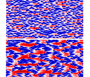
This subsection is devoted to a discussion of local time-averaged flow and its statistics. First, we need to settle the discussion of secondary flows opened in the previous subsection. To do so, in figure 8, time-averaged velocities at a  $y$–
$y$– $z$ plane crossing the centre of a patch for three ‘staggered’ cases are visualised. Note that to enhance statistical averaging, additional averaging is performed over all similar planes passing through centres of patches, therefore the contours within the roughness canopy bear no physical information (as roughness patches are not strictly identical). The purpose of this figure is to observe the presence of heterogeneity in mean flow above the roughness. For the streamwise velocity (figures 8a i,b i,c i), we deduct the horizontally averaged velocity
  $\langle \bar {u}\rangle$ from the local value
  $\bar {u}$ at each height. This facilitates observing the regions where flow is faster or slower than the mean, i.e. the high- and low-momentum pathways. Figures 8(a ii,b ii,c ii) clearly show an upwelling flow at the centre of a roughness patch, and a downwelling flow at its flanks, coinciding with low- and high-momentum pathways, respectively. Combined with the observed mean spanwise velocity, a clear swirl-like pattern can be identified in the time-averaged flow. This is similar to secondary motions of ‘ridge-type’ frequently reported in the past. Note that roughness-induced secondary motions have been reported previously mostly for purely spanwise heterogeneous roughness. The present results reveal that the same phenomenon can be induced by patchy roughness if the patches are placed in a regular (i.e. staggered) arrangement that can effectively mimic elongated regions of high and low roughness. Comparing different cases in figure 8, case STG50_1.4 is the one in which both upwelling motion and high/low-momentum pathways are the strongest (considering the maxima of
  $\bar {v}$ and
  $\bar {u}-\langle \bar {u} \rangle$ above the roughness crest). This is the case with the largest deviation from outer-layer similarity and dispersive stresses, both of which can be clearly linked to the secondary motions.

Figure 8. Mean normalised velocity on a plane at the centre of a patch at  $Re_\tau =180$: (a i,b i,c i)
  $(\bar {u} - \langle \bar {u} \rangle )/u_b$, (a ii,b ii,c ii)
  $\bar {v}/u_b$ and (a iii,b iii,c iii)
  $\bar {w}/u_b$, where
  $u_b$ is bulk velocity. Three cases are shown: (a) STG50_1.1, (b) STG50_1.4 and (c) STG50_2.1. In each case, flow over a single patch is shown. Dashed lines indicate the region occupied by roughness. The mean is calculated over time and multiple patches.
Mean local velocity profiles at the centres of rough and smooth patches are shown in figure 9 for three staggered samples with 50 % CR and different heterogeneity length scale values. Additionally, similar profiles are depicted for two cases in the NAT group; for these cases, the profiles are plotted for selected locations within smooth and rough patches, which are indicated by cross symbols in figure 3. In each plot, both smooth and rough profiles are normalised by the global friction velocity. Clearly, for the smallest  $\varLambda _P/\delta$, the velocity profiles collapse outside the region of direct roughness influence – the roughness sublayer, which extends up to
  $2k$–
$2k$– $3k$. As the size of the patches increases, the smooth and rough profiles lie farther apart, and each adapts to the new wall condition. At
  $\varLambda _P/\delta =8.5$, a change in the slope of the logarithmic profile from low to high is observed on the smooth profile (and vice versa for the rough profile). This demarcates the edge of the internal boundary layer, i.e. the region influenced by the new wall conditions. Note that in a channel, due to wall confinement, bulk velocity increases as the effective surface area decreases on rough patches, and consequently the velocity at the channel centre can be different on large smooth and rough patches.

Figure 9. Velocity profiles at the centre of smooth (solid line) and rough (dashed line) patches for five samples at  $Re_\tau =180$: (a) STG50_1.1, (b) STG50_4.2, (c) STG50_8.5, (d) NAT50_1.1, (e) NAT50_4.2. For the NAT cases, the locations of profiles are indicated by red crosses in figure 3. Viscous units are defined based on
  $u_{\tau,0}$.
In order to study the evolution of local flow and internal boundary layer in some depth, in figure 10, local wall shear stress as well as velocity and streamwise Reynolds stress profiles are plotted along the streamwise direction downstream of a rough patch for case STG50_8.5. The data are extracted for locations on two lines, one aligned with the centre of the patch (black), and one with an offset (blue), to shed light on any two-dimensional effects. Note that averaging over symmetry lines is used to enhance statistics. It is clearly observed that, affected by the recirculation zone past the last roughness elements, the local wall shear stress right behind the patch assumes smaller and even negative values at both locations. At about one  $\delta$ downstream, the shear stress reaches a plateau, which continues down to about one
  $\delta$ before the next patch, where it moderately drops again due to the diversion of the mean flow. Considering the local velocity profiles, despite the fact that the present Reynolds number does not provide a large logarithmic region, a clear change in the logarithmic slope of mean profiles is observed, starting at approximately 2
 $\delta$–3
 $\delta$, indicating formation and growth of the internal boundary layer. Note that the profiles with similar distance from a roughness patch (and not absolute
  $x$) are collapsed, which points towards a two-dimensional internal boundary layer. We also observe formation of a second peak in the Reynolds stress profiles (pointed at by arrows in figure 10d). These peaks form at the approximate wall distance of the internal boundary layer edge. Rouhi et al. (Reference Rouhi, Chung and Hutchins2019) observed similar second peaks in their DNS of flow past a rough-to-smooth step change.

Figure 10. (b) Local normalised wall shear stress, (c) time-averaged streamwise velocity, and (d) streamwise Reynolds stress on two streamwise lines downstream of a roughness patch for case STG50_8.5. The location for which the profiles are plotted in (c,d) are shown by cross symbols in (a) and by vertical dotted lines in (b). Here,  $\hat {x}$ denotes the streamwise distance from the edge of the immediately upstream patch (the horizontal lines in (a) indicate the respective
  $\hat {x}$-axes). A colour code is used to distinguish the two lines. Viscous units are defined based on
  $\tau _{w,0}^S$.
Finally, it can be insightful to compare mean shear stress over smooth and rough patches,  $\tau _{w,0}^S$ and
  $\tau _{w,0}^R$, for different patchy roughness. Figure 11 shows these values, normalised by the global mean, as a function of
  $\varLambda _P/\delta$ for all simulations. As expected, when
  $\varLambda _P/\delta$ grows and the equilibrium is approached, asymptotic convergence is observed as the equilibrium shear stresses over smooth and rough patches become independent of the patch geometry. The value of the asymptote, however, clearly depends on CR since the identity
  $(\tau _{w,0}^R/\tau _{w,0})\times \mathrm {CR}+(\tau _{w,0}^S/\tau _{w,0})\times (1-\mathrm {CR})=1$ must hold. Indeed, the specific wall shear stress distribution adjusts itself to the roughness CR. Finally, it is observed that at smaller values of
  $\varLambda _P/\delta$, the relative contribution of smooth parts of the wall to the total shear stress decreases (and vice versa for the rough part). This can be explained by the shear stress pattern downstream of a roughness patch, and the patch sheltering effect discussed with figure 10. It is fully expected to measure smaller mean shear stress on the smooth parts when patches are more closely packed since areas near a patch experience smaller local shear stress than those adequately far away. At the hypothetical limit of
  $\varLambda _P=0$, it is expected that
  $\tau _{w,0}^S/\tau _{w,0}$ becomes insignificant, hence
  $\tau _{w,0}^R/\tau _{w,0}\approx 1/\mathrm {CR}$, which agrees with the trend of the present data.

Figure 11. Mean wall shear stress for (a) smooth and (b) rough patches normalised with global wall shear stress  $\tau _{w,0}$ for
  $Re_\tau =180$. Symbols are similar to those in table 1.
3.4. Flow below the crest height
The focus in the previous subsection was mainly on the flow above roughness. The present subsection is devoted to a study of the flow at roughness crest and below it. We specifically attempt to shed light on the observation in § 3.1 that the computed values of  $C_f$ on some patchy roughness samples with small
  $\varLambda _P/\delta$ exceed that of homogeneous roughness at the same
  $\bar {\lambda }_f$. We begin the discussion with visualisations of the time-averaged flow on the
  $x$–
$x$– $z$ planes below the roughness crest. Expectedly, flow within a roughness patch (i.e. in the space between the roughness elements) is much slower than that outside. Apart from the patchy samples, we visualise the flow for two homogeneous cases in figure 12; the one with the same ‘mean’ frontal solidity (HOM_ML), and the one with the same frontal solidity as that of the patches (HOM_H). One can visually recognise that the flow below the roughness crest within the larger roughness patches closely resembles that of case HOM_H, when normalised with the bulk velocity. It can also be observed in figure 12 that the roughness elements at or near the patch perimeter are exposed to the larger velocity of the roughness-free region. When the patch is small, a larger portion of roughness elements is exposed to such high velocities, which obviously creates a larger drag force. This observation can be the key to explain why patchy roughness samples with small
  $\varLambda _P$ generate larger drag coefficients compared to other samples with similar overall numbers of elements. This effect is particularly pronounced when the patches are in a staggered arrangement, as in an irregular patch arrangement, different patches can shelter each other and behave rather as a larger patch.

Figure 12. Time-averaged streamwise velocity  $\bar {u}$ normalised with
  $u_b$ at 75 % of roughness height for selected samples. All samples are
  $12\delta \times 6\delta$. Samples are (a) HOM_ML, (b) HOM_H, (c) STG50_1.1, (d) STG50_4.2, (e) STG50_8.5, (f) NAT50_1.1 and (g) NAT50_4.2.
In order to quantify the observations described in the previous paragraph, in figure 13, we plot mean ‘intrinsic’ velocity within the patch, which is defined here as the mean velocity in the space between roughness elements within the area covered by patches – each patch is half an element diameter expanded to include the elements at the perimeter. It is clearly observed that larger patches result in smaller mean velocities within each patch. This is the velocity that the roughness elements are exposed to. Indeed, the velocity is smallest for the homogeneous sample HOM_H, which can be considered a roughness patch with an infinitely large patch size ( $\varLambda _P/\delta \rightarrow \infty$). For patchy roughness with finite
  $\varLambda _P/\delta$, the velocity departs further from that of HOM_H as the patch size decreases. Notably, the small patches in the STG group experience larger velocities than those in the NAT group, which is consistent with the comparative values of
  $C_f$.

Figure 13. Intrinsically averaged ‘patch’ velocity profiles below the roughness crest for all (a) STG50_xx and (b) RND/NAT50_xx cases at  $Re_\tau =180$ (the results at
  $Re_\tau =520$ are displayed in Appendix C). Colours and line patterns are identical to those in figure 6.
Finally, to shed further light on the previous observations, we consider the balance of forces within the flow. One can integrate the horizontally averaged momentum equation from centre of the channel to an arbitrary height  $y$ to yield the equation
 \begin{equation} ({-}P_x/\rho)\times(\delta-y)=\nu\,\frac{\mathrm{d}\langle\bar{u}\rangle}{\mathrm{d} y}-\langle\overline{u^\prime v^\prime}\rangle-\langle\tilde{u}\tilde{v}\rangle+F_D^y, \end{equation}
where terms on the right-hand side represent different contributions balancing the driving force of the mean pressure gradient on the left-hand side. The first, second and third terms on the right-hand side represent momentum transfer by viscous, Reynolds and dispersive shear stress, respectively, and  $F_D^y$ is the drag force exerted on the flow by all roughness elements between the the roughness crest and
  $y$.
$y$.
Different terms in (3.4) are depicted in figure 14 for three roughness samples with 50 % CR and different values of  $\varLambda _P/\lambda$. Clearly, far above the roughness crest, momentum transport is dominated by turbulence, and as a result, the contribution of Reynolds stresses is dominant, with contributions of viscous and dispersive stresses rapidly vanishing towards the centre of the channel. Remarkably, for the case with the smallest heterogeneity length scale (STG50_1.1), the dispersive stress makes the largest positive contribution, which is arguably a result of mean wall-normal velocity frequently changing direction on the windward and leeward sides of the patches. Our main interest is, however, the budget of forces below the roughness crest. This is the region where roughness drag force assumes non-zero values, and moreover, viscous stress makes a meaningful contribution. For obvious reasons, the viscous and roughness drag forces are the only terms with non-zero values at
  $y=0$. The ratio of these two terms at
  $y=0$ indicates the relative contribution to
  $\tau _{w,0}$ of viscous drag on the bottom wall, and drag on the roughness elements. The present results clearly demonstrate that at smaller values of
  $\varLambda _P/\delta$, the drag force on roughness elements makes a larger contribution to the total drag; as
  $\varLambda _P/\delta$ grows, it loses more share to the viscous shear stress. It must be kept in mind that the total numbers of roughness elements in all cases shown in figure 14 are the same, which means that, on average, a roughness element in a small patch stands a larger drag force. This is in line, on the one hand, with the above discussion on the effect of patch size on roughness drag, and on the other hand, with the observation in figure 11 that
  $\tau _{w,0}^R/\tau _{w,0}$ increases as
  $\varLambda _P/\delta$ decreases.

Figure 14. Budget of different forces in (3.4) for three STG cases with increasing  $\varLambda _P/\delta$ at
  $Re_\tau =180$. All forces are normalised by
  $u^2_{\tau,0}$. The dashed line indicates the sum of all forces, i.e.
  $(-({P_x}/{\tau _{w,0}}))\times (\delta -y)$. (It crosses unity at
  $y=k_{md}$ by definition of
  $\tau _{w,0}$.) Samples are (a) STG50_1.1, (b) STG50_4.2 and (c) STG50_8.5.
4. Conclusions
Direct numerical simulations of turbulent flow in plane channels with heterogeneous (patchy) and homogeneous roughness are carried out, in which roughness patches are generated by distributing discrete roughness elements approximately resembling sessile barnacles in maritime applications. Both regular and random patch arrangements are studied, and the heterogeneity length scale  $\varLambda _P$ and coverage ratio (CR) of roughness are varied. The main purpose is to shed light on whether and how the global skin-friction coefficient
  $C_f$ of patchy roughness can be determined if a correlation for corresponding homogeneous roughness at the same Reynolds number is in hand. Specifically, we compare the
  $C_f$ values of the patchy roughness at each CR with two limiting values:
  $C_f$ of homogeneous roughness with the same ‘mean’ properties, and the area-weighted mean of homogeneous
  $C_f$ based on local properties. When
  $\varLambda _P$ is of the order of channel half-height
  $\delta$, we observe that the global
  $C_f$ is close to the first limiting case, indicating that the flow may perceive roughness similar to a homogeneous one. At this limit, however, a rather large scatter is observed, dependent on the patch arrangement; for a regular (staggered) arrangement,
  $C_f$ can overshoot that of the first limiting value. This can be attributed to exposure of roughness elements to the large velocities outside the patch, hence producing large drag forces. Indeed, an analysis of force balance within the roughness canopy shows a larger drag force on roughness elements when the roughness patch is smaller.
As  $\varLambda _P/\delta$ grows, the value of the friction coefficient moves towards the second limiting value, and the arrangement-dependent scatter reduces. Expectedly, at large
  $\varLambda _P/\delta$,
  $C_f$ asymptotically approaches a constant ‘equilibrium’ value. Our observation shows that a mere order of magnitude separation between
  $\varLambda _P$ and
  $\delta$ is sufficient for
  $C_f$ to be well approximated by the equilibrium value. This observation motivated suggesting a correlation for the friction coefficient of patchy roughness normalised by the two limiting cases as a function of
  $\varLambda _P/\delta$ (3.2). The correlation includes three fitting constants, which can be (weak) functions of patch arrangement and CR. A key question is whether the
  $\delta$-scaling is valid across a wide range of Reynolds numbers. While the current results in the range
  $180\leq Re_\tau \leq 520$ and the discussed literature on streamwise heterogeneous roughness suggest a moderate effect of Reynolds number at most, experiments at (much) larger Reynolds numbers are required to settle this question. Practically, a minor Reynolds number dependence can be accommodated in the proposed correlation form by making the constants functions of Reynolds number.
Overall, our results show the possibility of predicting drag on heterogeneous roughness based on available correlations on homogeneous roughness. This should, however, go beyond a simple use of those correlations with ‘mean’ roughness properties measured over the entire surface area (i.e. the first limiting case in the present study, represented by (1.3)). Indeed, such a simplistic practice can be misleading in many cases. For example, as shown by Sarakinos & Busse (Reference Sarakinos and Busse2022),  $k_s$ for patchy roughness decreases with skewness, which is in contrast with the generally accepted trend, and the result of the fact that the values of skewness have been calculated based on the entire plan area by those authors.
We also study global and local time-averaged velocities, and certain second-order flow statistics. Notably, for a staggered patch arrangement and at a narrow range of patch distance (in the vicinity of  $\delta$), roughness-induced secondary flows are observed when the time-averaged velocity is concerned. While these flows are widely reported in the literature for purely spanwise roughness heterogeneity, the present observation indicates that patchy roughness can induce the same effect if it mimics high- and low-roughness strips due to a regular arrangement. The secondary motions are also shown to be linked to deviation from outer layer similarity of mean velocity profiles as well as considerable non-zero values of dispersive stress beyond the roughness sublayer. It is arguable that secondary motions partly contribute to the scatter of
  $C_f$ values at low
  $\varLambda _P/\delta$, but their effect is deemed to be of secondary importance. We also identified the possible development of an internal boundary layer downstream of the roughness patches, and a corresponding second peak in streamwise Reynolds stress profiles. Further investigation of this issue, however, requires larger Reynolds numbers to support a clear inner–outer scale separation.
The present work provides the basis for a framework to estimate the drag on patchy roughness, with obvious practical implications. It is, however, important to investigate at least a few important effects before generalising the results. Most importantly, since the Reynolds numbers in the real-world applications associated with this problem are far beyond the reach of the DNS methodology, experiments at high Reynolds number are essential to establish any Reynolds number effects. Furthermore, the present study considers a simplistic roughness type consisting of mono-disperse elements. While this choice facilitated isolating the heterogeneous effects in the present work, real-world roughness often features more complex topographies that cannot be parametrised by a single parameter. Arguably, the choice of predictive roughness parameters ( $\boldsymbol {X}$ in (1.1)) is a factor affecting the patchy roughness correlation relying on it. While there is no lack of discussion on the choice of predictive parameters in the literature, the focus has always been on homogeneous roughness. Taking that into account, we call for alternative assessments of homogeneous roughness correlations in terms of whether they can support a convenient heterogeneous roughness correlation (i.e. (3.2)). Finally, future studies on developing boundary layers – as opposed to fully developed channel flow – will be essential to complete the picture.
Funding
P.F. gratefully acknowledges support from Aarhus University Research Foundation (grant no. AUFF-F-2020-7-9).
Declaration of interests
The authors report no conflict of interest.
Data availability
All data are available upon request.
Appendix A. Coefficient  $C_f^{eq}$ for streamwise heterogeneous roughness

This appendix aims to clarify the physical meaning of the mean homogeneous friction coefficient  $\overline {C_f^{hom}}$ and its link to the equilibrium friction coefficient – an issue frequently mentioned in the body of the paper. Consider a plane channel with purely streamwise roughness heterogeneity, i.e. patches of smooth and rough wall elongated indefinitely in the spanwise direction. We assume that patches are large enough for the flow on each patch to reach equilibrium, in which case, the friction coefficients over rough and smooth patches converge to that of a fully developed flow over a homogeneous rough wall (
 $C_{f,{rough}}^{{hom}}$) or smooth wall (
 $C_{f,{smooth}}^{{hom}}$). If the patches are large enough for the edge effects to vanish, then the above homogeneous friction coefficients determine the drag force on the smooth and rough parts of the wall. As a result, the total drag force becomes
 \begin{equation} F=F_{{smooth}}+F_{{rough}}=\frac{\rho}{2} \left(C_{f,{smooth}}^{{hom}}\,u_{b,{smooth}}^2\,A_{{smooth}}+ C_{f,{rough}}^{{hom}}\,u_{b,{rough}}^2\,A_{{rough}}\right), \end{equation}
where  $A$ denotes the plan wall area. In an ideal case when the change of cross-section due to roughness can be neglected (which is, for instance, not the case for the geometries studied in the present work), continuity requires bulk velocity to be independent of the streamwise direction, hence
  $u_{b,{smooth}}=u_{b,{rough}}=u_{b}$. Dividing (A1) by
  $({\rho }/{2}) u_b^2\,A_{total}$, and considering the definitions of global friction coefficient
  $C_f$ and CR, one obtains
 \begin{equation}
C_f=C_{f,{smooth}}^{hom}\times
(1-\mathrm{CR})+C_{f,{rough}}^{hom}\times
\mathrm{CR}.
\end{equation}
\begin{equation}
C_f=C_{f,{smooth}}^{hom}\times
(1-\mathrm{CR})+C_{f,{rough}}^{hom}\times
\mathrm{CR}.
\end{equation}
The  $C_f$ on the left-hand side of the above equation is the equilibrium friction coefficient. The right-hand side is the area-weighted average of
  $C_f$ on smooth and rough walls under fully developed homogeneous conditions. Therefore, (A2) in generalised form is equivalent to
  $C_f^{eq}=\overline {C_f^{hom}}$. Note that the above derivation is valid only for streamwise heterogeneous roughness with the outlined idealised assumptions (edge effects and variation of cross-section both negligible). For the spanwise case, for example, Neuhauser et al. (Reference Neuhauser, Schäfer, Gatti and Frohnapfel2022) derived
  $1/\sqrt {C_f^{eq}}=\overline {1/\sqrt {C_f^{hom}}}$. In the general case, obtaining an expression for
  $C_f^{eq}$ is not straightforward and outside the scope of the present work.
Appendix B. Further characterisation of homogeneous samples
While not a central element of the present work, it can provide further insight to characterise the homogeneous roughness cases discussed extensively in the paper, and their flow regime (transitional versus fully rough). We avoid a discussion of the fully rough regime for the heterogeneous roughness cases as its existence is an open issue in the literature (Gatti et al. Reference Gatti, von Deyn, Forooghi and Frohnapfel2020; Frohnapfel et al. Reference Frohnapfel, von Deyn, Yang, Neuhauser, Stroh, Örlü and Gatti2024) and far from the scope of the present work.
We characterise roughness samples HOM_ML and HOM_H by running simulations at four Reynolds numbers between  $Re_\tau =180$ and
  $Re_\tau =750$. To minimise the computational cost, we run these simulations in channels with reduced domain sizes following the approach of Chung et al. (Reference Chung, Chan, MacDonald, Hutchins and Ooi2015) and MacDonald et al. (Reference MacDonald, Chung, Hutchins, Chan, Ooi and García-Mayoral2017). The sizes of the reduced-domain channels in the present work are larger than the minimum proposed by those works. Details of these simulations are shown in table 3. Note that in reduced-domain simulations, the flow is physical up to wall distance
  $y_{res}^+=0.4L_z^+$ as the reduced channel span does not allow resolving large structures beyond this height (Chung et al. Reference Chung, Chan, MacDonald, Hutchins and Ooi2015; MacDonald et al. Reference MacDonald, Chung, Hutchins, Chan, Ooi and García-Mayoral2017). Subsequently, in all the present cases,
  $L_z$ is chosen so that the roughness tip is much smaller than
  $y_{res}$ (about one-fifth of it).
Table 3. Domain size and grid resolution information for performed minimal DNS cases, where  $L_x,L_z$ denote domain sizes in streamwise and spanwise directions, and
  $N_x, N_y, N_z$ denote numbers of grid points. The grid is uniform in the streamwise and spanwise directions. Also,
  $\Delta y^+_c$ and
  $\Delta y^+_0$ denote wall-normal resolution at the centre of the channel and at the bottom walls, respectively.

The computed values of the roughness function at different Reynolds numbers are plotted in figure 15 against the inner-scaled values of equivalent sand-grain roughness for the respective roughness. For each roughness,  $k_s$ is obtained by scaling the physical roughness size
  $k$ until its data collapse into the fully rough asymptote for uniform sand grains (Nikuradse Reference Nikuradse1933). The scaling factor
  $k_r$ is obtained to be 2.9 and 2.8 for the HOM_ML and HOM_H cases, respectively, meaning that
  $k_s=2.9k$ for the former, and
  $k_s=2.8k$ for the latter. Importantly, the fully rough regime for both HOM_ML and HOM_H seems to have already been reached at
  $k_s^+\approx 100$ (
 $Re_\tau =395$). Moreover, these roughness samples show a ‘Nikuradse-type’ behaviour in the transitionally rough regime, which is the expected behaviour considering the identical sizes of the roughness elements.

Figure 15. Roughness function as a function of inner-scaled equivalent sand-grain roughness ( $k_s^+=k_r\times k^+$) for roughness samples HOM_ML and HOM_H compared to uniform sand-grain roughness (Nikuradse Reference Nikuradse1933) and industrial pipe roughness (Moody Reference Moody1944). The solid line shows the fully rough asymptote.
Finally, in order to calculate  $u_b$, and subsequently
  $C_f=2/{u_b^+}^2$, from the mean velocity profiles computed in the reduced-domain simulations, we follow the idea proposed by Rouhi et al. (Reference Rouhi, Endrikat, Modesti, Sandberg, Oda, Tanimoto, Hutchins and Chung2022, Reference Rouhi, Fu, Chandran, Zampiron, Smits and Marusic2023) that the unresolved part of the profile beyond
  $y_{res}$ can be replaced by that of a ‘physical’ profile at a similar Reynolds number and flow type. This will ensure that for the calculation of
  $u_b$, correct logarithmic and wake profiles are integrated above
  $y_{res}$. We use the DNS of del Álamo & Jiménez (Reference del Álamo and Jiménez2003) in a smooth plane channel at
  $Re_\tau \approx 550$ as the reference physical profile. Note that in the case of rough reduced-domain channels, a
  $\Delta U^+$ shift should be applied to the reference smooth profile so the profiles match at
  $y_{res}$.
Appendix C. Flow profiles at $Re_{\tau }=520$

A limited number of heterogeneous roughness cases have been run at larger Reynolds number  $Re_{\tau }=520$. To avoid prolonging the body of paper, first- and second-order statistics corresponding to those shown previously for
  $Re_\tau =180$ are shown in this appendix. These results are shown in figures 16–18. No homogeneous and smooth profiles are shown in these figures as the homogeneous and smooth cases at
  $Re_\tau =520$ are simulated in reduced-domain simulations, which delivers non-physical results above
  $y_{res})$. The exception is figure 18, in which the profiles are shown only up to the roughness crest, which is well below
  $y_{res})$.

Figure 16. Mean velocity profiles, with (b) in defect form, for STG50_xx cases at  $Re_\tau =520$. Line colours follow the symbol colours in table 1.

Figure 17. Streamwise (a) Reynolds and (b) dispersive stresses for STG50_xx cases at  $Re_\tau =520$. Line colours and styles are similar to those in figure 16.

Figure 18. Intrinsic velocity below the roughness crest for STG50_xx cases at  $Re_\tau =520$. Line colours and styles are similar to those in figure 16. The dashed line represents the homogeneous roughness HOM_H.


 Open access