


1. Introduction
While a large body of research on how a smooth-wall turbulent boundary layer (TBL) responds to different pressure gradients (PGs) has been well documented in the literature, there are only a few studies on how PGs can affect rough-wall-bounded flows (Perry & Joubert Reference Perry and Joubert1963; Aubertine, Eaton & Song Reference Aubertine, Eaton and Song2004; Pailhas, Touvet & Aupoix Reference Pailhas, Touvet and Aupoix2008). It is well documented that the roughness can disrupt the mechanism of self-sustaining turbulence production in zero pressure gradient (ZPG) TBLs (Krogstad & Antonia Reference Krogstad and Antonia1994; Jiménez Reference Jiménez2004; Djenidi et al. Reference Djenidi, Antonia, Amielh and Anselmet2008). This raises two questions: (i) what is the response of a rough-wall TBL to PGs, and (ii) how does this response differ from that of a smooth-wall TBL? Answering these questions is not only of fundamental importance in fluid mechanics, but is also of significance from an engineering point of view, e.g. airflow in nozzles or over turbine blades, wind flows over hillsides and underwater flow on a fouled surface of a ship hull. Information in this research area is somewhat scanty and fragmented (Dvorak Reference Dvorak1969; Durbin et al. Reference Durbin, Medic, Seo, Eaton and Song2001; Cal et al. Reference Cal, Brzek, Johansson and Castillo2008; Piomelli & Yuan Reference Piomelli and Yuan2013), hindering our ability to quantify and, quite importantly, predict the statistical behaviour of rough-wall TBLs subjected to PGs.
A survey of the literature reveals only a few studies dealing with rough-wall TBLs under adverse pressure gradient (APG). Using high-resolution laser Doppler anemometry, Song & Eaton (Reference Song and Eaton2002) studied the effects of wall roughness on flow separation over a ramp at Reynolds number ( $Re_\theta =U_1\theta /\nu$, where
  $\theta$ is the momentum thickness,
  $U_1$ is the free stream velocity and
  $\nu$ is the kinematic viscosity) of up to 3000. Their results showed that the separation starts earlier in rough-wall TBLs as compared with that in smooth flows, suggesting a larger mean momentum deficit in the vicinity of the roughness elements. It was also found that the reattachment is delayed for the rough case and thus the separation bubble becomes thicker. Similar outcomes can be found in the measurements of Aubertine et al. (Reference Aubertine, Eaton and Song2004) and Cao & Tamura (Reference Cao and Tamura2006). An APG increases the thickness of the boundary layer and the region influenced by length scales associated with the roughness element. Tay, Kuhn & Tachie (Reference Tay, Kuhn and Tachie2009a) showed that at
  $900 \leq Re_\theta \leq 3000$, the turbulence level and Reynolds shear stress in the proximity of the roughness elements are increased when compared with a smooth-wall TBL. Their results were supported by Wu & Piomelli (Reference Wu and Piomelli2018), who further demonstrated that when an APG is imposed, at
  $Re_\theta = 2500$, the flow within the wake region of the roughness elements alters the intermittency of the near-wall turbulence. It was also shown that in the APG case, the flow moves slower within the wake of the roughness elements than in the ZPG case. Hot-wire measurements conducted by Shin & Song (Reference Shin and Song2015b) showed that at
  $Re_\theta \approx 3600$, an APG weakens the effect of roughness on vortical structures near the peak of the roughness elements and reduces the kinetic energy more in a smooth-wall TBL.
A study of a rough-wall TBL under favourable pressure gradient (FPG) at  $Re_\theta \leq 3500$ shows that the streamwise root-mean-square velocity in the regions close to the roughness elements is reduced as compared with the unaccelerated data while the turbulence structures are less isotropic in the inner region of the boundary layer (Coleman, Moffat & Kays Reference Coleman, Moffat and Kays1977). The combined effect of FPG and roughness on the TBL has also been investigated in an asymmetric converging channel in which the flow evolved over straight and inclined transverse ribs attached to the top and bottom walls (Tachie & Shah Reference Tachie and Shah2008). It was observed that the turbulence level is strongly dependent on the roughness orientation. For straight ribs, the effects of roughness in the inner wall region outweigh the PG influence. However, FPG reduces the Reynolds normal stresses in the outer region. On the other hand, when the ribs are inclined the effect of FPG is stronger in the trailing edge of the roughness than at the leading edge of the rib. This results in a 50 % reduction in skin friction. This is in contrast to the findings of Tay, Kuhn & Tachie (Reference Tay, Kuhn and Tachie2009b) in a low-Reynolds-number TBL (
 $Re_\theta < 2500$) over a two-dimensional asymmetric converging-channel rough wall. Their particle image velocimetry results revealed that, compared with the canonical TBL, both the friction velocity and skin friction coefficient are increased, while the turbulent intensities and Reynolds shear stress significantly decrease with increasing FPG. This is supported by Cal et al. (Reference Cal, Brzek, Johansson and Castillo2009), who measured the wall shear stress using the full integrated momentum equation at
  $Re_\theta < 5000$. They found that in the fully rough regime and regardless of
  $Re$, FPG increases the friction drag. It was also shown that turbulence production decreases with increasing FPG strength, even though it was observed that surface roughness tends to increase the energy production when compared with a smooth wall. At lower
  $Re_\theta$ (< 2700), Shin & Song (Reference Shin and Song2015a) showed that due to strengthened vortices and associated shear stress in the accelerated flows over a rough surface, increasing mean velocity defect in the FPG case is stronger than in the ZPG one. It was also evident that FPG generates extra turbulence energy in rough TBLs resulting in an increased overall turbulent kinetic energy and also friction coefficient.
From modelling and prediction/estimation viewpoints, it is of great interest to determine whether a TBL can be in a universal or self-preservation (SP) state in a wide range of Reynolds numbers impossible to achieve in a laboratory. For example, SP allows determination of adequate sets of scaling length and scaling velocity which can be used to interpret data in a meaningful manner. The concept of SP implies that the equations governing the flow admit similarity solutions based on a unique scale of length and velocity. In the literature, SP refers to an ‘equilibrium’ state, where the local rates of turbulent kinetic energy production and dissipation are so large that the turbulent motions are independent of the other flow conditions (Bradshaw Reference Bradshaw1967; Skaare & Krogstad Reference Skaare and Krogstad1994; Bobke et al. Reference Bobke, Vinuesa, Örlü and Schlatter2017; Vila et al. Reference Vila, Vinuesa, Discetti, Ianiro, Schlatter and Örlü2020). In smooth-wall TBL studies, friction velocity ( $U_\tau$) and
  $\nu /U_\tau$ are used as inner velocity and length scales, respectively, while
  $U_1$ and the boundary layer thickness (
 $\delta$) are used as outer velocity and length scales, respectively. In the case of rough-wall TBL in a fully rough regime, where
  $U_\tau /U_1 = \sqrt {C_f/2}$ (
 $C_f$ is the skin friction coefficient) is constant, one can use either
  $U_\tau$ or
  $U_1$ as velocity scaling (Djenidi, Talluru & Antonia Reference Djenidi, Talluru and Antonia2018), while the appropriate length scale is
  $\delta$. The reason why a smooth-wall TBL requires two scaling velocities is due to the existence of two regions: a viscous-dominated sublayer that imposes its own scaling and an outer region where the effect of viscosity is negligible. In a fully rough TBL, there is no viscous-dominated sublayer. This explains why a fully rough TBL is in complete SP (i.e. SP across the entire boundary layer thickness) (Rotta Reference Rotta1962; Talluru et al. Reference Talluru, Djenidi, Kamruzzaman and Antonia2016). Despite the large body of work on outer similarity studies of both smooth-wall and rough-wall TBLs (Townsend Reference Townsend1980; George & Castillo Reference George and Castillo1997; Castillo & George Reference Castillo and George2001; Jones, Nickels & Marusic Reference Jones, Nickels and Marusic2008), no rigorous SP analyses have been conducted on rough-wall TBLs under different PGs. So far, Brzek (Reference Brzek2007) and Cal et al. (Reference Cal, Brzek, Johansson and Castillo2009) showed that using
  $U_\tau$ to normalize the mean velocity profiles of a rough-wall TBL subjected to FPG leads to an underestimate of the actual effect of the PG on the velocity and hides the roughness impacts in the outer region of the boundary layer, while free-stream velocity scaling is more susceptible to the surface roughness. Due to the challenges associated with estimating
  $U_\tau$ in rough-wall TBLs subjected to PGs (Perry, Schofield & Joubert Reference Perry, Schofield and Joubert1969), Chao, Castillo & Turan (Reference Chao, Castillo and Turan2007) used the free-stream velocity
  $U_1$ or the mixed outer scale (
 ${U_1\delta ^{*}/\delta }$, where
  $\delta ^{*}$ is the displacement thickness), suggested by Zagarola & Smits (Reference Zagarola and Smits1998), and showed that they are more appropriate scaling parameters.
The above brief review of accelerated or decelerated rough-wall TBLs at relatively low Reynolds numbers shows that our current knowledge of the dynamic behaviour of rough-wall TBLs subjected to external PGs is, compared with that of smooth-wall TBLs under PGs, limited; there is virtually no study on SP of a rough-wall TBL under PG, for example. The present study, which in a sense follows and extends the previous study is an attempt at helping expand this knowledge by studying rough-wall TBLs subjected to different PGs for different Reynolds numbers. The study is primarily aimed at addressing, at least partially, the following questions:
(i) How does a fully rough TBL react to different PGs over a wide range of
 $Re$?
$Re$?(ii) Is the SP state of a rough-wall TBL ‘disturbed’ or maintained when PGs are applied?
(iii) Are the energy-containing motions in rough-wall TBLs affected differently by PGs?

Addressing these questions should provide an insight into the underlying physics of rough-wall TBLs subjected to PGs, which can be exploited for the development of effective control strategies.
2. Experimental set-up and procedures
The experiments are conducted in the boundary layer wind tunnel at the University of Newcastle. The test section of this open-return blower wind tunnel is 4 m long, 0.9 m wide and 0.16 m high (further details of the facility can be found in Kamruzzaman et al. (Reference Kamruzzaman, Djenidi, Antonia and Talluru2015) and Djenidi, Kamruzzaman & Dostal (Reference Djenidi, Kamruzzaman and Dostal2019a)). Before any PG is introduced, the ZPG boundary layer evolves over more than 15 boundary layer thicknesses which is sufficiently upstream of the onset of the PG (Sreenivasan Reference Sreenivasan1989). At the inlet, the flow is tripped by a 100 mm strip of coarse-grade P40 sandpaper, spanning the width of the test section to trigger the TBL and ensure that SP is reached before the PG is applied. The inlet ZPG section is followed by a 3 m test section with an adjustable ceiling that consists of two rectangular panels each of dimensions 1.75 m in length and 0.9 m in width. The PG is achieved by adjusting the height of these panels and varying the bleeding gap between them. The streamwise evolution of the boundary layer thickness on both rough surface and ceiling is measured to ensure that at no location do the boundary layers not affect each other. Variation of the pressure coefficient with streamwise direction  $x$ is estimated as follows and is shown in figure 1 for different streamwise locations:
 \begin{equation} C_p=\frac{p_1-p_i}{\frac{1}{2}\rho{U_1}^{2}}, \end{equation}
where  $p_1$ is the local static pressure measured by wall tappings,
  $p_i$ is the static pressure at the beginning of the ZPG section and
  $\rho$ is the density of air. Figure 1 shows how the pressure coefficient varies in the streamwise direction for different PGs. The PG is characterized by the following Clauser PG parameter (
 $\beta$) or acceleration parameter (
 $K$):
$K$):
 \begin{equation} \beta = \frac{\delta^{*}}{\tau_w}\frac{\partial {p_1}}{\partial {x}} ,\quad K = \frac{\nu}{U_1^{2}}\frac{\partial {U_1}}{\partial {x}}, \end{equation}
where  $\tau _w$ is the wall shear stress. In this study, the rough-wall TBLs are subjected to a narrow range of PGs where
  $\beta$ varies from 0.72 to
  $-0.12$, i.e. from APG to FPG.

Figure 1. Pressure coefficient  $C_P (x)$ along the plate for APG (blue symbols) and FPG (red symbols) cases. See table 1 for symbols.
The rough TBL develops over a rough surface consisting of cylindrical rods arranged periodically and spanning the entire width of the test section. The rods with a nominal diameter of 1.6 mm (with a standard deviation of 0.1 mm) are positioned at a streamwise spacing to roughness height ( $k$) ratio of 15. The main challenge in rough TBL studies is associated with an accurate calculation of the friction velocity,
  $U_\tau =\sqrt {\tau _w/\rho }$, as most of the scaling laws rely on this value. While a number of indirect techniques such as Clauser chart and power-law methods are available to determine this value over smooth surfaces, none are universally accepted for fully rough TBLs due to their additional estimated parameters such as the fictitious origin for the mean velocity profile. In this study, we measure the friction velocity and the coefficient of PG
  $C_{D, p}$ by integrating the pressure distribution around the roughness element (the method is described in detail in Kamruzzaman et al. (Reference Kamruzzaman, Talluru, Djenidi and Antonia2014)). The boundary layer thickness is also determined from the defect chart method suggested by Djenidi, Talluru & Antonia (Reference Djenidi, Talluru and Antonia2019b) and also the modified Coles law of the wall/wake fit to the mean velocity (Perry, Marusic & Jones Reference Perry, Marusic and Jones2002). All velocity measurements are taken at the mid-point of two adjacently spaced roughness elements at five streamwise stations for two different inlet velocities,
  $U_{i}$ (figure 2). Based on the method proposed by Jackson (Reference Jackson1981), the
  $y$ origin is taken to be the plane at a distance of
  $d_0\approx$ 0.4
 $k$. In order to achieve high-fidelity data over long time scales, and investigate mean statistics, a single Dantec 55P15 hot-wire was mounted to a fine threaded traversing system with a resolution of 1
  $\mathrm {\mu }$m in positioning close to the wall. A wire diameter (
 $d$) of 2.5
  $\mathrm {\mu }$m with an etched length (
 $l_{HW}$) of 0.4–0.6 mm is used to achieve
  $l_{HW}^{+} \lesssim 54$, an
  $l_{HW}/d$ ratio of around 200, as recommended by Ligrani & Bradshaw (Reference Ligrani and Bradshaw1987) and Hutchins et al. (Reference Hutchins, Nickels, Marusic and Chong2009). However, we showed previously (Ghanadi & Djenidi Reference Ghanadi and Djenidi2021b) that for the present rough wall there is no attenuation associated with a spatial resolution for
  $l_{HW}^{+}$ up to 160. The wire is operated with an in-house constant-temperature circuit at an overheat ratio of 1.8. This value is minimized owing to the thermal wall effects, which can become important when multiple thermal sensors are located in close proximity. In order to converge statistics at all scales of motion in the spectra, the total length in seconds of the velocity sample is 180, sampled at up to 70 kHz. A temperature anemometer (BAT-10 thermocouple, Physitemp) is also installed in the free stream and continuously monitored with an accuracy of
  $\pm 0.1\,^{\circ }$C throughout the course of the experiment. Table 1 shows the flow parameters for the study. Two inlet velocities are used:
  $U_{i,l}=10\,{\rm m}\,{\rm s}^{-1}$ and
  $U_{i,h}=20\,{\rm m}\,{\rm s}^{-1}$. Note that in the case of FPG,
  $U_i$ is slightly reduced in comparison with the ZPG and APG cases.

Figure 2. A schematic of the experimental set-up. The inset shows the spacing between two consecutive roughness elements.
Table 1. Flow parameters for rough-wall TBLs under different PGs: ZPG (black), APG (blue) and FPG (red). The table is separated into two sections with different inlet velocities:  $U_{i,l}=10$ m s
 $^{-1}$ (top section);
  $U_{i,h}= 20$ m s
 $^{-1}$ (bottom section). The symbols listed here are used consistently throughout the paper.

3. Results
3.1. Mean and turbulence statistics
The mean streamwise velocity distributions normalized by the wall units (i.e.  $U_\tau$ and
  $\nu /U_\tau$) at different
  $x$ locations (figure 3) reveal that the effects of PGs are similar for both smooth-wall (not shown here) and rough-wall TBLs in the outer region. There is an upward shift when APG is applied and a downward shift when FPG is applied, which is consistent with deceleration and acceleration, respectively. Similar flow behaviours under PGs are also observed in previous smooth-wall studies at various
  $Re$ (Spalart & Watmuff Reference Spalart and Watmuff1993; Harun et al. Reference Harun, Monty, Mathis and Marusic2013; Vila et al. Reference Vila, Vinuesa, Discetti, Ianiro, Schlatter and Örlü2020). It is observed though that at the stations closer to the inlet (I to III) (figure 3b), the effect of PGs for the rough-wall TBL penetrates in the logarithmic region
  $200\leq y^{+} \leq 800$; this influence is, however, modulated by the Reynolds number which shows a less impacted logarithmic region.

Figure 3. Inner-normalized mean streamwise velocity profiles for different PGs: (a)  $U_{i,l}$; (b)
  $U_{i,h}$. Dashed black lines have a slope of 1/0.4. See table 1 for symbols.
In the present study, we carry out a SP analysis for the rough-wall TBL with PGs. The equation for the streamwise mean velocity,  $U$, in the case of the fully rough-wall TBL, where there is no viscous sublayer (Schultz & Flack Reference Schultz and Flack2007; Krogstad & Efros Reference Krogstad and Efros2012), is
 $$\begin{gather} \langle \bar{U}\rangle \frac{\partial \langle \bar{U}\rangle}{\partial x}+\langle \bar{V}\rangle\frac{\partial \langle \bar{U}\rangle}{\partial y}={-}\frac{\partial (\langle \overline{{u^{\prime}}{v^{\prime}}}\rangle+(\langle \overline{u^{\prime\prime}}\cdot\overline{v^{\prime\prime}}\rangle)}{\partial y} -\frac{\partial(\langle \overline{{u^{\prime}}^{2}}\rangle+\langle \overline{{u^{\prime\prime}}^{2}}\rangle)-(\langle \overline{{v^{\prime}}^{2}}\rangle+\langle \overline{{v^{\prime\prime}}^{2}}\rangle)}{\partial x}\nonumber\\ -\frac{1}{\rho}\frac{\mathrm{d}\langle p\rangle}{\mathrm{d}\kern0.06em x}+F, \end{gather}$$
where  $V$ is the mean velocity component in
  $y$, the direction normal to the wall, and
  $u$ and
  $v$ are the
  $x$ and
  $y$ components of the velocity fluctuations. The time and spatial fluctuating velocity components are denoted by a prime and double prime, respectively. An overbar denotes the time-averaged quantities. Note that a spatial averaging operation
  $\langle \,\rangle$ over a thin horizontal slap is also applied in (3.1) which allows accounting for the heterogeneity of the roughness elements (see Raupach, Antonia & Rajagopalan (Reference Raupach, Antonia and Rajagopalan1991) and Finnigan (Reference Finnigan2000) for more details). As the flow is irrotational with a constant total head, the PG can be written as
 \begin{equation} \frac{1}{\rho}\frac{\mathrm{d}p_1}{\mathrm{d}\kern0.06em x}={-}U_1\frac{\mathrm{d}U_1}{\mathrm{d}\kern0.06em x} \end{equation}
and the streamwise component of form drag  $F$ can be expressed as (see Raupach et al. (Reference Raupach, Antonia and Rajagopalan1991) for further details)
 \begin{equation} F=\frac{C_d}{k}{{\langle \bar{U}\rangle}^{2}}, \end{equation}
where  $C_d$ is the drag coefficient. Following Townsend (Reference Townsend1980) and George (Reference George1995), we assume the following SP forms for the various quantities in (3.1):
 \begin{gather} U_1-\langle \bar{U}\rangle=U_0f(\eta), \end{gather}
 \begin{gather} \langle \overline{{u^{\prime}}{v^{\prime}}}\rangle+\langle \overline{u^{\prime\prime}}\cdot\overline{v^{\prime\prime}}\rangle=U_{uv}^{2}g_{uv}(\eta), \end{gather}
 \begin{gather} \langle \overline{{u^{\prime}}^{2}}\rangle+\langle \overline{{u^{\prime\prime}}^{2}}\rangle=U_{u}^{2}g_u(\eta), \end{gather}
 \begin{gather} \langle \overline{{v^{\prime}}^{2}}\rangle+\langle \overline{{v^{\prime\prime}}^{2}}\rangle=U_{v}^{2}g_v(\eta), \end{gather}
where  $\eta =y/l$, and
  $l$ is a length scale;
  $U_0$,
  $U_u$,
  $U_v$ and
  $U_{uv}$ are velocity scales and not necessarily equal. The unknown functions
  $f$,
$f$,  $g_{uv}$,
  $g_u$ and
  $g_v$ are functions of
  $\eta$. Substituting these SP distributions in (3.1), using the continuity equation, then multiplying by
  $l/U_{uv}^{2}$ yield after some trivial manipulations
 \begin{align} &-\left[\frac{U_1 l}{{U_{uv}}^{2}}\frac{\mathrm{d}U_{0}}{\mathrm{d}\kern0.06em x}+\frac{U_0 l }{{U_{uv}}^{2}}\frac{\mathrm{d}U_1}{\mathrm{d}\kern0.06em x}\right]f+\frac{U_0 l }{U_{uv}^{2}}\frac{\mathrm{d}U_{0}}{\mathrm{d}\kern0.06em x}{f^{2}}+\left[\frac{U_1 U_0}{U_{uv}^{2}}\frac{\mathrm{d}l}{\mathrm{d}\kern0.06em x}-\frac{U_0 l}{U_{uv}^{2}}\frac{\mathrm{d}U_1}{\mathrm{d}\kern0.06em x}\right]\eta f'+g'_{uv}\nonumber\\ &\qquad -\left[\frac{U_0 l}{U_{uv}^{2}}\frac{\mathrm{d}U_{0}}{\mathrm{d}\kern0.06em x}+\frac{{U_{0}}^{2}}{U_{uv}^{2}}\frac{\mathrm{d}l}{\mathrm{d}\kern0.06em x}\right]f'\int_{0}^{\eta_1} f \,\mathrm{d}\eta+\frac{l}{U_{uv}^{2}}\frac{\mathrm{d}U_{u}^{2}}{\mathrm{d}\kern0.06em x}g_u-\frac{l}{U_{uv}^{2}}\frac{\mathrm{d}U_{v}^{2}}{\mathrm{d}\kern0.06em x}g_v-\frac{{U_{u}^{2}}}{U_{uv}^{2}}\frac{\mathrm{d}l}{\mathrm{d}\kern0.06em x}\eta g'_u\nonumber\\ &\qquad +\frac{{U_{v}^{2}}}{U_{uv}^{2}}\frac{\mathrm{d}l}{\mathrm{d}\kern0.06em x}\eta g'_v= \frac{C_d}{k}\left[l\frac{{U_1}^{2}}{U_{uv}^{2}}+2l\frac{U_1 U_0}{U_{uv}^{2}}f+\frac{{{U_{0}}^{2}} l}{U_{uv}^{2}}f^{2}\right]. \end{align}
 Self-preservation imposes that the coefficients ( $C_1$–
 $C_{12}$) of the various terms in this equation are constant since the coefficient of
  $g'_{uv}$ is equal to one:
 \begin{equation} \left. \begin{gathered} \left(C_1=\frac{U_1 l}{{U_{uv}}^{2}}\frac{\mathrm{d}U_{0}}{\mathrm{d}\kern0.06em x}+\frac{U_0 l}{U_{uv}^{2}}\frac{\mathrm{d}U_1}{\mathrm{d}\kern0.06em x}\right) ,\quad \left(C_2=\frac{U_0 l}{U_{uv}^{2}}\frac{\mathrm{d}U_{0}}{\mathrm{d}\kern0.06em x}\right) ,\quad \left(C_3=\frac{U_1 U_0}{U_{uv}^{2}}\frac{\mathrm{d}l}{\mathrm{d}\kern0.06em x}-\frac{U_0 l}{U_{uv}^{2}}\frac{\mathrm{d}U_1}{\mathrm{d}\kern0.06em x}\right),\\ \left(C_4=1\right) ,\quad \left(C_5=\frac{U_0 l}{U_{uv}^{2}}\frac{\mathrm{d}U_0}{\mathrm{d}\kern0.06em x}+\frac{U_0 ^{2}}{U_{uv}^{2}} \frac{\mathrm{d}l}{\mathrm{d}\kern0.06em x} \right) ,\quad \left(C_6=\frac{l}{U_{uv}^{2}}\frac{\mathrm{d}U_{u}^{2}}{\mathrm{d}\kern0.06em x}\right) ,\quad \left(C_{7}=\frac{l}{U_{uv}^{2}}\frac{\mathrm{d}U_{v}^{2}}{\mathrm{d}\kern0.06em x}\right),\\ \left(C_{8}=\frac{{U_{u}^{2}}}{U_{uv}^{2}}\frac{\mathrm{d}l}{\mathrm{d}\kern0.06em x}\right) ,\quad \left(C_{9}=\frac{{U_{v}^{2}}}{U_{uv}^{2}}\frac{\mathrm{d}l}{\mathrm{d}\kern0.06em x}\right),\\ \left(C_{10}=\frac{l}{k}\frac{{U_1}^{2}}{U_{uv}^{2}}C_d \right),\quad \left(C_{11}=\frac{l}{k} \frac{U_1 U_0}{U_{uv}^{2}}C_d \right) , \left(C_{12}=\frac{l}{k}\frac{U_0^{2}}{U_{uv}^{2}}C_d\right). \end{gathered} \right\} \end{equation}
The ratio  $C_{11}/C_{12}$ shows immediately the following:
 \begin{equation} U_0 \sim U_1 , \end{equation}
while the ratio  $C_8/C_9$ yields
 \begin{equation} U_u \sim U_v. \end{equation}
 Condition (3.10) indicates that the free-stream velocity can be an appropriate scaling velocity for the rough-wall TBLs under PGs. Also, note that as the ratio  $U_\tau /U_1$ reaches a constant value in the present study (see table 1), the velocity
  $U_\tau$ is then also a valid scaling velocity. Using (3.10) in the ratio of
  $C_3/C_2$ leads to
 \begin{equation} -\frac{l}{U_1\dfrac{\mathrm{d}{l}}{\mathrm{d}{x}}}\frac{\mathrm{d}{U_1}}{\mathrm{d}{x}}=\frac{l}{\rho U_1^{2}\dfrac{\mathrm{d}l}{\mathrm{d}\kern0.06em x}}\dfrac{\mathrm{d}p_1}{\mathrm{d}\kern0.06em x}=\varLambda, \end{equation}
where  $\varLambda$ is often defined as a pressure parameter, which must be constant under SP, as also shown by Cal & Castillo (Reference Cal and Castillo2008) for smooth TBLs under PGs. Integration of (3.12) yields
  $l\sim U_1^{-1/\varLambda }$ for non-zero value of
  $\varLambda$. The Reynolds stress scale
  $U_{uv}$ is obtained by the difference
  $C_5-C_2$, which leads to
 \begin{equation} {U_{uv}^{2} = \frac{U_0^{2}}{C_5-C_2} \frac{\mathrm{d}l}{\mathrm{d}\kern0.06em x}}, \end{equation}
 \begin{equation} U_u \sim U_v \sim U_1. \end{equation}
If the flow is self-preserving, one expects that the coefficients for the turbulent kinetic energy expressed in a self-preserving form (Townsend Reference Townsend1980) must also satisfy SP conditions (for brevity, the equation is not presented here). One can then easily show that the ratio between the SP coefficients associated with energy dissipation and Reynolds stress terms (see equation (6.4.4) in Townsend (Reference Townsend1980)) leads to the condition
 \begin{equation} \frac{U_{uv}}{U_0} = {\rm const.} \end{equation}
Thus, (3.13) immediately leads to
 \begin{equation} \frac{{\rm d}l}{{\rm d} x} = C_l, \end{equation}
where  $C_l$ is a constant that can be either positive or negative depending on whether the TBL is decelerating or accelerating. Further, (3.16) leads to the following relation between the various scaling velocities:
 \begin{equation} U_0 \sim U_1 \sim U_u \sim U_v \sim U_{uv}. \end{equation}
Finally, the constant  $C_{10}$ (or
  $C_{11}$ and
  $C_{12}$) imposes the constraint
  $k \sim C_dl$ on the roughness height. Notice the appearance of
  $C_d$ in this constraint. If the rough-wall TBL is under ZPG,
  $C_d$ is then constant and one recovers the SP result of Rotta (Reference Rotta1962) and Talluru et al. (Reference Talluru, Djenidi, Kamruzzaman and Antonia2016), that is,
  $k \sim l$.
Some comments are warranted regarding the behaviour of  $l$ with
  $x$ according to (3.16). When
  $C_l$ is positive,
  $l$ increases with
  $x$. This corresponds to the case of a TBL evolving under either ZPG or APG. The latter is often referred to as a source flow (Perry, Marušić & Li Reference Perry, Marušić and Li1994). When
  $C_l$ is negative, the flow corresponds to a sink flow (Perry et al. Reference Perry, Marušić and Li1994) in which
  $l$ decreases with increasing
  $x$. Note that, conversely to the scaling velocity which, as shown above, can be either
  $U_1$ or
  $U_\tau$,
  $l$ is yet to be identified. In a ZPG rough-wall TBL,
  $l$ is identified with
  $\delta$ when the roughness height
  $k$ increases linearly with
  $x$ (Kameda et al. Reference Kameda, Mochizuki, Osaka and Higaki2008; Talluru et al. Reference Talluru, Djenidi, Kamruzzaman and Antonia2016). In order to determine how
  $\delta$ behaves with
  $x$ under PGs we report the streamwise variation of
  $\delta$ in figure 4(a) for the three cases of PG; we also report the streamwise variations of
  $\delta ^{*}$ and
  $\theta$ in figures 4(b) and 4(c), respectively. In all three configurations of PG, these thicknesses increase with
  $x$; the rate of increase is larger for APG and lower for FPG. Further, the rate of increase is relatively well represented by a linear variation, indicating that the TBL is evolving in accordance with SP. Words of caution are warranted here. Self-preservation cannot be strictly achieved in the present study because
  $k$ does not vary with
  $x$; however, it is well approximated over the streamwise fetch of the measurements, as reflected by the constancy of
  $C_{D,p}$ (see table 1). While this is not too surprising for ZPG and APG, the results are rather remarkable if not surprising in the case of FPG. Indeed, SP analysis indicates that
  $\delta$ should decrease when the flow is accelerated (see also Townsend Reference Townsend1980). However, this applies to an already fully developed TBL. In the present experiment, the boundary layer generated at the entrance of the wind tunnel develops with a growing boundary layer thickness, regardless of the PG. This is illustrated in figure 5 which shows a schematic representation of the TBL in the wind tunnel. Under ZPG and APG, the boundary layer grows continuously. In the case of FPG, the boundary layer growth is generated, but one expects that with increasing
  $x$ the layer should eventually start to decrease under the ever-increasing action of free-stream velocity, resulting in a sink flow, as represented by the dashed line in the figure; see also Perry et al. (Reference Perry, Marušić and Li1994). As seen above, the SP analysis predicts that
  $\delta$ decreases linearly with increasing
  $x$, if
  $\delta$ satisfies (3.16) with
  $C_l <0$. However, the SP analysis does not inform as to how
  $\delta$ should behave while the boundary layer is growing in an accelerated flow as in the present case. The fact that
  $\delta$ increases linearly with
  $x$ during this stage of development suggests that the TBL may evolve in a SP state. The above results indicate that one can use
  $\delta$ as an adequate scaling length.

Figure 4. Variation of  $\delta$ (a),
  $\delta ^{*}$ (b) and
  $\theta$ (c) with
  $x$ for different PGs at two different inlet velocities:
  $U_{i,l}$ (open symbols with solid lines) and
  $U_{i,h}$ (filled symbols with dashed lines). Lines are spline fits to a linear interpolation of the data. Red, black and blue colours correspond to FPG, ZPG and APG cases, respectively.

Figure 5. Schematic showing the evolution of the rough-wall TBL subjected to different PGs. Dashed red line represents the sink flow case.
Now that the behaviour of  $\delta$ with
  $x$ is established we may proceed to determine how
  $U_1$, which was shown to be an appropriate scaling velocity according to SP, behaves with
  $x$. Using
  $\delta$ as a scaling length, then substituting (3.16) into (3.12) and solving for
  $U_1$, one obtains
 \begin{equation} U_1 \sim x^{-\varLambda}, \end{equation}
where  $\varLambda$ should be constant. Such constancy is well verified as seen in figure 6(a), which shows that
  $\varLambda \simeq 0.3$ for the APG case and
  $-0.5$ for the FPG case. The variations of
  $U$ with
  $x$ are shown in a log–log representation in figure 6(b) for the APG and FPG cases. If
  $U_1$ behaves according (3.18) then one should observe a linear variation in the figure, where the slopes of the lines are practically equal to
  $\varLambda$. This is indeed seen in figure 6(b), indicating that
  $U_1$ follows (3.18) relatively well. We now use
  $U_1$ and
  $\delta$ as scaling velocity and scaling length, respectively, to normalize the various statistical quantities in the rest of the paper.

Figure 6. Variation of (a)  $\varLambda$ and (b) local free-stream velocity with
  $x$ for different PGs at two different inlet velocities. Here
  $U_i$ and
  $x_i$ are the free-stream velocity and the location just prior to introducing the PGs, respectively. Lines are spline fits to linear interpolations of the data. Open symbols and dashed lines:
  $U_{i,l}$; filled symbols and lines:
  $U_{i,h}$. Symbols and colours are the same as in figure 4.
Figure 7 shows the  $U$-profiles for all three PG cases at all streamwise measurement locations and two inlet velocities. There is a good collapse of the data for each case of PG. Such collapse indicates that SP and Reynolds number similarity achieved in ZPG are not impacted by non-zero PG. However, comparison between the PG cases, as seen in figure 8, reveals some difference in the
  $U$-profiles. In particular, there is a stronger difference between FPG and ZPG than between APG and ZPG. Such differences indicate that the rough TBL under a non-zero PG will evolve in SP controlled by the PG. In other words, there should be no universal SP state for a non-zero PG.

Figure 7. Mean streamwise velocity profiles  $U/U_1$ at different locations: (a)
  $U_{i,l}$; (b)
  $U_{i,h}$. See table 1 for symbols.

Figure 8. Mean streamwise velocity profiles  $U/U_1$ for all PGs at locations III and IV: (a)
  $U_{i,l}$; (b)
  $U_{i,h}$. See table 1 for symbols.
Examples of distributions of  ${\overline {u^{2}}}/U_1^{2}$ as a function of
  $y/\delta$ for all three PG cases are shown in figure 9 for all
  $x$ locations and two inlet velocities. There is a general good collapse between profiles for a given PG, particularly in the region outside the ‘roughness sublayer’ defined as the region where the (local) statistical quantities exhibit streamwise variations. Note that the collapse appears better at the higher inlet velocity, suggesting a slight residual Reynolds number effect affecting the establishment of SP. However, this latter Reynolds number effect is evident in the impact that the PG has on the TBL as seen in figure 10 which shows examples of distributions of
  ${\overline {u^{2}}}/U_1^{2}$ for the two inlet velocities at the second-from-last streamwise position (IV). The difference in the PG effects on the TBL is more accentuated at higher Reynolds number.

Figure 9. Distributions of  $\overline {u^{2}}/U_1^{2}$ at all measurement locations for ZPG (black), FPG (red) and APG (blue): (a–c)
  $U_{i,l}$; (d–f)
  $U_{i,h}$. The vertical dashed lines mark the position
  $y=k$. See table 1 for symbols.

Figure 10. Distributions of  ${\overline {u^{2}}}/U_1^{2}$ for different PGs at location IV: (a)
  $U_{i,l}$; (b)
  $U_{i,h}$. See table 1 for symbols and colours.
A practical way to assess the behaviour of the TBL under PG without reference to the distance to the wall, which for a rough wall strictly requires a virtual origin, is the use of the diagnostic plot proposed by Alfredsson & Örlü (Reference Alfredsson and Örlü2010). There is a remarkable good collapse of the diagnostic plots for each PG at the last two measurements stations (IV and V) (not shown here). However, when comparing the diagnostic plots between the PGs, as shown in figure 11, we note, as in we did in figure 10, that plots do not collapse in the region  $y/\delta < 0.7$, particularly at the largest Reynolds number; the APG distribution is systematically lower than the ZPG distribution which in turn is lower than that for FPG.

Figure 11. Diagnostic plot at location IV for the three PGs: (a)  $U_{i,l}$; (b)
  $U_{i,h}$. See table 1 for symbols and colours.
3.2. Spectral analysis
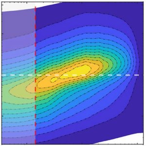
Contours of the power spectral density of the streamwise velocity fluctuation ( $k_x\phi _{uu}/{U_1^{2}}$) are plotted in figure 12 in terms of normalized wall distance (
 $y/\delta$) and wavelength (
 $\lambda _x/\delta$). We use Taylor's hypothesis of frozen turbulence (Taylor Reference Taylor1938) to obtain the wavenumber
  $k_x=2{{\rm \pi} }f/U_c$, where the convection velocity
  $U_c$ is approximated by the local mean velocity and
  $f$ is the frequency. It is generally accepted that this hypothesis is valid for both smooth- and rough-wall-bounded flows when the root mean square of fluctuating streamwise velocity
  $(u')$ is less than approximately 30 % of the local mean velocity (Lee, Lele & Moin Reference Lee, Lele and Moin1992; Romano Reference Romano1995; Squire et al. Reference Squire, Morrill-Winter, Hutchins, Schultz, Klewicki and Marusic2016). In the present study, the value of the ratio
  $u'/U$ is approximately 0.3 at a distance
  $y=k$ and decreases continuously as
  $y$ increases, as shown in figure 13 reporting the distribution of
  $u'/U$. Accordingly, we focus the spectral analysis on the region delimited
  $y=k$ (the vertical line in figure 12) where the Taylor hypothesis is appropriate (further discussions on the Taylor hypothesis for the present rough-wall TBL can be found in Ghanadi & Djenidi (Reference Ghanadi and Djenidi2021a)). Note that for clarity, the spectral analysis is carried out for location IV only; similar results are obtained for the other locations.

Figure 12. Premultiplied energy spectra of streamwise velocity fluctuation  $(k_x\phi _{uu}/{U_1}^{2})$ at location IV for the two different inlet velocities: (a–c)
  $U_{i,l}$; (d–f)
  $U_{i,h}$. Results are shown for FPG (a,d), ZPG (b,e) and APG (c,f). The red vertical line denotes the coordinate
  $y=k$ and the region
  $0 \leq y/k \leq 1$ is shaded. The dashed horizontal line indicates
  $\lambda _x=\delta$.

Figure 13. Profiles of  $u'/U_1$ as a function of
  $y/k$ at two streamwise locations, IV and V: (a–c)
  $U_{i,l}$; (d–f)
  $U_{i,h}$. See table 1 for symbols and colours.
In figure 12 one can observe the dynamic link between the large-scale structures in the outer region of the boundary layer and the regions closer to the roughness element. Comparing the velocity spectra between FPG (figure 12b) and APG (figure 12c) cases reveals a strong footprint of large-scale structures near the roughness element in rough-wall TBLs under APG; however, the interaction weakens with increasing  $Re$ (figure 12f). In the FPG case, the inner peak disappears or is fully submerged below the crest of the roughness elements (figure 12b,e). This indicates that flow accelerations in rough-wall TBLs under FPG assist the roughness elements to fully disrupt the viscous-dominated region near the wall. It can also be seen that the outer peak location in the FPG case occurs at a lower location compared with the APG case. This could be due to increasing the flow deceleration in the APG case leading to reducing the convection speed of the turbulent structures. We also notice first that, despite the the contours presenting similar shapes, there is, with respect to the line
  $\lambda _x/\delta =1$, a general ‘upward shift’ of the contours for the largest inlet velocity regardless of the PG; this is seen in the location (or locus) of the largest values of
  $(k_x\phi _{uu}/U_1^{2})$ (gold to yellow contours) in figure 12. This certainly reflects a Reynolds number effect. We also notice that this locus is at slightly lower values of
  $\lambda _x/\delta$ in the APG case than the ZPG and FPG cases. This latter feature suggests that APG affects the most energetic scales more than FPG when comparing with the ZPG case. In figure 14, the self-similar behaviour of the rough TBLs with PG through contour lines of velocity spectra can also be seen at the two last measurement locations. The results clearly demonstrate the self-similar behaviour of velocity spectra. Most importantly, the location of the outer peak as represented by the cross symbol in the figure does not change at these locations.

Figure 14. Comparison of contour lines of velocity spectra  $(k_x\phi _{uu}/{U_1}^{2})$ at locations IV and V for
  $U_{i,h}$: (a) FPG, (b) ZPG and (c) APG. The red vertical line denotes the coordinate
  $y=k$.
To ascertain possible differences between the effects of FPG and APG on the spectra we show in figure 15 the difference contours ( $k_x\phi ^{+}_{uu|\,PG}-k_x\phi ^{+}_{uu|\,ZPG}$) where the spectral contours for ZPG are subtracted from those for FPG and APG, respectively (the superscript
  $+$ represents normalization by
  $U_1$). In reference to the ZPG case, negative difference contours reveal a reduced energy level, while positive contours mark a higher energy level. Let us first focus on the lower inlet velocity,
  $U_{i,l}$ (figure 15a,b). There is no significant difference in the contours between FPG and APG in the region below
  $y/\delta \simeq 0.08$. In that region, the contours change sign from negative to positive; the ‘separation line’ between the negative and positive contours exhibits a positive slope (
 $\lambda _x/\delta$ increases with
  $y/\delta$) before it becomes practically horizontal. Notice the narrowing trend of the contours as the separation line is approached from below and above. The similarity of the difference contours between the PG cases suggests that the PG effect is not significant in that region and that the flow behaviour/dynamic is mostly controlled by the roughness. Above this roughness-controlled region (i.e.
  $y/\delta \geq 0.1$), one can observe a significant change between the FPG and APG cases. For the FPG case, the contours are now all negative, while there is still a change of sign for the APG case. This difference suggests that the TBL in this flow region is more receptive to PG than close to the wall. However, when the inlet velocity is increased to
  $U_{i,h}$ (figure 15c,d) one can observe marked differences between the two inlet velocity cases and the two PGs suggesting different dynamical behaviours of the TBL under the different PGs. For FPG, the negative contours initially observed in the region (
 $y/\delta \geq 0.1$) for
  $U_{i,l}$ are replaced by positive contours. For APG, the negative contours move up to larger values of
  $\lambda _x/\delta$ for
  $U_{i,h}$ (figure 15d) than for
  $U_{i,l}$ (figure 15b) in the region
  $y/\delta \leq 0.3$, while the positive contours almost vanish.

Figure 15. Contours of energy difference between APG/FPG and ZPG at location IV: (a,c)  $k_x\phi ^{+}_{uu|\,FPG}-k_x\phi ^{+}_{uu|\,ZPG}$ (dashed contours indicate negative values); (b,d)
  $k_x\phi ^{+}_{uu|\,APG}-k_x\phi ^{+}_{uu|\,ZPG}$. Results are shown for (a,b)
  $U_{i,l}$ and (c,d)
  $U_{i,h}$. The red and blue vertical lines denote the coordinates
  $y=k$ and
  $y=0.1 \delta$. Some contour values are shown for clarity.
Overall, figure 15 indicates that the differences between FPG and APG effects on the rough-wall TBL appear to be more pronounced with increasing Reynolds numbers, reflecting the results of figure 11. This is perhaps not too surprising considering the opposite effects that APG (deceleration) and FPG (acceleration) have on the flow. Clearly more studies at larger Reynolds numbers than here and over a longer streamwise distance (to achieve a clear sink flow in the case of FPG) are required to confirm or not this observation.
3.3. Proper orthogonal decomposition analysis
We turn our attention now to another approach for investigating the energy distribution between scales of motion in turbulent flows. This approach is based on the proper orthogonal decomposition (POD) method (Lumley Reference Lumley1967; Berkooz, Holmes & Lumley Reference Berkooz, Holmes and Lumley1993). In this method spatiotemporal streamwise velocity function  $u(x,t)$ is decomposed into spatial and temporal characteristics as
 \begin{equation} u(x,t)=\sum_{n}^{N_m} a_n(t) \psi_n(x), \end{equation}
where  $\psi _n(x)$ corresponds to the spatial orthonormal basis function (or eigenmodes),
  $a_n(t)$ are the time-dependent coefficients (often called random coefficients) and
  $N_m$ is the number of basis functions (or modes). A POD analysis, which is a generalization of power spectral analysis, decomposes the complex turbulent boundary layer flow into simpler modes, and thus complements the spectral analysis reported above. Indeed, while spectral analysis helps assess how the energy distribution among scales is affected by the PGs, the POD analysis, which contains information about the structure of the turbulent eddies (via the eigenvalues and eigenfunctions), helps determine how the individual features/events, particularly the most energetic ones, are affected. It is commonly agreed that the low-order modes are representative of large-scale motions and higher-order modes are associated with small-scale ones. Further, individual POD modes are also associated with particular events such as sweep and ejection events. A POD analysis is mostly carried out using velocity fields obtained using particle image velocimetry (Kruse, Kuhn & von Rohr Reference Kruse, Kuhn and von Rohr2006; Djenidi et al. Reference Djenidi, Antonia, Amielh and Anselmet2010; Druault, Bouhoubeiny & Germain Reference Druault, Bouhoubeiny and Germain2012; Shehzad et al. Reference Shehzad, Sun, Jovic, Ostovan, Cuvier, Foucaut, Willert, Atkinson and Soria2021). It has been shown, however, that POD can also be carried out using temporal velocity signals acquired via single hot-wire measurements (Tang et al. Reference Tang, Djenidi, Antonia and Zhou2014). This latter variant of POD is used in the present study. In such POD variant method the velocity signal is used to obtain a correlation matrix, written as
 \begin{equation} U = \begin{bmatrix} u(t_1) & u(t_2) & \cdots & u(t_n) \\ u(t_2) & u(t_3) & \cdots & u(t_n+1)\\ : & : & \cdots & : \\ u(t_{N_m}) & u(t_{{N_m}+1}) & \cdots. & u(t_{{N_m}+n-1}) \end{bmatrix}, \end{equation}
where  $n$ is the number of velocity samples,
  $N_m > > n$ and each column has approximately identical root-mean-square values with similar velocity spectra. The time separation between two consecutive velocity samples is selected such that the correlation
  $\overline {u(t)u(t+\tau )}$ drops to zero to ensure that the two velocities are uncorrelated (see Tang et al. (Reference Tang, Djenidi, Antonia and Zhou2014) for more details). Then the POD modes can be calculated as
 \begin{equation} \psi_n(x)=\frac{1}{\sqrt{\zeta_n}}U\upsilon_n, \end{equation}
where  $\zeta$ and
  $\upsilon$ are the eigenvalue and eigenvector of
  $U^{T}U$, respectively. Figure 16 shows the fractional contribution of the POD modes to the total kinetic energy,
  $\zeta _n/\sum _{n=1}^{N_t} \zeta _n$, at two wall-normal locations,
  $y/\delta = 0.1$ and 0.6 (for completeness we also report the cumulative energy contribution). Parameter
  $N_t$ is the total number of basis functions. The first mode contains the largest energy contribution, which varies between 40 % and 60 % for
  $U_{i,l}$ and approximately 25 %–50 % for
  $U_{i,h}$. That contribution drops to approximately 20 % for the second mode for both inlet velocities, while the third mode contributes approximately 10 % to the total energy. Interestingly, the contribution of the first mode is impacted by the PG. For example, that contribution is the largest for APG and the lowest for ZPG. Notably, the contribution of the second mode appears much less affected by the PG; it is practically the same for all three PGs. However, the third mode (and higher for that matter) does show a PG dependence, which is the reverse of that shown by the first mode. This behaviour difference between the modes under different PGs is yet to be physically explained. It nevertheless indicates not only the sensitivity of the large-scale motion to the PG, but also that the response of the TBL varies with the scales of motion as indicated by the non-trivial behaviour of the modes as described above. Indeed, in comparison with the ZPG case, an APG would strengthen the flow structures associated with the first mode as illustrated by the increase of their energy contribution and weaken the flow structures associated with third and higher modes, while leaving the structures represented by the second mode apparently unaffected. This non-trivial behaviour is perhaps best illustrated in figure 17 which shows the fractional contributions for the first three modes as a function of
  $y/\delta$. First, notice that the energy contribution of the second mode across the TBL is not much affected by the PGs. It is as if the flow structures associated with this mode are independent of PG. The situation for the first and third modes is different. For APG, the first- and third-mode contributions behave in opposite trends when compared with the other PGs across the TBL; the first mode is the largest and the third mode the smallest. These two modes have similar distributions of
  $\zeta$ across the TBL for the ZPG and FPG cases.

Figure 16. The POD fractional and cumulative energy contributions at location IV: (a,c)  $y/\delta = 0.1$; (b,d)
  $y/\delta = 0.6$. Open symbols are associated with
  $U_{i,l}$ and filled symbols are associated with
  $U_{i,h}$. Black, blue and red symbols represent ZPG, APG and FPG data, respectively. The black arrows indicate the axis corresponding to the cumulative energy plots.

Figure 17. The POD fractional contribution,  $\zeta _n/\sum _{n=1}^{N_t} \zeta _n$, as a function of
  $y/\delta$ at location IV for the first three modes for both inlet velocities: (a–c)
  $U_{i,l}$; (d–f)
  $U_{i,h}$. (a,d) First mode, (b,e) second mode and (c,f) third mode. Symbols are the same as in figure 16.
Figure 18 shows a log–log representation of the POD fractional energy reported in figure 16. This representation allows us to determine whether the decay of the fractional energy with an increasing mode order follows a power law of the form  $n^{\alpha }$. If such a power law exists, it should be reflected in a ‘linear’ decreasing trend in the data when reported in a log–log plot. Such a trend is clearly visible for the more or less first 15 modes when the inlet velocity is
  $U_{i,l}$, but not for
  $U_{i,h}$. Beyond these modes and while such a trend is less evident, one can nevertheless approximate the decay of the fractional energy by a power-law form with different exponents,
  $\alpha$, as represented by the lines tentatively drawn in figure 18; this is particularly more discernible for
  $U_{i,h}$ than for
  $U_{i,l}$. Notice that the magnitude of the decay exponent
  $\alpha$ is smaller for
  $U_{i,h}$ than for
  $U_{i,l}$. It is tempting to posit that the fractional energy decays in a ‘self-preserving’ manner with an increasing mode order. Note that the difference in the effects of the PGs on the decay is more visible at the lower inlet velocity than at the higher one. It is worthwhile commenting on the power-law trend. Indeed, it is difficult at this stage to link the power law (and its exponent
  $n$) to the physical nature of the TBL. One tentative interpretation would be that
  $n$ ‘measures’ the rate at which the energy is lost as the mode order increases. The higher the magnitude of
  $n$, the faster the decay of energy. This would suggest that a TBL with a large decay rate is predominantly composed of ‘energetic’ structures. Further analysis is required on this issue.

Figure 18. Log–log representation of the POD fractional energy at location IV: (a,c)  $y/\delta = 0.1$; (b,d)
  $y/\delta$= 0.6. Results are shown for (a,b)
  $U_{i,l}$ and (c,d)
  $U_{i,h}$. Black, blue and red symbols represent ZPG, APG and FPG data, respectively.
We close this POD analysis by showing in figure 19 examples of power spectral density,  $E_{a_n}(f)$, of the random coefficients
  $a_n(t)$ for modes 1, 2, 3, 5, 10 and 50 for all PGs at
  $y/\delta =0.1$ and both inlet velocities. One can observe that these power spectral densities exhibit a similar feature: a peak at a very low frequency. This peak indicates that the coefficients
  $a_n(t)$ draw their contents mostly from the frequency range 1–10 Hz. However, the peak magnitude decreases as
  $n$ increases; the peak has significantly reduced for
  $n=50$. This behaviour is consistent with the idea that the higher the mode order, the lower the contribution to the total energy, as illustrated in the fractional energy plot (see figure 16). There are some differences between the PGs. For example, the magnitude of the peak of mode 1 is larger for the ZPG case than for the APG and FPG cases. Notice also differences between the FPG and APG cases. Altogether the figure indicates that the features captured by the modes ‘oscillate’ at low frequencies and they respond to the PGs.

Figure 19. Power spectral density of the coefficients  $a_n(t)$ for modes 1, 2, 3, 5, 10 and 50 at location IV and
  $y/\delta$=0.1: (a–c)
  $U_{i,l}$; (d–f)
  $U_{i,h}$. Results are shown for (a,d) ZPG, (b,e) FPG and (c,f) APG.
4. Conclusion
Hot-wire measurements are carried out in a two-dimensional fully rough TBL under ZPG, FPG and APG with the view to help provide some elements of answers to the questions listed in the introduction. The following observations are made:
(i) The fully rough-wall TBL maintains its SP state as reflected by the linear growth of the boundary layer thickness. While this is not too surprising for ZPG and APG, it was unexpected for FPG. Indeed, under FPG, SP indicates
$\delta$ must decrease (sink flow). However, this is true when FPG is applied to a fully developed TBL. In the present case, the FPG is applied to a growing TBL.(ii) While a state of SP is observed, that state is likely to be dependent on PG, i.e. the TBL reaches different SP states under different PGs. This is suggested by the lack of collapse in the mean velocity between the different PG cases. A similar lack of collapse is also noted in the turbulence intensity profiles between the PG cases. Bobke et al. (Reference Bobke, Vinuesa, Örlü and Schlatter2017) also showed the same behaviour for a smooth wall by comparing TBLs subjected to PGs in near-equilibrium conditions at matched
$Re_\tau$.(iii) The premultiplied energy spectra between the different PGs are qualitatively similar in the region
$y/\delta \leq 0.1$, suggesting that the roughness effect is more important than the PG effects in this region. Beyond this region, though, the rough TBL appears to be sensitive to the PGs. For example, the energy spectra indicate that a significant amount of energy is reduced in the outer region of the boundary layer between the FPG and ZPG cases. Also, it is noted that for the APG case, increasing $Re$ weakens the effect of PGs on the boundary layer over the entire wavelength domain in the region $0.1 < y/\delta < 0.7$.


The above observations suggest that the rough-wall TBL under PGs responds first to the roughness and then to the PGs; the closer to the wall, the more dominant is the roughness effect. This is consistent with the finding of Ghanadi & Djenidi (Reference Ghanadi and Djenidi2021a), who showed that roughness prevents relaminarization downstream of a local wall suction (or equivalently strong local FPG). It is also worth noticing that the boundary layers in the present study are not fully developed and hence the values may change in scenarios where fully developed state is achieved.
Finally, a POD analysis was applied to the hot-wire signals. The analysis shows as expected that, across the boundary layer thickness, the first POD mode is the largest contributor to the total energy and regardless of  $Re$ is well impacted by the PGs. This is consistent with the results of the ‘classical’ energy spectra analysis reported above. Interesting, decay of the fractional (POD) energy can be approximated by a power-law form
  $n^{\alpha }$, where
  $n$ is the mode order and
  $\alpha$ is a negative number. Further study is required to confirm this and determine whether
  $\alpha$ is dependent on PG.
Funding
The authors gratefully acknowledge the support of the Australian Research Council, Discovery Project (ARC, DP190102751).
Declaration of interests
The authors report no conflict of interest.


