


1. Introduction
Wall-bounded turbulent flows over heterogeneous surfaces are prevalent in a wide range of practical situations. In industrial applications non-uniform flows occur in internal flow systems such as flow through pipes and ducts, marine transportation or turbomachinery (Medjnoun et al. Reference Medjnoun, Rodriguez-Lopez, Ferreira, Griffiths, Meyers and Ganapathisubramani2021). A well-known example in the environment is the atmospheric boundary layer (ABL), where one can think of land-sea breezes, urban-rural transitions, wind-farm boundary layers, airflow over lakes and land-surface exchange over patchy agricultural terrain for instance (Bou-Zeid et al. Reference Bou-Zeid, Anderson, Katul and Mahrt2020). Moreover, such flows are often stably stratified (Stull Reference Stull1988; Zonta & Soldati Reference Zonta and Soldati2018). Flow heterogeneity and stratification can considerably affect momentum transfer in the fluid and heat transfer between the surface and the fluid, and is therefore of special interest for the engineering and atmospheric community. In the present work we use direct numerical simulations (DNS) to study stably stratified channel flow with spanwise heterogeneous surface temperature. We examine the influence of the spanwise length scale of the heterogeneity ( $\lambda /h$), the Reynolds number, the stability of the flow and the upper boundary conditions. We focus on the effect of the thermal heterogeneity on the mean flow structures and the momentum and heat transfer.
Neutral flows over non-uniform surfaces have been studied extensively in the past years in field studies, wind-tunnel experiments as well as numerical simulations. A widely used example is the flow over a rough surface, which can be further divided into homogeneous and heterogeneous roughness (Medjnoun, Vanderwel & Ganapathisubramani Reference Medjnoun, Vanderwel and Ganapathisubramani2018). The presence of surface roughness alters the well-known logarithmic mean velocity profile that applies to smooth walls. There currently exist well-established empirical scaling laws and methods for predicting turbulent flows over a spatially uniform rough surface such as the modified logarithmic profile (Nikuradse Reference Nikuradse1933), and for pipe flow there is the Moody chart (Chung, Monty & Hutchins Reference Chung, Monty and Hutchins2018). Both methods are based on a vertical roughness length scale, and on the classical picture that the roughness-induced motions are confined to the roughness sublayer, close to the wall.
By contrast, in recent years, it was found that roughness arrangements with dominant spanwise length scales of the order of the boundary layer height excite large secondary motions that penetrate into the outer layer of the flow (Barros & Christensen Reference Barros and Christensen2014; Anderson et al. Reference Anderson, Barros, Christensen and Awasthi2015; Vanderwel & Ganapathisubramani Reference Vanderwel and Ganapathisubramani2015; Kevin et al. Reference Kevin, Monty, Bai, Pathikonda, Nugroho, Barros, Christensen and Hutchins2017; Hwang & Lee Reference Hwang and Lee2018; Medjnoun et al. Reference Medjnoun, Vanderwel and Ganapathisubramani2018). These motions significantly affect the mean flow profile, such that simple parametrizations based on roughness length do not suffice. The present work explores spanwise heterogeneities with these specific length scales, but employs surfaces with heterogeneous temperature instead of heterogeneous roughness arrangements.
1.1. Secondary flows
The phenomenon of secondary flows was already considered many years ago, for example, in the duct flow community (Bradshaw Reference Bradshaw1987) and, more recently, in the hydraulic engineering community (e.g. Wang & Cheng Reference Wang and Cheng2005; Vermaas, Uijttewaal & Hoitink Reference Vermaas, Uijttewaal and Hoitink2011). For a historical overview of scientific literature concerning secondary flows, one can read, for example, the introduction of Medjnoun, Vanderwel & Ganapathisubramani (Reference Medjnoun, Vanderwel and Ganapathisubramani2020). Lately, secondary flows have been observed in both experimental (Barros & Christensen Reference Barros and Christensen2014; Anderson et al. Reference Anderson, Barros, Christensen and Awasthi2015; Kevin et al. Reference Kevin, Monty, Bai, Pathikonda, Nugroho, Barros, Christensen and Hutchins2017; Medjnoun et al. Reference Medjnoun, Vanderwel and Ganapathisubramani2018, Reference Medjnoun, Vanderwel and Ganapathisubramani2020) and numerical studies of flow over spanwise heterogeneous roughness arrangements. In the numerical studies two kinds of boundary conditions that generate the secondary flows can be distinguished. The inhomogeneity is either created by a variation in surface elevation (Hwang & Lee Reference Hwang and Lee2018; Yang & Anderson Reference Yang and Anderson2018; Stroh et al. Reference Stroh, Schäfer, Forooghi and Frohnapfel2020), comparable to a real-world topography, or by directly prescribing a varying wall shear stress (Anderson et al. Reference Anderson, Barros, Christensen and Awasthi2015; Vanderwel & Ganapathisubramani Reference Vanderwel and Ganapathisubramani2015; Vanderwel et al. Reference Vanderwel, Stroh, Kriegseis, Frohnapfel and Ganapathisubramani2019; Forooghi, Yang & Abkar Reference Forooghi, Yang and Abkar2020). Regarding the generation mechanism of the mean secondary motions over spanwise heterogeneous roughness, Anderson et al. (Reference Anderson, Barros, Christensen and Awasthi2015) demonstrated that they are a realization of Prandtl's secondary flow of the second kind, driven and sustained by spatial heterogeneity of the spanwise-wall-normal Reynolds stress components (Yang & Anderson Reference Yang and Anderson2018). The secondary flows are characterized by the formation of vortices in the plane normal to the flow direction, where the related upward and downward motions introduce low-momentum pathways (LMPs) and high-momentum pathways (HMPs) in the mean streamwise velocity distribution. The location of the LMPs and HMPs and the rotational direction of the secondary motions are still an object of ongoing discussion (Stroh et al. Reference Stroh, Schäfer, Forooghi and Frohnapfel2020). Besides, flow heterogeneity intrinsically introduces dispersive fluxes (Raupach & Shaw Reference Raupach and Shaw1982), which arise due to local deviations from the horizontal mean velocity or temperature (see § 2.3).
Several studies have investigated the dependency of the size and strength of the secondary vortices on the spanwise heterogeneity length scale, e.g. Chung et al. (Reference Chung, Monty and Hutchins2018) and Medjnoun et al. (Reference Medjnoun, Vanderwel and Ganapathisubramani2018). The latter divide spanwise heterogeneous flows into three different regimes based on the spanwise heterogeneity scale. In regime A the spanwise length scale of the heterogeneity is much smaller than the height of the boundary layer ( $\lambda /h \ll 1$), and the secondary flows are so small that they are confined to the roughness sublayer such that the outer flow still remains ‘homogeneous.’ In regime B,
  $\lambda /h \approx 1$, and secondary flows occupy a large portion of the flow such that their effect extends through the entire boundary layer. As a result, the flow is highly three dimensional and local similarity does not hold. Finally, in regime C, where
  $\lambda /h \gg 1$, there will still be heterogeneous regions close to the surface discontinuity but the flow would be homogeneous far away from them. In the present work we aim to examine these regimes for spanwise heterogeneous surface temperature rather than roughness.
The effect of surface roughness and secondary flows on heat and momentum transfer has not been explored extensively yet, although some recent numerical studies have incorporated temperature as a passive scalar, thus neglecting stratification effects. Leonardi et al. (Reference Leonardi, Orlandi, Djenidi and Antonia2015) studied passive heat transfer in a turbulent channel flow with square bars and circular rods on the bottom wall, and found that heat transport is enhanced due to induced ejection at the leading edge of the roughness elements, while the skin friction was increased as well. Moreover, they found that the Reynolds analogy, which states that momentum and heat transfer are proportional, is not valid close to the wall. We note however that the roughness elements here were oriented in the spanwise direction, as opposed to spanwise heterogeneous roughness that was discussed before. Stroh et al. (Reference Stroh, Schäfer, Forooghi and Frohnapfel2020) analysed the effect of secondary flows caused by streamwise ridges on passive heat transfer. They state that momentum and heat transfer are enhanced by approximately 30 % relative to a smooth channel, whereas the ratio of Stanton number (describing heat transfer) to friction coefficient is close to the smooth channel value.
1.2. Stably stratified channel flow
The two studies mentioned above only considered the effect of the flow on the temperature distribution, and not vice versa. By contrast, the present work does include stratification effects through the buoyancy force. We focus on stable stratification, because of its relevance in environmental engineering and geophysical applications. Stably stratified boundary layers generally occur when warm fluid is advected over a colder surface (Mahrt Reference Mahrt2014), such as warm air over cold seas or ice as in polar regions. Oceanic flows are almost always stably stratified (Wunsch & Ferrari Reference Wunsch and Ferrari2004), while the ABL over land is typically stably stratified at night, or in summertime over sea (Stull Reference Stull1988; Wyngaard Reference Wyngaard2010). Stably stratified wall-bounded turbulence is moreover common in industrial processes such as cooling in nuclear reactors, fluid motion in heat transfer equipment and fuel injection and combustion in gasoline engines (Zonta & Soldati Reference Zonta and Soldati2018).
Stably stratified turbulence is regarded as a truly complicated problem in fluid dynamics, even in absence of horizontal heterogeneity. Despite much research into (horizontally homogeneous) turbulent flows with stable stratification, our understanding remains incomplete and models are often insufficient to fully describe their behaviour, especially in the very stable regime (Mahrt Reference Mahrt2014). In wall-bounded flows turbulent kinetic energy (TKE) is produced by the shear due to the presence of the wall, whereas the negative buoyancy force acts as a destructive force on the vertical motions and has a negative effect on the TKE budget. The dynamics in stably stratified turbulence are thus governed by these two competing mechanisms, which are fundamentally different in nature (see, e.g. Wyngaard Reference Wyngaard2010, p. 268).
Numerical studies that investigated stably stratified flows have reported that with increasing stratification, the turbulence is dampened so much that it becomes intermittent in time and laminar-turbulent patches coexist near the wall, until a critical stratification level is reached where all turbulence is extinguished and the flow becomes laminar (e.g. Nieuwstadt Reference Nieuwstadt2005; Flores & Riley Reference Flores and Riley2011; García-Villalba & del Álamo Reference García-Villalba and del Álamo2011; He & Basu Reference He and Basu2015; van Hooijdonk et al. Reference van Hooijdonk, Clercx, Ansorge, Moene and van de Wiel2018; Atoufi, Scott & Waite Reference Atoufi, Scott and Waite2019). Long before, Gage & Reid (Reference Gage and Reid1968) had already developed a linear stability theory for homogeneous stratified plane Poiseuille flow, and found an explicit relation between the Reynolds number of the flow and the critical Richardson number at which the flow becomes stable. Although first attempts of numerical simulations with stably stratified plane channel flow showed turbulence collapse already at much lower Richardson numbers then those predicted by linear theory (Garg et al. Reference Garg, Ferziger, Monismith and Koseff2000; Iida, Kasagi & Nagano Reference Iida, Kasagi and Nagano2002), more recent DNS and LES results were consistent with this theory. It was demonstrated that a large enough domain size is crucial to maintain the turbulence (Flores & Riley Reference Flores and Riley2011; García-Villalba & del Álamo Reference García-Villalba and del Álamo2011), while other authors suggest that the laminarization is also sensitive to the choice of boundary and initial conditions and the type of forcing to the flow (Brethouwer, Duguet & Schlatter Reference Brethouwer, Duguet and Schlatter2012; van Hooijdonk et al. Reference van Hooijdonk, Clercx, Ansorge, Moene and van de Wiel2018). Numerical studies in the ABL community have focused on finding a stability threshold for turbulence collapse expressed in a different parameter than the Richardson number, such as a critical Obukhov length (Nieuwstadt Reference Nieuwstadt2005), Obukhov-Reynolds number (Flores & Riley Reference Flores and Riley2011; Deusebio et al. Reference Deusebio, Brethouwer, Schlatter and Lindborg2014; Zhou, Taylor & Caulfield Reference Zhou, Taylor and Caulfield2017) or ‘shear capacity’ (Donda et al. Reference Donda, van Hooijdonk, Moene, van Heijst, Clercx and van de Wiel2016; van Hooijdonk et al. Reference van Hooijdonk, Clercx, Ansorge, Moene and van de Wiel2018). Moreover, Donda et al. (Reference Donda, van Hooijdonk, Moene, Jonker, van Heijst, Clercx and van de Wiel2015) argue that turbulence collapse is only temporary, and turbulence is regenerated due to increased shear in the laminar state in combination with small perturbations. Despite the differences in the choice of velocity and temperature boundary conditions in all these numerical studies, the collapse of turbulence due to a stable density or temperature gradient appears to be controlled by the same mechanisms in different wall-bounded flow configurations (Zhou et al. Reference Zhou, Taylor and Caulfield2017; van Hooijdonk et al. Reference van Hooijdonk, Clercx, Ansorge, Moene and van de Wiel2018).
In the context of the present paper, it is relevant to note that the aforementioned numerical studies of stratified turbulence only considered horizontally homogeneous flows, and that heterogeneous stratified turbulence is covered less often. Nevertheless, Flores & Riley (Reference Flores and Riley2011) compare their results to a measurement campaign over flat open prairy grass in Kansas (CASES-99, Poulos et al. Reference Poulos2002), and suggest that their criterion for turbulence collapse over smooth surfaces, based on a Reynolds number with the Obukhov length ( $Re_L < 10^2$), can be extended to rough surfaces. Druzhinin, Troitskaya & Zilitinkevich (Reference Druzhinin, Troitskaya and Zilitinkevich2016) performed DNS of a turbulent Couette flow over a (streamwise) waved water surface and confirm that indeed this ‘
 $Re_L$-condition’ holds for flow over waved surfaces as well, but if the wave slope is sufficiently steep the velocity and temperature fluctuations are maintained even for supercritical stratification. Williams et al. (Reference Williams, Hohman, Van Buren, Bou-Zeid and Smits2017) performed wind-tunnel experiments to study the effect of stable stratification on turbulent boundary layers over smooth and rough walls, and report that the bulk Richardson number at which turbulence collapses is 1.5 times larger for the rough wall compared with the smooth wall. Moreover, they note that their wind-tunnel results are consistent with the
  $Re_L$-condition obtained by the DNS from Flores & Riley (Reference Flores and Riley2011), and even correspond with atmospheric observation data from Sorbjan (Reference Sorbjan2010), suggesting that many aspects of the atmospheric surface layer can be investigated from stably stratified (laboratory) experiments at relatively low Reynolds number.
Besides the phenomenon of turbulence collapse, strong stratification significantly reduces wall-normal heat and momentum transfer rates in a turbulent channel compared with neutral cases (Zonta & Soldati Reference Zonta and Soldati2018). Traditional ways to quantify heat and momentum transfer in stable channel flow are the Nusselt number and friction coefficient, respectively (Armenio & Sarkar Reference Armenio and Sarkar2002; Iida et al. Reference Iida, Kasagi and Nagano2002; García-Villalba & del Álamo Reference García-Villalba and del Álamo2011). Qualitatively, it is known that stable stratification reduces the average transport of momentum and heat compared with the neutrally buoyant case (Armenio & Sarkar Reference Armenio and Sarkar2002). From an engineering point of view, empirical correlations exist to calculate the Nusselt number in many different configurations, mostly based on either forced or natural convection regimes. However, most forced convection correlations neglect buoyancy effects (Mills & Coimbra Reference Mills and Coimbra1999, p. 308). Hence, such simple correlations do not exist for mixed convection in stably stratified boundary layers (Zonta Reference Zonta2013), let alone heterogeneous flows.
Despite the lack of well-established parametrizations for heat and momentum transfer in stable channel flows, García-Villalba & del Álamo (Reference García-Villalba and del Álamo2011) made an attempt based on their stable channel flow DNS database, and report that the friction coefficient seems to scale with the shear Richardson number as  $C_f \propto Ri_\tau ^{-1/3}$, independent of the Reynolds number. By combining results of various numerical and experimental studies that involved stable channel flow, Zonta & Soldati (Reference Zonta and Soldati2018) show that this relation seems to hold fairly well even for larger Reynolds and Richardson numbers, although a proper theoretical understanding for this law is missing. They furthermore report that the Nusselt number data does not collapse to a correlation of
  $Ri_\tau$ only, as it also increases with increasing Reynolds number. The present work aims to explore these kind of correlations in the context of stably stratified inhomogeneous flows.
1.3. Stratified heterogeneous flows
The concepts of secondary flows and stable stratification were for the first time combined in the recent work by Forooghi et al. (Reference Forooghi, Yang and Abkar2020), through conducting LES of open channel flow with spanwise-adjacent strips of high and low surface roughness at different stratification levels. Their results indicate that the size and strength of the secondary vortices are reduced by the stable stratification, which is known to suppress vertical motions. Interestingly, the shear near the top of the wall-adjacent vortex generates a second vortex on top of the first, eventually leading to a stack of secondary vortices with decreasing strength away from the wall. The authors note that this was only a first attempt to shed light on the effect of thermal stratification on roughness-induced secondary flows, and further investigations, including DNS at low Reynolds number as in the present study, are needed to get a better picture of the problem.
In all the above-mentioned work, surface heterogeneity was introduced by varying topology height or the shear stress boundary condition. In the ABL however, temperature (or heat flux) variations over the surface are also abundant. Accurate parametrization of non-uniform surface temperature is crucial for numerical models that are used for weather and climate prediction. Some studies in the past decade investigated flow over surfaces with heterogeneous thermal boundary conditions, most of which used LES and considered either streamwise heterogeneous temperature patches (Stoll & Porté-Agel Reference Stoll and Porté-Agel2009; Mironov & Sullivan Reference Mironov and Sullivan2016) or two-dimensional patches (Roo & Mauder Reference Roo and Mauder2018; Margairaz, Pardyjak & Calaf Reference Margairaz, Pardyjak and Calaf2020).
Stoll & Porté-Agel (Reference Stoll and Porté-Agel2009) investigated a stable boundary layer (SBL) flow over a surface with high- and low-temperature patches in the streamwise direction, where temperature differences of 3 and 6 K were used. They report significant effects on mean wind speed and temperature profiles, with higher turbulence levels and more vertical mixing compared with a homogeneous case. Moreover, they conclude that standard Monin–Obukhov similarity theory, that is commonly used to relate the average surface heat flux and potential temperature at the first level of a large-scale model, leads to significant errors for heterogeneous flows. Mironov & Sullivan (Reference Mironov and Sullivan2016) used a similar configuration but with a sinusoidal variation of the surface temperature instead of discrete patches, and conclude that the temperature variance and its budget play a crucial role in a heterogeneous SBL. Moreover, both studies report that the magnitude of the temperature difference between the warm and cold stripes has a pronounced effect on the SBL structure, while the results were practically independent on the streamwise length scale of the heterogeneity which was varied between 100 and 400 m. The authors hypothesize that this might change in the strongly stable regime, and suggest that future work should investigate this issue. The present work does indeed investigate strongly stable flows, but uses temperature variation in the spanwise direction instead of the streamwise direction.
Surface temperature variations have also been numerically investigated in a (free) convective boundary layer (CBL), where the flow is heated from below, with streamwise patches (Patton, Sullivan & Moeng Reference Patton, Sullivan and Moeng2005) and later two-dimensional chessboard patterns (Brunsell, Mechem & Anderson Reference Brunsell, Mechem and Anderson2011; Van Heerwaarden, Mellado & de Lozar Reference Van Heerwaarden, Mellado and de Lozar2014; Roo & Mauder Reference Roo and Mauder2018; Margairaz et al. Reference Margairaz, Pardyjak and Calaf2020). Common findings indicate that surface heterogeneity with length scales of the same order of magnitude as the boundary layer depth and larger (i.e. kilometre scale for a typical CBL in the atmosphere) have the largest effect on the full boundary layer structure, while heterogeneity at smaller scales is blended in the surface layer (Roo & Mauder Reference Roo and Mauder2018). This seems to be consistent with the picture of the secondary motions generated by spanwise heterogeneous roughness with similar length scales, as described in § 1.1. Based on their LES results, Roo & Mauder (Reference Roo and Mauder2018) moreover hypothesize that these landscape-scale surface heterogeneities could be the cause of an imbalance in the measured Earth surface heat flux, which is an unresolved problem in boundary layer meteorology. Margairaz et al. (Reference Margairaz, Pardyjak and Calaf2020) stress the importance of dispersive fluxes based on LES of flow over patches with randomly distributed temperatures, and propose the use of these dispersive fluxes as a measure of the footprint that surface thermal heterogeneities have on the flow. These dispersive fluxes are extensively examined in this work.
1.4. Scope of this study
The present study combines the elements described above, namely spanwise heterogeneity, stably stratified flow and thermally heterogeneous boundary conditions. That is, we explore the effect of spanwise heterogeneous surface temperature in (moderately to strongly) stably stratified channel flow. In general, we address the effect of the thermal heterogeneities on the statistical quantities of the velocity and thermal fields. We aim to get insight in how momentum and heat transfer in stratified channels is affected by temperature heterogeneities with varying length scales, and whether there are similarities with spanwise heterogeneous roughness arrangements. In addition, we compare results of homogeneous and heterogeneous channels under moderate and strong stratification to see how phenomena like turbulence intermittency and collapse are influenced, related to the key question whether turbulence survives longer over a heterogeneous surface (Mironov & Sullivan Reference Mironov and Sullivan2016).
The configuration that we consider consists of strips of high and low temperature with equal width at the bottom and top boundaries of a pressure-driven channel flow. In addition to the horizontal temperature variation, an average vertical temperature difference across the channel is maintained to induce an overall stable stratification. We assess the sensitivity of the flow to several key parameters. The lateral length scale of the temperature pattern is varied and two different arrangements of the upper boundary condition are considered: an ‘in-phase’ arrangement where the high- and low-temperature patches are vertically aligned and an ‘antiphase’ arrangement where the temperature pattern at the top wall is shifted by half of the wavelength (roughly similar to the symmetric and staggered arrangements of Stroh et al. Reference Stroh, Schäfer, Forooghi and Frohnapfel2020). Besides, we perform simulations with two different Reynolds and Richardson numbers to assess their influence on the flow.
While many of the above-mentioned studies used LES, we opt for DNS to avoid the need of any parametrization. On the one hand, the closure paradigms on which subgrid-scale models in LES are based are violated in strongly stratified, intermittent turbulence (Mironov & Sullivan Reference Mironov and Sullivan2016; van Hooijdonk et al. Reference van Hooijdonk, Clercx, Ansorge, Moene and van de Wiel2018). On the other hand, surface boundary conditions in LES rely on the Monin–Obukhov similarity theory, which in itself is based on homogeneous flow conditions and is therefore not valid in our configuration. The most obvious drawback of DNS is the very high computational cost, which significantly limits the Reynolds number that can be studied. Although the two different Reynolds numbers that we consider are much lower then geophysical values, DNS is generally regarded as an attractive tool to obtain at least qualitative insight, which should however be complemented with different SBL-modelling approaches that are able to represent higher-Reynolds-number flows like LES (Donda et al. Reference Donda, van Hooijdonk, Moene, Jonker, van Heijst, Clercx and van de Wiel2015).
It is worth noting that besides the relatively low Reynolds numbers, many other simplifications separate our set-up from real-world flows, as is usually done in DNS studies. For example, we do not account for any surface roughness effects, and the Coriolis force that causes a height-dependent wind direction in the ABL is ignored. This allows us to focus solely on the temperature effects, but these limitations must be taken into account when comparing our results with the real-world ABL or industrial situations. Another obvious dissimilarity between our full-channel geometry and the ABL is the no-slip boundary condition at the top. However, this geometry has been widely used in previous studies (e.g. Armenio & Sarkar Reference Armenio and Sarkar2002; García-Villalba & del Álamo Reference García-Villalba and del Álamo2011; van Hooijdonk et al. Reference van Hooijdonk, Clercx, Ansorge, Moene and van de Wiel2018), which have shown that it exhibits features generic to stably stratified wall-bounded flows. Therefore, our results can be considered relevant to a wide range of stably stratified boundary layers, e.g. the surface layer of the ABL.
Finally, the paper is further organized as follows. Section 2 describes the details of the simulations and the numerical code that was used. Results are presented and discussed in § 3, starting with a general description of velocity and temperature fields (§ 3.1), followed by a discussion on global momentum and heat transfer coefficients (3.2). In § 3.3 we focus on the high-Reynolds-number simulations and present a triple decomposition of the velocity and temperature field. The effect of increased stability and shifted upper wall temperature are addressed in §§ 3.4 and 3.5. The main conclusions are summarized in § 4.
2. Numerical methodology
2.1. Governing equations and DNS code
In this study DNS is used to study pressure-driven turbulent closed channel flow under stable stratification, where either homogeneous or spanwise heterogeneous wall temperatures are imposed. The Einstein summation convention is used in this section and the three spatial coordinates are denoted with  $(x_1, x_2, x_3) = (x, y, z)$, respectively the streamwise, spanwise and wall-normal (vertical) directions. Likewise, the velocity vector is
  $(u_1, u_2, u_3) = (u, v , w)$. Under the Boussinesq approximation and assuming incompressibility, the continuity, momentum and potential temperature equations correspond to
 $$\begin{gather} \frac{\partial u_i}{\partial x_i} = 0, \end{gather}$$
 $$\begin{gather}\frac{\partial u_i}{\partial t} +\frac{\partial u_i u_j}{\partial x_j} ={-}\frac{\partial p}{\partial x_i} + F_p\delta_{i1} + \frac{1}{{Re}_\tau} \frac{\partial^2u_i}{\partial x_j \partial x_j} + Ri^z_\tau \theta'' \delta_{i3}, \end{gather}$$
 $$\begin{gather}\frac{\partial \theta}{\partial t} + \frac{\partial u_j \theta}{\partial x_j} = \frac{1}{{Re}_\tau {Pr}}\frac{\partial^2\theta}{\partial x_j \partial x_j}. \end{gather}$$
The governing equations are normalized by the half-channel height  $h( = 1)$ and the friction velocity
  $u_\tau = ( \tau _w /\rho _0 )^{1/2}$ (e.g.
  $u_i = u_i^* / u_\tau$,
  $x_i = x^*/h$, with the ‘
 $^*$’ denoting the dimensional value), where
  $\tau _w$ is the wall shear stress and
  $\rho _0$ is a reference density. The flow is driven by a fixed mean pressure gradient
  $F_p$, which also fixes the friction velocity
  $u_\tau$. Further,
  $\delta _{ij}$ is the Kronecker-delta operator, which ensures that the flow is driven in the
  $x$-direction. The variable
  $p$ in (2.2) is the (non-dimensional) pressure fluctuation around the background pressure, i.e.
  $p_{\textit {tot}} = p - F_p(x-x_0)$. Further,
  ${Re}_\tau = u_\tau h/\nu$ is the friction Reynolds number. In the transport equation for the scalar potential temperature (2.3), we set the Prandtl number to 0.71 in order to represent air flow.
The last term in (2.2) represents the buoyancy force, where  $\theta ''=\theta - \langle \theta \rangle$ is the temperature deviation from the horizontal mean. Throughout this paper, we use
  $\langle \cdot \rangle = \langle \cdot \rangle _{xy}$ to indicate horizontally averaged variables. Using
  $\theta ''$ rather than
  $\theta$ is straightforward in a pseudo-spectral code, because the horizontally averaged buoyancy force can easily be set to 0. We remark that using
  $\theta ''$ or
  $\theta$ does not make a difference in the final results, since the difference is a (non-dimensional) potential force, which can be simply absorbed into the vertical pressure distribution. A similar approach was used by, for example, Garg et al. (Reference Garg, Ferziger, Monismith and Koseff2000), Armenio & Sarkar (Reference Armenio and Sarkar2002) and Stoll & Porté-Agel (Reference Stoll and Porté-Agel2008).
Further, the stability is determined by the friction Richardson number, commonly defined as  $Ri^z_\tau = \langle \Delta ^z\theta ^* \rangle g h / (\theta _0 u_\tau ^2)$, with
  $\theta _0$ the reference temperature and
  $\langle \Delta ^z\theta ^* \rangle = \langle \theta ^*_{t} \rangle - \langle \theta ^*_{b}\rangle$ the spatially averaged temperature difference between the top and bottom. The superscript
  $z$ is used here to emphasize that this Richardson number is based on the mean vertical temperature difference, as opposed to the horizontal temperature difference at the boundaries (see below). In the remainder of this paper we mean
  $Ri_\tau ^z$ by the Richardson number
  $Ri_\tau$, unless explicitly stated otherwise by a different superscript. We note that most ABL studies typically consider the potential temperature to parametrize buoyancy, while more fundamental stable channel flow studies consider the fluid density and base their
  $Ri_\tau$ on the vertical density difference (Garg et al. Reference Garg, Ferziger, Monismith and Koseff2000; Armenio & Sarkar Reference Armenio and Sarkar2002; García-Villalba & del Álamo Reference García-Villalba and del Álamo2011). However, the Boussinesq approximation provides a linear relation between temperature and density fluctuations and allows us to use either one of them as an independent variable (Wyngaard Reference Wyngaard2010; Allaerts Reference Allaerts2016), such that both definitions of
  $Ri_\tau$ are equivalent. The potential temperature is normalized with the vertical temperature difference across the channel,
  $\theta = (\theta ^*-\langle \theta ^*_{b}\rangle )/$
 $\langle \Delta ^z\theta ^* \rangle$, such that
  $\langle \theta _{b} \rangle = 0$ at the bottom and
  $\langle \theta _{t} \rangle = 1$ at the top.
Previous numerical studies that considered stably stratified wall-bounded turbulence used a variety of boundary conditions. For example, Nieuwstadt (Reference Nieuwstadt2005), Flores & Riley (Reference Flores and Riley2011), Brethouwer et al. (Reference Brethouwer, Duguet and Schlatter2012), Deusebio et al. (Reference Deusebio, Brethouwer, Schlatter and Lindborg2014), He & Basu (Reference He and Basu2015), He (Reference He2016) and Atoufi, Scott & Waite (Reference Atoufi, Scott and Waite2020) simulated open channel flow with a no-slip condition at the bottom and either a symmetry condition or fixed velocity at the top. Closed channel flow can be simulated with no-slip conditions on both the bottom and top walls (Garg et al. Reference Garg, Ferziger, Monismith and Koseff2000; Armenio & Sarkar Reference Armenio and Sarkar2002; García-Villalba & del Álamo Reference García-Villalba and del Álamo2011; He Reference He2016), while the plane Couette flow, where the upper and lower walls move with a fixed opposite velocity, has also been used to numerically investigate stably stratified boundary layers (García-Villalba, Azagra & Uhlmann Reference García-Villalba, Azagra and Uhlmann2011; Zhou et al. Reference Zhou, Taylor and Caulfield2017; van Hooijdonk et al. Reference van Hooijdonk, Clercx, Ansorge, Moene and van de Wiel2018). For the temperature, combinations of Dirichlet or Neumann conditions can be used to fix the respective temperature or heat flux at the upper and lower domain walls. In the present work we study closed channel flow and employ fixed temperature boundary conditions because of its relative simplicity and because a statistically steady state is reached with this set-up. Moreover, there is no clear hierarchy between imposing a constant heat flux or isothermal walls in terms of how realistically an ABL flow is represented (van Hooijdonk et al. Reference van Hooijdonk, Clercx, Ansorge, Moene and van de Wiel2018). Therefore, all velocity components are set to 0 at the upper and lower domain boundaries ( $z = 0$ and
  $2h$), and the temperatures at the upper and lower boundaries are fixed.
The LES/DNS code SP-wind, developed at KU Leuven, is used to solve the governing equations (2.1)–(2.3) with the aforementioned boundary conditions. In the horizontal directions a pseudo-spectral Fourier–Galerkin discretization with periodic boundary conditions is employed, while a fourth-order staggered finite-difference scheme (Verstappen & Veldman Reference Verstappen and Veldman2003) is used in the vertical direction. Nonlinear terms are computed in real space with the 3/2-dealiasing rule. Time integration is based on a classic fourth-order Runge–Kutta scheme, and the timestep is constrained by the minimum of the convective and viscous Courant–Friedrichs–Lewy (CFL) conditions, where the CFL number is set to 0.4. The continuity equation is imposed by solving a Poisson equation for the pressure.
The code has been widely used for LES of (stratified) boundary layers, also including wind turbines, but less often for DNS of stably stratified channel flow (Allaerts Reference Allaerts2016). In order to enable heterogeneous temperature boundary conditions, the temperature implementation in the code was slightly adapted by the present author. Therefore, a number of simulations of homogeneous stable channel flow was performed to verify our code against previous DNS studies (cf. Appendix A for results and discussion).
2.2. Simulation set-up
An overview of all simulations that are discussed in this paper is provided in table 1. To save on computational cost, the majority of simulations that were performed have a relatively low friction Reynolds number of  $Re_\tau = 180$. In most cases, the stratification is moderately stable with
  $Ri_\tau = 120$. To assess the dependence of our results to the Reynolds and Richardson number, we performed two additional sets of simulations: one where we increased
  $Re_\tau$ to 550 (indicated with Re550 in tables 1 and 2) and a set with strong stratification,
  $Ri_\tau = 960$ (indicated with Ri960 in table 1).
Table 1. Overview of simulations and some integral flow properties. Here  $Re_b = u_b h/\nu$ is the bulk Reynolds number, while
  $Ri_b = \langle \Delta ^z\theta \rangle g h / (2\theta _0 u_b^2)$ is the bulk Richardson number. Further,
  $h/L_{MO}$ is the stability parameter (Nieuwstadt Reference Nieuwstadt2005), where
  $L_{MO} = u_\tau ^3/(\kappa ( g/\theta _0) \alpha (\partial \langle \bar {\theta }\rangle /\partial z)_w )$ is the Obukhov length. These bulk properties are reported for completeness and easy comparison to studies with a different set-up, all other quantities are described and discussed in the text.

Table 2. Domain size and resolution for the cases with  $Re_\tau = 180$ and
  $Re_\tau =550$. Here
  $N_x$ and
  $N_y$ are the number of Fourier coefficients in the streamwise and spanwise directions, while
  $N_z$ is the number of grid points in the wall-normal direction. Grid resolutions are scaled with
  $\nu /u_\tau$ (e.g.
  $\Delta x^+ = \Delta x u_\tau /\nu$). The smaller and larger values of
  $\Delta z^+$ represent the vertical grid size at the walls and in the channel centre, respectively.

The dimensions of the domain for the Re180 simulations are  $L_x \times L_y \times L_z = 8{\rm \pi} h \times 4{\rm \pi} h \times 2h$, with grid resolution
  $N_x \times N_y \times N_z = 512 \times 512 \times 128$. The grid in the wall-normal direction is stretched using a hyperbolic tangent function, such that
  $\Delta z^+ = \Delta z u_\tau / \nu$ ranges from 0.3 at the wall to 6.3 in the channel centre. The simulation domain properties are summarized in table 2. We point out that this resolution is very close to previous stable channel flow DNS studies of García-Villalba & del Álamo (Reference García-Villalba and del Álamo2011) and He & Basu (Reference He and Basu2016). Moreover, we validated our SP-wind code with this domain size and resolution against the homogeneous stable channel flow results from García-Villalba & del Álamo (Reference García-Villalba and del Álamo2011), and the results match very well (cf. Appendix A).
We introduce heterogeneity in the flow by varying the temperature boundary condition in the spanwise direction. The surface temperature alternates between a high and a low value, following a square wave pattern (see figure 1). To investigate the effect of the horizontal heterogeneity length scale on the flow, we vary the wavelength of the square wave from  $\lambda /h = {\rm \pi} /8$ to
  $4{\rm \pi} $ (indicated in the case names in table 1). By covering such a wide range of wavelengths, we aim to explore how the spanwise length scale for heterogeneous surface temperature relates to that for spanwise heterogeneous roughness, which was considered in some previous studies (Chung et al. Reference Chung, Monty and Hutchins2018; Hwang & Lee Reference Hwang and Lee2018; Medjnoun et al. Reference Medjnoun, Vanderwel and Ganapathisubramani2018). For all cases with
  $Ri_\tau = 120$, the difference between the high and low surface temperature values,
  $\Delta ^y\theta$, is equal to the vertical temperature difference between the two walls in the homogeneous case:
  $\Delta ^y\theta = \theta _{b,H} - \theta _{b,L} = \theta _{t,H} - \theta _{t,L} = \langle \theta _{t} \rangle - \langle \theta _{b}\rangle = \langle \Delta ^z \theta \rangle$ (see also figure 1b,c). To smooth the discontinuity in the boundary condition, the temperature step was smeared out over approximately 10 grid points with a Gaussian filter. A preliminary examination with the Het-Re180-pi/2 case and different smoothing methods revealed that the exact way of smoothing the boundary conditions does not significantly alter the qualitative simulation results. In their LES study of sinusoidally varying surface temperature in the streamwise direction, Mironov & Sullivan (Reference Mironov and Sullivan2016) did similar findings as Stoll & Porté-Agel (Reference Stoll and Porté-Agel2009), who performed LES with sharp temperature transitions. This also suggests that the exact shape of the surface temperature variation is of less importance.

Figure 1. (a) General sketch of the (in-phase) configuration, with the high- and low-temperature patches indicated by the red and blue strips, respectively. The mean flow  $u$ is in the
  $x$ direction. (b) Sketch of the surface temperature at the top (black line) and bottom (grey line) for the in-phase configuration. (c) Same as (b) but for the antiphase configuration. The subscripts
  $b$ and
  $t$ refer to bottom and top,
  $H$ and
  $L$ refer to the high and low value. Here
  $\Delta ^z\theta$ is the mean temperature difference between the bottom and top, while
  $\Delta ^y \theta$ is the difference between the high and low surface temperatures.
For the cases with  $Re_\tau =180$,
  $Ri_\tau = 120$, we considered two different configurations, loosely comparable to the symmetric and staggered arrangements of streamwise ridges that were used by Stroh et al. (Reference Stroh, Schäfer, Forooghi and Frohnapfel2020). In our first configuration (figure 1a,b) the high- and low-temperature patches are aligned in the vertical direction. In the second configuration the temperature block wave is in antiphase with the wave at the bottom, such that a cold patch at the bottom has a warm patch above it (figure 1c). These cases are indicated with an ‘A’ in this paper, while all other simulations employed the in-phase configuration. Note that in the first case, the local temperature difference between the top and bottom, and, therefore, the stability, is equal everywhere and still equal to a homogeneous channel. By contrast, in the antiphase configuration the local temperature difference between the top and bottom alternates between 0 and 2, which can be regarded as neutral and stable regions, while the average stability over the whole channel is still equal to a homogeneous channel with the same
  $Ri_\tau$.
The  $Re_\tau =180$,
  $Ri_\tau = 120$ cases are initialized from a homogeneous fully developed neutral channel flow, similar to the initialization used by previous stable channel flow studies (Armenio & Sarkar Reference Armenio and Sarkar2002; García-Villalba & del Álamo Reference García-Villalba and del Álamo2011; Atoufi et al. Reference Atoufi, Scott and Waite2020). After initialization, a transient phase follows in which the mean flow accelerates and turbulence increases, until a steady state is reached after about 60 non-dimensional time units (
 $T u_\tau /h = 60$). Statistics were then collected over a period listed in table 1
For the Ri960 cases, we used the same domain configuration as for all the other simulations with  $Re_\tau =180$. However, we reduced the wave amplitude
  $\Delta ^y\theta$ (i.e. the difference between the high- and low-temperature values at the surface) by a factor eight. To clarify the reason for this, we define a Richardson number based on the horizontal temperature difference at the surface,
  $Ri_\tau ^y = \Delta ^y\theta ^* g h / (\theta _0 u_\tau ^2)$, which can be interpreted as a horizontal buoyancy difference. Given these definitions and the way we make the temperature non-dimensional, we can write that
  $Ri_\tau ^y/Ri_\tau ^z = \Delta ^y\theta ^* /\langle \Delta ^z\theta ^* \rangle = \Delta ^y\theta$. In the Ri120 cases the horizontal and vertical temperature differences are equal (
 $\Delta ^y\theta ^* = \langle \Delta ^z\theta ^*\rangle$) and, therefore, the horizontal and vertical Richardson numbers are equal (
 $Ri_\tau ^y = Ri_\tau ^z = 120)$ and the non-dimensional surface temperature difference
  $\Delta ^y\theta = 1$. In the Ri960 cases we have chosen to keep the horizontal Richardson number equal to the Ri120 cases; therefore, the non-dimensional temperature difference must be reduced:
  $\Delta ^y\theta = Ri^y_\tau /Ri^z_\tau = 120/960 = 1/8$. By doing so, the horizontal temperature difference at the surface and its associated Richardson number remain equal to the Ri120 cases, while the vertical stability increases. Furthermore, we point out that the Ri960 simulations were initialized from a laminar profile with artificial turbulent perturbations. To assess the effect of the width of the high- and low-temperature patches, six different simulations with varying
  $\lambda$ were performed.
Finally, the Re550 simulations were performed on a smaller domain with  $L_x \times L_y \times L_z = 4{\rm \pi} h \times 2{\rm \pi} h \times 2h$, in order to save computational cost. To keep the grid resolution in wall units comparable to the Re180 cases, we used
  $N_x \times N_y \times N_z = 784 \times 784 \times 288$ grid cells (see table 2). We again performed three simulations with homogeneous stratification to verify our code (cf. Appendix A). The heterogeneous simulations, with
  $\lambda /h$ between
  ${\rm \pi} /8$ and
  $2{\rm \pi} $, were initialized with the fully developed velocity and temperature fields from the neutral homogeneous simulation (Hom-Re550-Ri0). After a transient phase of approximately 50 time units, the flow reached a quasi-stationary state. Because of the long computation time, the statistics were collected over a shorter period than for the Re180 cases (see table 1).
2.3. Data analysis
For each simulation, we calculated the skin friction coefficient  $C_f$ and the Nusselt number Nu, which are commonly used to characterize stable channel flows (Zonta & Soldati Reference Zonta and Soldati2018). The global skin friction coefficient is defined as
 \begin{equation} C_f \equiv \frac{\tau_w}{\frac{1}{2}\rho u_b^2} = 2\frac{u_\tau^2}{u_b^2}, \end{equation}
where  $\tau _w/\rho$ is the average wall shear stress over the entire upper and lower surfaces, and the bulk flow velocity
  $u_b$ is calculated by
  $u_b = (1/2h)\int _{0}^{2h}\langle \bar {u} \rangle (z)\,{\textrm d}z$. Since
  $u_\tau$ is fixed by the fixed pressure gradient in our simulations,
  $C_f$ can be regarded as a direct measure of the bulk flow velocity.
In stable channel flow studies, the Nusselt number is commonly defined as
 \begin{equation} \textit{Nu} \equiv \frac{2hq_w}{\alpha \Delta^z\theta} = \frac{2h}{\Delta^z\theta}\left(\frac{\partial \langle \bar{\theta} \rangle}{\partial z}\right)_w, \end{equation}
where  $q_w = \alpha (\partial \langle \bar {\theta } \rangle /\partial z)_w$ is the kinematic wall heat flux averaged over the upper and lower domain boundaries. Since the vertical temperature difference between the upper and lower wall,
  $\Delta ^z\theta$, is constant in all our simulations, the Nusselt number can be regarded as the wall-averaged non-dimensional temperature gradient. Moreover, because
  $\textit {Nu}=1$ for laminar flow, it can be used as an indicator of how close the flow is to laminarization (García-Villalba & del Álamo Reference García-Villalba and del Álamo2011).
In order to obtain a physical understanding of the global flow structures, we apply triple decomposition as commonly done in studies of flows with spatial inhomogeneities. Note that a triple decomposition is sometimes also used for homogeneous flows to account for mean, coherent and incoherent motions (Reynolds & Hussain Reference Reynolds and Hussain1972), but in the current work it is not used in this sense. A turbulent random variable  $\phi$ is split up into a mean part
  $\langle \bar {\phi } \rangle$, dispersive part
  $\bar {\phi } ''$ and random part
  $\phi '$,
 \begin{equation} \phi(x,y,z,t) = \langle \bar{\phi} \rangle (z) + \bar{\phi}''(x,y,z) + \phi'(x,y,z,t), \end{equation}
where we remind that the bar  $(\bar {\,\cdot \,})$ denotes a time-averaged value. The dispersive fluctuation
 \begin{equation} \bar{\phi}''(x,y,z) = \bar{\phi}(x,y,z) - \langle \bar{\phi} \rangle (z) \end{equation}
represents the local difference between the local quantity and the horizontal mean, while the turbulent fluctuation
 \begin{equation} \phi'(x,y,z,t) = \phi(x,y,z,t) - \bar{\phi}(x,y,z) \end{equation}
represents the local deviation from the local time average. In classical Reynolds decomposition only the split-up in (2.8) is used, where the temporal and spatial fluctuation are included in the same term. In contrast, the triple decomposition enables us to decouple the temporal and spatial fluctuations, and to consider the spatial deviation from the spanwise mean value ( $\bar {\phi }''$) separately in our heterogeneous cases.
With this framework, the horizontally averaged shear stress  $\tau _{xz}$ can be decomposed as
 \begin{equation} \tau_{xz} = \frac{\tau_w}{\rho}\left(1 - \frac{z}{h}\right) = \underbrace{\nu \frac{{\textrm d}\langle \bar{u}\rangle}{{\textrm d}z}}_{\textit{viscous}} -\underbrace{\langle \overline{u'w'} \rangle}_{\textit{turbulent}} -\underbrace{\langle \bar{u}''\bar{w}''\rangle}_{\textit{dispersive}}, \end{equation}
where the dispersive term explicitly represents the transport of momentum due to heterogeneity of the flow (Vanderwel et al. Reference Vanderwel, Stroh, Kriegseis, Frohnapfel and Ganapathisubramani2019), which is therefore of special interest in the present study. We notice that more involved decompositions exist, see, for instance, Nikora et al. (Reference Nikora, Stoesser, Cameron, Stewart, Papadopoulos, Ouro, McSherry, Zampiron, Marusic and Falconer2019) who further split the dispersive stresses in flow over roughness beds into a secondary-current-driven and roughness-driven contribution. However, the choice for the ‘roughness-scale’ and ‘secondary-current-scale’ domain can be ambiguous in our case, and is beyond the scope of the present work. Analogous to (2.9), the (kinematic) heat flux can be split up as
 \begin{equation} q_z = \underbrace{ \alpha\frac{{\textrm d}\langle \bar{\theta}\rangle}{{\textrm d}z}}_{\textit{viscous}} -\underbrace{\langle \overline{w'\theta'} \rangle}_{\textit{turbulent}} -\underbrace{\langle \bar{w}''\bar{\theta}''\rangle}_{\textit{dispersive}}. \end{equation}
Following Fukagata, Kaoru & Nobuhide (Reference Fukagata, Kaoru and Nobuhide2004) and Stroh et al. (Reference Stroh, Schäfer, Forooghi and Frohnapfel2020), we also decompose the friction coefficient as
 \begin{equation} C_f = \underbrace{\frac{6}{Re_b}}_{\textit{laminar}} -\underbrace{\frac{6}{U_b^2h} \int_{0}^{h}\left(1 - \frac{z}{h} \right) \langle \overline{u'w'} \rangle\, {\textrm d}z}_{\textit{turbulent}} -\underbrace{\frac{6}{U_b^2h} \int_{0}^{h}\left(1 - \frac{z}{h} \right) \langle \bar{u}''\bar{w}'' \rangle \,{\textrm d}z}_{\textit{dispersive}}. \end{equation}
A similar decomposition can be derived for the Nusselt number (Fukagata, Iwamoto & Kasagi Reference Fukagata, Iwamoto and Kasagi2005), i.e.
 \begin{equation} Nu = \underbrace{1}_{\textit{laminar}} -\underbrace{\frac{2 Re_\tau Pr}{u_\tau h \Delta^z\theta} \int_{0}^{h} \langle \overline{w'\theta'} \rangle \,{\textrm d}z}_{\textit{turbulent}} -{-}\underbrace{\frac{2 Re_\tau Pr}{u_\tau h \Delta^z\theta} \int_{0}^{h} \langle \bar{w}''\bar{\theta}''\rangle\, {\textrm d}z}_{\textit{dispersive}}. \end{equation}
 We limit the data analysis to mainly time-averaged variables, even though the instantaneous structure and topology of secondary flow fields shows very interesting features too (Vanderwel et al. Reference Vanderwel, Stroh, Kriegseis, Frohnapfel and Ganapathisubramani2019). Moreover, since we only consider spanwise heterogeneity, all variables are also averaged in the streamwise direction. Therefore, any variable mentioned in the remaining of this paper denotes a time and streamwise average (indicated by  $\langle \bar {\cdot }\rangle _x$), unless explicitly stated otherwise.
Time averaging was done over a time  $T_{av}$, listed in table 1, with a sampling frequency of 100 samples per time unit. Since turbulence is an ergodic phenomenon and the averaging time of the simulations may be on the short side, we provide uncertainty estimations for
  $C_f$ and
  $\textit {Nu}$ using a bootstrap technique (Franz Reference Franz2007). Because a traditional direct bootstrap with randomly resampling of the original time series is inappropriate for a turbulent variable with intrinsic correlation, we use a ‘moving block bootstrapping (MBB) method’ (Beyaztas, Firuzan & Beyaztas Reference Beyaztas, Firuzan and Beyaztas2017; Boufidi, Lavagnoli & Fontaneto Reference Boufidi, Lavagnoli and Fontaneto2020). In the MBB method the
  $N_{tot}$ samples in the original data series (length
  $T_{av}$ time units) are divided in overlapping blocks of
  $n_b$ samples (or
  $t_b$ time units) long, such that
  $N_b = N_{tot} - n_b + 1$ blocks are obtained. Given this new time series of
  $N_b$ values, we take a set of
  $N_{tot}/n_b \approx T_{av}/t_b$ random samples with replacement (i.e. the same value can occur multiple times in one set) and calculate the mean. In case the variable of interest is a ratio between two other variables, this is done for each variable and the ratio of the means is calculated. By repeating this
  $B$ times, a distribution of the means is obtained. Based on this distribution of means, we use the 2.5 % and 97.5 % percentiles of the distribution as 95 % confidence intervals. The MBB method is then fully defined by selecting the number of bootstrap iterations
  $B$ and the block length
  $t_b$. In a preliminary sensitivity study we found that for
  $t_b = 1$ time unit (
 $n_b = 100$) the uncertainty estimates converge to a robust value that does not significantly change for longer block lengths. The same kind of sensitivity study showed that
  $B = 1000$ iterations is sufficient for our purpose.
3. Results and discussion
We start with discussing the general flow structure in the heterogeneous simulations, by looking at only one representative case (Het-Ri120-pi/2). Then, global skin friction and heat transfer coefficients of all cases are compared, after which we subsequently discuss the effect of Reynolds number, stability and wall temperature configuration.
3.1. General flow structure: secondary flows
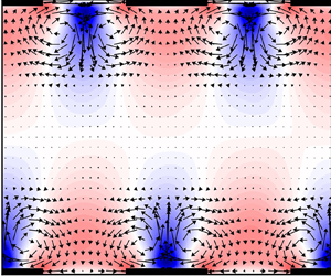
To illustrate the overall flow structure in the heterogeneous simulations, figure 2 shows  $yz$-planes of the temperature (a) and velocity field (b) for case Het-Ri120-pi/2. Figure 2(a) clearly shows the overall stable stratification, since the temperature generally increases with height. Close to the surface, the temperature is seen to be heterogeneous, as prescribed by the boundary conditions. However, we see that further from the walls, the temperature distribution is horizontally homogeneous. As the local surface temperature differences have blended out around
  $z/h = 0.5$, this height can be regarded as the ‘blending height’ for the temperature (Bou-Zeid, Meneveau & Parlange Reference Bou-Zeid, Meneveau and Parlange2004). Due to this spanwise mixing of high and low temperature, the temperature above the cold patches slightly decreases with height. Thus, the local temperature gradient there is negative and convective instability develops locally, as was previously found for streamwise heterogeneous temperature flow (Mironov & Sullivan Reference Mironov and Sullivan2016). The global (mean) temperature gradient is still positive, and will be further discussed in § 3.3.

Figure 2. Contour plots of (a) non-dimensional streamwise- and time-averaged potential temperature $\langle \bar {\theta }\rangle _x /\Delta ^z\theta$ and (b) dispersive velocity deviation
  $\langle \bar {u}''\rangle _x$ normalized with the bulk velocity
  $u_b$, for case Het-Ri120-pi/2. The vectors in (b) represent the in-plane velocity vector (
 $\langle \bar {v}\rangle _x,\langle \bar {w}\rangle _x$). The thick lines on the lower and upper edge in (b) indicate the location of the high surface temperature patches. The spanwise variation of the friction velocity
  $u_\tau$ is plotted with a green line, where the dashed grey line indicates the mean value (1). Note that not the entire domain width is shown.
In figure 2(b) the time-averaged dispersive fluctuation of the streamwise velocity and the in-plane velocity vectors ( $\langle \bar {v}\rangle _x,\langle \bar {w}\rangle _x$) are displayed. The thick lines at the horizontal domain edges indicate the locations where the surface temperature is high
  $(\theta _{b,H}, \theta _{t,H})$, while in between the surface temperature is equal to the lower value
  $(\theta _{b,L}, \theta _{t,L})$. If we focus on the bottom half of the figure, it is clear that there is a strong upward flow in the centre of the high-temperature patches and a weaker downward flow above the low-temperature strips. These mean in-plane vortices can be identified as secondary motions. As a result of the upward transport of low momentum from near the surface, the streamwise velocity is reduced above the high-temperature patches (
 $\langle \bar {u}''\rangle _x < 0$). This velocity deficit reaches up to 35 % of the bulk velocity. Aloft the colder areas, high momentum from the centre of the channel is transported downward resulting in increased streamwise velocity (
 $\langle \bar {u}''\rangle _x > 0$). These so-called HMPs and LMPs are typical for flows with secondary motions, and have been reported in many previous studies with heterogeneous surface roughness (Chung et al. Reference Chung, Monty and Hutchins2018; Forooghi et al. Reference Forooghi, Yang and Abkar2020). However, the magnitude of the reported velocity deficit varies in these studies, e.g. Forooghi et al. (Reference Forooghi, Yang and Abkar2020) found a maximum of only 10 % of the centre velocity
  $u_c$. Regarding the homogeneous case, we point out that
  $\langle \bar {u}'' \rangle _x = 0$ by definition, and no secondary (dispersive) motions are present. Note that this is not in contradiction with often documented streaks in (neutral) homogeneous cases, as these relate to long streamwise structures in the turbulent fluctuating motions described by
  $u'$.
$u'$.
Previous studies into secondary flows induced by spanwise heterogeneous surface roughness emphasized the importance of the imposed spanwise heterogeneity of the wall shear stress (Hwang & Lee Reference Hwang and Lee2018). The friction velocity  $u_\tau = (\nu \partial \langle \bar {u} \rangle _x /\partial z)^{1/2}$ is directly related to the streamwise wall shear stress and is shown by the green line in figure 2(b). We clearly see that the maximum values of the wall shear stress occur at the location of the temperature transition. A similar observation was made by Hwang & Lee (Reference Hwang and Lee2018), where the maximal values of the wall shear stress in flow over elevated strips were located at the edges of the ridges. Away from the transition, we find that the shear stress at the low-temperature strips is larger than at the high-temperature strips.
Comparing the velocity and temperature fields in figure 2, we find that the blending height for the velocity, i.e. the height where the velocity field becomes horizontally homogeneous and, thus,  $\bar {u}''=0$, is higher than for that for the temperature. Furthermore, we notice that the upward motions above the high-temperature strips seem to be maximal in the regions with local convective instabilities. The local unstable stratification can therefore be related to the observation that the upward motions are stronger than the downward motions. Lastly, the spanwise motions near the surface are in the same direction as the spanwise temperature mixing.
Although we only show one case here for brevity, we point out that all simulations with heterogeneous temperature contain qualitatively similar secondary flow patterns. By contrast, in previous studies into secondary flows generated by heterogeneous surface elevation or wall shear stress, the spanwise location of the HMPs and LMPs and rotational sense are an object of ongoing discussion (Stroh et al. Reference Stroh, Schäfer, Forooghi and Frohnapfel2020), as they are significantly influenced by the type of roughness (Hwang & Lee Reference Hwang and Lee2018). In the present simulations, where the secondary flows are generated by heterogeneous surface temperature, the rotational direction of the secondary flows and the spanwise locations of the LMPs and HMPs are consistent over all cases, regardless of the spanwise spacing, Reynolds number or Richardson number; the HMPs always occur above the low-temperature strips, while the LMPs arise above the high-temperature strips. However, the size and strength of the vortices vary between the cases, as will be discussed further below.
3.2. Global skin friction and heat transfer coefficients
In the previous section we demonstrated that spanwise heterogeneous surface temperature induces secondary vortices and heterogeneous mean velocity fields. From previous studies, it is known that secondary motions generated by spanwise height or roughness differences significantly affect momentum and heat transfer (Stroh et al. Reference Stroh, Schäfer, Forooghi and Frohnapfel2020). In the current section we discuss how the skin friction coefficient  $C_f$ and Nusselt number Nu are affected by the heterogeneous surface temperature. To that end, figure 3 gives an overview of these integral flow properties for all inhomogeneous simulations, as a function of the spanwise heterogeneity length scale
  $\lambda /h$. To enable easy comparison between homogeneous and heterogeneous channel flows, the values of
  $C_f$ and Nu are normalized by the corresponding homogeneous simulation with the same Reynolds and Richardson number.

Figure 3. Friction coefficient  $C_f$ (a) and Nusselt number Nu (b) vs surface temperature wavelength for all heterogeneous simulations, normalized by the corresponding homogeneous simulations. Errorbars are bootstrap 95 % confidence intervals as described in § 2.3.
In figure 3(a) it is clear that the friction coefficient peaks at a certain intermediate wavelength, and then for larger  $\lambda$ decreases again towards the corresponding homogeneous value (1 in the graph). This trend is in agreement with results of Chung et al. (Reference Chung, Monty and Hutchins2018) for DNS with spanwise varying wall shear stress, and is strongly related to the size and strength of the secondary motions as discussed in §§ 3.3 and 3.5.2. The most striking observation in figure 3(a) is that for the
  $Re_\tau =550$ simulations,
  $C_f/C_{\textit {f,hom}}$ drops below 1 (green line in figure 3a) for
  $\lambda /h \geq {\rm \pi} /2$. In other words, we find that the skin friction in stably stratified channel flow with heterogeneous temperature walls can be lower than with homogeneous temperature walls for the given Reynolds number of
  $Re_\tau = 550$. The very small size of the errorbars indicates that this difference is indeed significant, and the largest reduction with respect to the homogeneous simulation is approximately 8 % for the
  $\lambda /h = {\rm \pi}$ and
  $2{\rm \pi} $ cases. It is worth noting that Medjnoun et al. (Reference Medjnoun, Vanderwel and Ganapathisubramani2018) also found indications of skin friction reduction for flow over a heterogeneously rough wall compared with a smooth wall at a given Reynolds number, although in their experimental results the difference was of the order of the measurement uncertainty. A further discussion on the observed drag reduction follows in § 3.3.
Besides that, if we compare the Re180 and Re550 curves, we find that the height and wavelength of the  $C_f$ peak is decreased by the increase in Reynolds number. The dependency of
  $C_f$ on both spanwise heterogeneity scale and Reynolds number also agrees with the results of the aforementioned wind-tunnel study of flow over elevated strips by Medjnoun et al. (Reference Medjnoun, Vanderwel and Ganapathisubramani2018). By contrast, for the homogeneous cases, the skin friction coefficient depends on the stability only and not on the Reynolds number (cf. table 1). This is in line with García-Villalba & del Álamo (Reference García-Villalba and del Álamo2011) and Zonta & Soldati (Reference Zonta and Soldati2018)'s findings that
  $C_f \sim Ri_\tau ^{-1/3}$ even for larger Reynolds and Richardson numbers. From the present results it is clear that such a simple relation between skin friction and stability does not hold for thermally heterogeneous flows.
Given the fact that the blue and orange lines overlap for almost all spacings, we can conclude that the in-phase and antiphase configurations result in an equal friction coefficient (and Nusselt number, see figure 3b) for small spacings. For larger  $\lambda /h$, we observe minor differences, which are investigated further in § 3.5.
Regarding strongly stable cases (red lines), we see that the effect of the heterogeneous surface temperature on the friction coefficient and Nusselt number is generally smaller than in the weakly stratified cases. The overall trend of the  $C_f/C_{\textit {f,hom}}$-curve is similar to the Ri120 cases, yet the peak height and surface wavelength at which the friction is maximal are shifted. Moreover, by comparing the absolute values in table 1, we learn that the friction coefficient is strongly reduced by the increased stability, as was found previously in homogeneous stable channel flows (García-Villalba & del Álamo Reference García-Villalba and del Álamo2011). Since
  $u_\tau$ is fixed by the constant pressure gradient in our simulations, the differences in friction coefficient can only be caused by variation in the bulk velocity
  $u_b$, which is again directly related to the bulk Reynolds number
  $Re_b$ (see table 1). Therefore, each of the observations in figure 3(a) can be translated to statements about the bulk Reynolds number and velocity. For example, the difference in
  $u_b$ and
  $Re_b$ between the weakly and strongly stratified case is about a factor 2 (cf. table 1). This acceleration can be ascribed to a decrease in the turbulent and dispersive momentum fluxes as stable stratification damps both turbulent and dispersive wall-normal motions (García-Villalba & del Álamo Reference García-Villalba and del Álamo2011; Forooghi et al. Reference Forooghi, Yang and Abkar2020).
In the following we turn our focus to the dependency of the Nusselt number on the surface temperature wavelength, as displayed in figure 3(b). The Nusselt number characterizes the convective heat transfer at the wall, and can also be used as an indication of how close the temperature profile is to a laminar state. For the Re180 cases, we observe that Nu decreases as  $\lambda /h$ increases. At
  $\lambda /h = {\rm \pi} /2$ there seems to be a local minimum, but at the two largest spacings the values are decreasing again.
Looking at the Re550 cases, we observe that the curve for the Nusselt number has a minimum at the same wavelength as the Re180 curve ( $\lambda /h = {\rm \pi} /2$), and even the values of the relative Nu reduction of the local minima for the Re180 and Re550 curves are very close, at 65 % and 70 % of the homogeneous value, respectively. However, in contrast to the low-Reynolds curves, the Re550 curve seems to recover towards its homogeneous value as the width of the temperature strips increases.
Comparing the non-normalized values of Nu in table 1, it is clear that one effect of increasing the Reynolds number is to increase the Nusselt number and, thus, the wall heat transfer. Another interpretation is that the high-Reynolds flow is further from laminarization than the low-Reynolds flow, as  $\textit {Nu}=1$ for laminar flow.
Lastly, we remark that the red curve in figure 3(b), which represents the effect of the heterogeneous temperature on the wall heat transfer in the very stable simulations with  $Ri_\tau =960$, remains around 1. Hence, we can infer that the wall heat transfer is not much affected by the heterogeneity length scale, or the heterogeneous wall temperature in general. This will be discussed further in § 3.4.
As mentioned before, Stroh et al. (Reference Stroh, Schäfer, Forooghi and Frohnapfel2020) found that both  $C_f$ and Nu increase in the presence of secondary flows induced by streamwise elevated ridges compared with a smooth wall. The enhanced skin friction is consistent with most of the present cases, except for the drag reduction in some high-Reynolds cases. Their reported increase in heat transfer due to secondary motions contradicts our results, which may be related to the fact that they did not take stratification effects into account.
Regarding the ‘missing’ data point for  $Re_\tau = 550$ at
  $\lambda /h = 4{\rm \pi} $, we note that we could not run this case because the spanwise domain size for these simulations was only
  $2{\rm \pi} $. On the same note, one may argue that the results could be dependent on the spanwise domain size, particularly in the cases with the largest spacing, where
  $\lambda /h$ is close or equal to
  $L_y$. To check this, we performed a simulation with
  $Re_\tau = 180, Ri_\tau = 120$ and
  $\lambda /h = 4{\rm \pi} $ (similar to Het-Ri120-4pi) on a domain that was twice as large in the spanwise direction (
 $L_y = 8{\rm \pi} $). The resulting mean profiles of this simulation (not shown) were virtually equal to case Het-Ri120-4pi. Moreover, the difference in
  $C_f$ was within the uncertainty range (<0.5 %), whereas the deviation in Nu was only 2 %. Therefore, we assume that the effect of spanwise domain size on our results is small.
3.3. Effect of Reynolds number
The velocity and temperature fields of the simulations with  $Re_\tau =550$ look qualitatively very similar to those for the Re180 cases in figure 2 and are therefore not displayed here. The main quantitative difference is the magnitude of the velocity deficit, which is maximal 20 % of the bulk velocity (vs 35 % in the low-Reynolds case). As we learned in the previous section, the friction coefficient decreases and the Nusselt number increases at higher Reynolds number. Moreover, if the surface temperature wavelength is larger than the half-channel height (
 $\lambda /h \geq {\rm \pi} /2$), the friction coefficient is lower than for homogeneous stable flow.
3.3.1. The decomposition of  $C_f$ and Nu

To get more insight in the physical reasons behind the trends observed in figure 3, we apply the decomposition of  $C_f$ and
  $Nu$ as described in § 2.3 ((2.11) and (2.12)). The laminar, turbulent and dispersive contributions to the skin friction coefficient and Nusselt number are displayed in figure 4.

Figure 4. Laminar, turbulent and dispersive contribution to the skin friction coefficient (a) and Nusselt number (b), calculated with (2.11) and (2.12), for the heterogeneous simulations with  $Re_\tau =550$,
  $Ri_\tau =120$. The corresponding homogeneous simulation is plotted at
  $\lambda /h = 0$. The total values (red lines with 95 % bootstrap confidence intervals as errorbars) are also plotted for reference.
The laminar contribution, which is proportional to  $Re_b^{-1}$, is almost equal in all simulations, while the other terms clearly depend on the spanwise heterogeneity. As expected, the dispersive contribution is 0 in the homogeneous case. When spanwise high- and low-temperature strips with a small width are introduced, the friction coefficient rises due to an increase in both the Reynolds stress and the dispersive stress. As the spanwise heterogeneity length scale becomes larger, the dispersive contribution keeps increasing, but the turbulent component decreases. Both this increase and decrease seem to be asymptotic in the
  $\lambda /h$ range that was investigated here. Wind-tunnel experiments by Medjnoun et al. (Reference Medjnoun, Vanderwel and Ganapathisubramani2020) also showed that the turbulent stresses in a heterogeneous flow are smaller than in a homogeneous flow. We can conclude that drag reduction with respect to the homogeneous stable channel is caused by a decrease of the turbulent stress that exceeds the rise of the dispersive stress. Yet, the contribution of the dispersive stresses to the skin friction coefficient is significant with approximately 25 % of the total value, but remains more than a factor two smaller than the Reynolds stresses.
Figure 4(b) shows the decomposition of the Nusselt number. Again, the dispersive heat flux is 0 in the homogeneous case and the laminar contribution to the heat flux in all cases is per definition equal to 1. We further remark that the contribution of the dispersive heat flux to the heat transfer is negative, while the contribution of the turbulent heat flux is positive. The latter is inherent to stably stratified flows, where the surface heat flux  $\langle \overline {w'\theta '}\rangle _0$ is per definition negative such that
  $-\langle \overline {w'\theta '}\rangle _0$ is positive. We can explain why the dispersive stress is negative by looking back at figure 2. Since air above the warm temperature patches is moving upwards,
  $\bar {w}'' = \bar {w} - \langle \bar {w} \rangle > 0$ at locations where
  $\bar {\theta }'' = \bar {\theta } - \langle \bar {\theta } \rangle > 0$ (while above the hot patches the opposite holds), we find that
  $-\langle \bar {w}''\bar {\theta }''\rangle$ is negative. Thus, the turbulent transport of warm air downward is counteracted by dispersive heat transport in the opposite direction. The magnitude of the dispersive heat flux increases with
  $\lambda /h$, similar to the dispersive momentum flux in figure 4(a). By contrast, the turbulent heat flux does not have the same
  $\lambda /h$ dependency as the turbulent momentum flux, as it has a minimum at
  $\lambda /h = {\rm \pi} /2$ and then rises again. This increase in turbulent heat flux is larger than the increase of dispersive heat flux in the opposite direction, such that the total Nusselt number increases again for
  $\lambda /h > {\rm \pi} /2$.
3.3.2. Mean profiles
Figure 5(a,b) displays horizontally averaged velocity and potential temperature profiles for the simulations with  $Re_\tau = 550$. The inset in (a) shows that in the viscous sublayer (
 $z^+ < 5$) the classic linear relation
  $u^+ = z^+$ (Pope Reference Pope2000) holds for all simulations. This is obviously due to the fact that constant viscous wall shear (
 $(\nu (\partial \langle \bar {u}\rangle /\partial z)_w)^{1/2} = u_\tau$) is enforced by the streamwise pressure gradient (
 $F_p$ in (2.2)). Further from the wall, the profiles diverge. By comparing the velocities further from the wall, at
  $z/h = 0.25$, we see that the velocity increase near the wall is stronger as
  $\lambda /h$ increases. Moreover, the near-wall velocity gradient for
  $\lambda /h > {\rm \pi} /4$ is larger than for the homogeneous case. By contrast, the centre velocity in homogeneous stable channel flow is clearly larger than for all heterogeneous channels. Despite that, the bulk velocity in the heterogeneous cases with
  $\lambda /h \leq {\rm \pi} /2$ is still larger than in the homogeneous case, which we could already conclude from the friction coefficient plots (figure 3a) or the bulk Reynolds numbers reported in table 1.

Figure 5. (a,b) Horizontally averaged streamwise velocity (a) and potential temperature (b) for the simulations with  $Re_\tau = 550$ and
  $Ri_\tau = 120$. The insets are a zoom of the near-wall region, with the dashed line in (a) representing
  $u^+ = z^+$ and the markers in (b) representing the location of the first three grid points. The horizontal axis in the inset in (a) is scaled in wall units (
 $z^+ = u_\tau z /\nu$). (c,d) Horizontally averaged profiles of turbulent (-, full lines), dispersive (- -, dashed lines) and viscous (-.-, dash-dotted lines) momentum (a) and heat flux (b).
The viscous, turbulent and dispersive components of the vertical momentum flux, as described in (2.9), are presented in figure 5(c). Naturally, the viscous component is dominant in the near-wall region, due to the high velocity gradient there. Moreover, the viscous component at the wall is equal to the friction velocity  $u_\tau = 1$. The sum of all components adds up to a perfectly straight line for the total shear stress, corresponding to
  $u_\tau ^2(1 - z/h)$ (grey dashed line in figure 5c), which indicates the fully developed flow state of all simulations. In the homogeneous case the turbulent momentum flux is larger than in the heterogeneous cases, while the dispersive flux is zero. The viscous stress slightly increases close to the channel centre, as the velocity profile shows a small inclination there.
For the heterogeneous cases, the dispersive momentum fluxes in figure 5(c) show a peak close to the wall, and then decrease again. The location of the peak in the dispersive stresses can be used as a rough estimate for the size of the wall-attached secondary vortices (Forooghi et al. Reference Forooghi, Yang and Abkar2020). Given that the location of the maximal value of  $\langle \bar {u}''\bar {w}''\rangle$ in figure 5(c) increases with
  $\lambda /h$, we conclude that the size of these vortices increases with increasing patch spacing. This is qualitatively consistent with results of Chung et al. (Reference Chung, Monty and Hutchins2018) who studied flow over heterogeneous roughness with varying spanwise spacing. At small
  $\lambda /h$, the secondary motions are confined near the wall, leaving a virtually homogeneous bulk region where dispersive stresses vanish. At intermediate spacings, the size of the vortices increases, until for a certain spacing the heterogeneity has reached the channel centre. Figure 5(c) shows that this occurs in the cases with
  $\lambda /h \geq {\rm \pi}$, where the dispersive momentum flux is non-negligible and even negative in the centre of the channel. Since the viscous contribution is negligible in the channel core, the peaks in the dispersive stress profiles are compensated by decreases in turbulent flux in order to add up to the linear total stress profile. This corroborates the results of Nikora et al. (Reference Nikora, Stoesser, Cameron, Stewart, Papadopoulos, Ouro, McSherry, Zampiron, Marusic and Falconer2019), who also found an interdependence between the contributions of turbulent and dispersive stresses in their analysis of flow over roughness beds (i.e. an increase in one may lead to a decrease in the other). Moreover, these trends are consistent with the decrease in the turbulent contribution to the friction coefficient that was observed in figure 4(a). Furthermore, the fact that the dispersive flux can be of almost the same size as the turbulent flux highlights the role of secondary motions in momentum transport.
The horizontally averaged temperature profiles are displayed in figure 5(b). We observe high temperature gradients close to the wall, characterizing a strong stably stratified boundary layer that inhibits vertical temperature transport at the wall (Armenio & Sarkar Reference Armenio and Sarkar2002). After a region where the temperature gradient is more or less constant, another layer with a high temperature gradient (a pycnocline) is formed near the channel centre. The extent and strength of the near-wall temperature boundary layer and pycnocline in the centre are strongly affected by the heterogeneity length scale. If we compare the temperatures at  $z/h = 0.4$, the temperature is higher as
  $\lambda /h$ increases, and, thus, the mean temperature gradient increases with
  $\lambda /h$. This may seem to be in contradiction with figure 3(b), where we found that the Nusselt number in the heterogeneous flows is lower than in the homogeneous case. Given the definition of the Nusselt number in (2.5), it is merely a measure of the temperature gradient at the wall. The inset in figure 5(b) shows the temperature in the first three off-wall grid points, and there it is indeed clear that the wall temperature gradient in the homogeneous case is larger than in the heterogeneous cases. However, we conclude that the strength of the temperature boundary layer is apparently not directly correlated to the Nusselt number, in contrast to homogeneous stable channel flows where the strength of the near-wall pycnocline and the Nusselt number both decrease with increasing stability (García-Villalba & del Álamo Reference García-Villalba and del Álamo2011).
In order to investigate this further, we can look at the different components of the vertical heat flux (cf. (2.10)), as presented in figure 5(d). By applying the triple composition to the temperature transport equation (2.3) and integrating once from 0 to  $h$ with the appropriate boundary conditions, it can be shown that the total heat flux
  $q_z$ is constant through the channel (Armenio & Sarkar Reference Armenio and Sarkar2002). Since the turbulent fluxes vanish at the wall, this constant value is equal to the molecular flux at the wall, i.e.
 \begin{equation} q_z = \left(\alpha\frac{{\textrm d}\langle \bar{\theta}\rangle}{{\textrm d}z}\right)_w=\underbrace{\alpha\frac{{\textrm d}\langle \bar{\theta}\rangle}{{\textrm d}z}}_{\textit{viscous}} -\underbrace{\langle \overline{w'\theta'} \rangle}_{\textit{turbulent}} -\underbrace{\langle \bar{w}''\bar{\theta}''\rangle}_{\textit{dispersive}}. \end{equation}
Because, the temperature gradient at the wall is directly related to the Nusselt number in our simulations (2.5), Nu could be regarded as a direct measure for the constant value of the heat flux through the entire channel.
In figure 5(d) we observe that the temperature gradient in the heterogeneous simulations increases sharply close to the wall, while for the homogeneous case, the temperature gradient at the wall is the maximal temperature gradient. Equation (3.1) shows that the temperature gradient can only exceed the wall value if the combined contribution of the turbulent and dispersive fluxes is negative. Figure 5(d) demonstrates that near the wall, the dispersive heat flux dominates the turbulent heat flux and is indeed negative. This also agrees with the negative dispersive contribution to the Nusselt number as observed in figure 4 and discussed above. In line with the dispersive momentum flux, the height of the (absolute) maximum in the dispersive heat flux increases with increasing  $\lambda /h$. By contrast, the value of the maximum seems to decrease for larger spacing, while the integrated area increases, which corresponds again to the dispersive contribution to the Nusselt number displayed in figure 4(b). Therefore, we can conclude that the secondary motions play an important role in the temperature distribution near the wall.
Conversely, the dispersive heat flux is negligible in the core of the channel, where the turbulent heat flux prevails. García-Villalba & del Álamo (Reference García-Villalba and del Álamo2011) showed that for homogeneous strongly stratified flow ( $Ri_\tau \geq 480$ at
  $Re_\tau = 550$), the turbulent heat flux in the centre of the channel is reduced to approximately zero such that the mean density gradient at the centre equals the mean density gradient at the wall. In the present heterogeneous simulations the turbulent heat flux in the centre is larger than in the homogeneous simulation, which explains why the temperature gradient in the centre is smaller.
Lastly, we remark that Vanderwel et al. (Reference Vanderwel, Stroh, Kriegseis, Frohnapfel and Ganapathisubramani2019) found that DNS at  $Re_\tau = 500$ and wind-tunnel experiments at
  $Re_\tau = 4000$ of roughness-induced secondary flows under neutral stratification produce similar results in the mean flow as well as the dispersive and turbulent stress distributions, and that the energetic aspects of the secondary motions are not very sensitive to the Reynolds number. Therefore, we may assume that the findings in our Re550 cases can be extended to higher Reynolds numbers, but this should be further verified in the future.
3.4. Effect of strong stability
We now discuss the strongly stratified simulations with  $Ri_\tau =960$ and compare them to the moderately stable Ri120 simulations.
Figure 6 provides an overview of the temperature and velocity distributions for case Het-Ri960-pi/2, where we only show the lower half for clarity. If we compare this figure to the Ri120 case in figure 2, it is clear that increasing the stability of the flow significantly affects the vertical extent of the heterogeneity and the vortices. This observation is in agreement with Forooghi et al. (Reference Forooghi, Yang and Abkar2020), who also concluded that stable stratification reduces the vertical size and strength of the roughness-induced secondary flows. Moreover, they observed secondary and tertiary vortices on top of the vortices closest to the wall as the stability increases. Although this is not clearly visible in figure 6(b), we also observed this ‘vortex stacking’ in our simulations with  $Ri_\tau =960$.

Figure 6. Contour plots of (a) streamwise- and time-averaged non-dimensional potential temperature  $\langle \bar {\theta } \rangle _x/\Delta ^z\theta$ and (b) dispersive velocity deviation
  $\bar {u}''$ normalized with the bulk velocity
  $u_b$, for case Het-Ri960-pi/2. The vectors in (b) represent the in-plane velocity vector (
 $\langle \bar {v} \rangle _x, \langle \bar {w} \rangle _x$). The thick lines on the lower edge in (b) indicate the location of the high surface temperature patches. The spanwise variation of the friction velocity
  $u_\tau$ is plotted with a green line, where the dashed grey line indicates the mean value (1). Note that only the lower channel half and not the entire domain width is shown.
Due to the reduced vertical extent of the vortices, the blending height of the streamwise velocity is also lowered such that  $u$ is nearly homogeneous in the bulk of the channel. Furthermore, the vectors show that the spanwise velocity is larger than the vertical velocity, indicating that mainly the vertical motions are reduced by the stable stratification. The dispersive velocity fluctuation is not larger than 15 % of the bulk velocity, while it was 35 % in the Ri120 case. Besides that, the spanwise variation of the friction velocity (and wall shear stress), displayed by the green line in figure 6(b), is comparable to the moderately stable case, except that the minima of
  $u_\tau$ in the Ri960 case are slightly higher.
Analogous to the comparison of the velocity fields, the temperature plotted in figure 6(a) is also less inhomogeneous than in the Ri120-Re180 case (figure 2a). Moreover, the horizontal temperature difference relative to the vertical temperature difference,  $\Delta ^y\theta /\langle \Delta ^z\theta \rangle$, at the lower boundary is smaller than in the moderately stable cases. As explained in § 2.2, this reduced surface temperature amplitude was prescribed by the boundary conditions, in order to keep the horizontal buoyancy difference (
 $Ri_\tau \theta ''$) at the surface and the horizontal Richardson number
  $Ri_\tau ^y$ equal to the Ri120 cases. We note here that we also performed preliminary simulations where both
  $Ri_\tau ^z$ and
  $Ri_\tau ^y$ were increased by keeping the surface temperature amplitude
  $\Delta ^y\theta$ equal to the cases with
  $Ri_\tau ^z$. This resulted in vortex sizes comparable to the Ri120 simulations, but further analysis of this configuration was not performed and could be included in future research.
From decomposition of the vertical momentum and heat fluxes (not shown), we infer that the dispersive contributions in the strongly stable cases are much smaller than in the moderately stable cases. Combined with the findings of smaller streamwise velocity deficits and smaller changes in  $C_f$ and
  $Nu$, this leads to the conclusion that the importance and strength of the secondary motions is reduced by increased stability.
3.4.1. Laminarization and intermittent turbulence
For homogeneous stable channel flow, it is known that increasing the stability reduces turbulence levels and, thus, turbulent heat and momentum transport (Zonta & Soldati Reference Zonta and Soldati2018). Therefore, it can be anticipated that the Nusselt number and skin friction coefficient are reduced by increasing the stability, as the flow is closer to laminarization. The Nusselt number for our Ri960 simulations is around 1.3 (cf. table 1), so not completely laminar yet, and figure 3 showed that it is not much affected by the heterogeneity length scale of the surface temperature.
However, a crucial remark here is that according to the linear stability theory from Gage & Reid (Reference Gage and Reid1968), the critical value of  $Ri_\tau$ above which a homogeneous channel flow at
  $Re_\tau = 180$ should be completely laminar is
  $Ri_\tau \approx 900$ (Armenio & Sarkar Reference Armenio and Sarkar2002). Therefore, our Ri960 cases would be expected to be in the strongly stratified laminar regime (see also figure 4 in Zonta & Soldati Reference Zonta and Soldati2018). Nevertheless, in the present simulations neither the homogeneous nor the heterogeneous simulations become completely laminar. This may be related to the fact that our Ri960 simulations were initialized from a laminar profile with very large velocities and large artificial turbulent perturbations, while previous DNS studies of stable channel flow (Garg et al. Reference Garg, Ferziger, Monismith and Koseff2000; García-Villalba & del Álamo Reference García-Villalba and del Álamo2011; He & Basu Reference He and Basu2016; Atoufi et al. Reference Atoufi, Scott and Waite2020) initialized their strongly stable cases from a fully developed realization of a previous neutral or even stably stratified simulation. Hence, the initial flow velocity and turbulence level in our Ri960 simulations are much higher than in these DNS studies. We remark that if we initialize our Ri960 simulations in the same way, from a fully developed neutral or stable flow field, the flow indeed becomes laminar immediately after initialization. However, if we keep these simulations running for a long enough time, the flow keeps accelerating and shear keeps building up, until turbulence is regenerated. This development matches with the conclusion of Donda et al. (Reference Donda, van Hooijdonk, Moene, Jonker, van Heijst, Clercx and van de Wiel2015) that turbulence collapse is only temporary.
Previous studies have demonstrated that strongly stratified flows with intermittent turbulence show turbulent bursting events in their time evolution, while instantaneous horizontal planes show coexisting laminar and turbulent patches (García-Villalba & del Álamo Reference García-Villalba and del Álamo2011; Brethouwer et al. Reference Brethouwer, Duguet and Schlatter2012; He & Basu Reference He and Basu2015). An inspection of the time evolution of  $C_f$ and Nu in our Ri960 cases, as shown in figure 7, reveals that indeed large fluctuations are present in these values. The magnitude of the fluctuations, or even sharp peaks, is greatest in the Het-Ri960-pi/8, Het-Ri960-4pi and Hom-Ri960 simulations, which are also expected to be closest to homogeneous flows as they are in the
  $\lambda /h \ll 1$ and
  $\lambda /h \gg 1$ regimes. For the intermediate spacings (
 ${\rm \pi} /4 \leq \lambda /h \leq 2{\rm \pi} $), the fluctuations are significantly smaller. These low-frequency oscillations are similar to those reported by García-Villalba & del Álamo (Reference García-Villalba and del Álamo2011) and Brethouwer et al. (Reference Brethouwer, Duguet and Schlatter2012), who attributed this to a (too) small domain size.

Figure 7. Time evolution of  $C_f$ (a) and Nu (b) over the averaging period between
  $tu_\tau /h = 60$ and
  $tu_\tau /h = 90$.
Following He & Basu (Reference He and Basu2015), we illustrate the temporal variability of intermittent turbulence across the entire channel by means of time-height plots of the square of the instantaneous vertical velocity fluctuation in figure 8. Here  $w'' = w-\langle w \rangle$ denotes the instantaneous dispersive deviation from the horizontal average, but we remark that
  $w'' = w' = w$ because the time and horizontal averages
  $\langle w \rangle$ and
  $\bar {w}$ are per definition zero due to the boundary conditions. High values of
  $\langle w''w'' \rangle$ can be interpreted as turbulent bursting events, while low values represent laminar flow states. Qualitatively, it is clear that the variability in the homogeneous case (figure 8a) is larger than in the heterogeneous case (figure 8b). At the bottom of the domain,
  $\langle w''w'' \rangle$ reduces to zero as a result of the constraint of the boundary conditions (
 $w =0$). In the centre of the channel the velocity fluctuation is also very small, indicating that the channel core is close to the laminar state. Vertical profiles of these cases (as in figure 5, not depicted here for brevity) show that this laminar core region is in addition characterized by high velocity and temperature gradients, while the vertical momentum and temperature fluxes are small. The lack of vertical transport in the channel centre leads to a decoupling of the two channel halves, as previously found by Garg et al. (Reference Garg, Ferziger, Monismith and Koseff2000), Iida et al. (Reference Iida, Kasagi and Nagano2002) and García-Villalba & del Álamo (Reference García-Villalba and del Álamo2011). This decoupling is illustrated most clearly in figure 8(a), where, for example, at
  $tu_\tau /h = 80$ the lower channel is in a phase with high turbulence intensity, while the turbulence level in the upper channel is much lower.

Figure 8. Time-height plots of square instantaneous vertical velocity profiles over the averaging period between  $t^* = 60$ and
  $t^* = 90$. (a) The homogeneous case with
  $Ri_\tau = 960$ and
  $Re_\tau = 180$, (b) the heterogeneous case with
  $Ri_\tau = 960$ and
  $Re_\tau = 180$ and
  $\lambda /h = {\rm \pi} /2$.
From the discussion above, we may conclude that strongly stratified flow with heterogeneous surface temperature in the range  $\lambda /h \approx 1$ is less likely to express intermittent turbulence than very stable homogeneous flow. Or, in other words, the critical stability for which stable channel flow becomes laminar is higher for heterogeneous channels compared with homogeneous channels. This is in line with wind-tunnel results from Williams et al. (Reference Williams, Hohman, Van Buren, Bou-Zeid and Smits2017), where turbulence collapse occurred at a bulk Richardson number of 0.1 for smooth walls and 0.15 for rough walls. In contrast, Flores & Riley (Reference Flores and Riley2011) found
  $Re_L = L_{MO}u_\tau /\nu \approx 100$ as a critical value for turbulence collapse, and state that this can be extended to rough surfaces. In the present Ri960 cases, this so-called Obukhov-Reynolds number can be calculated from the values in table 1, with
  $Re_L = Re_\tau / (h/L_{MO}) \approx 90$. The fact that turbulence has not fully collapsed in the present simulations indicates that Flores & Riley's
  $Re_L$ criterion does not hold for spanwise heterogeneous flows.
To examine the spatial variability of the turbulence, figure 9 shows horizontal planes of the instantaneous vertical velocity  $w''$, located at
  $z^+ = 15$ (
 $z/h = 0.083$). For homogeneous very stable channel flow, it is known that laminar and turbulent patches coexist near the wall, illustrated by areas with strong and weak vertical velocity (He & Basu Reference He and Basu2015). Figure 9(d) shows that for the homogeneous case with moderate stability, oblique ‘bands’ of laminar and turbulent patches occur, while for very stable flow (figure 9b), the turbulent patches are smaller and less organized, indicating that the flow is closer to laminarization (García-Villalba & del Álamo Reference García-Villalba and del Álamo2011; Brethouwer et al. Reference Brethouwer, Duguet and Schlatter2012). In the strongly stratified Het-Ri960-pi/2 case, depicted in figure 9(a), we still observe areas with high and low vertical velocity, but on the background we clearly see the footprint of the heterogeneous surface temperature. For the moderately stable heterogeneous case (figure 9c), the banded pattern from the homogeneous case has disappeared, and the vertical velocity is governed by the high- and low-temperature patches. That is,
  $w$ is predominantly upward and downward aloft the respective high- and low-temperature strips, which are indicated by the varying line width on the domain boundaries in figure 9(a,c). Thus, we find that the heterogeneous surface temperature breaks the pattern of laminar and turbulent patches near the wall.

Figure 9. Instantaneous contours at  $tu_\tau /h = 90$ of the vertical velocity deviation
  $w''$ at a horizontal
  $x$–
$x$– $y$ plane located at
  $z^+ = 15$ (
 $z/h = 0.083$). Plots (a) and (c) are heterogeneous cases with
  $\lambda /h = {\rm \pi} /2$ and
  $Ri_\tau = 960$ and 120, respectively, where the thick lines on the left and right edges indicate the location of the high surface temperature patches. Plots (b) and (d) are homogeneous cases with
  $Ri_\tau = 960$ and 120, respectively.
3.5. Effect of upper wall temperature phase
Lastly, we study the difference between the in-phase and antiphase upper temperature boundary conditions. In all the previously discussed simulations, the square wave that defines the upper surface temperature was in phase with the bottom temperature. In addition, we consider a set of simulations where the upper surface temperature is in antiphase with the bottom (cf. figure 1). Figure 10 displays the time- and streamwise-averaged potential temperature (a) and dispersive velocity fluctuation (b) for case Het-Ri120-pi/2-A. In the temperature field we see that a low-temperature patch at the bottom is opposed by a high-temperature patch at the top. Therefore, the local temperature difference there, and thus stability, is double the average value. In between these regions with double stability, the lower- and upper-surface temperatures are equal, and, thus, this region can be considered neutral. However, the temperature field in figure 10(a) shows that the respective low- and high-temperature patches at the bottom and top mix in the spanwise direction, which was already pointed out for the in-phase configuration. As a result, the channel core only ‘feels’ a positive temperature gradient and, thus, stable stratification.

Figure 10. Contour plots of (a) streamwise- and time-averaged non-dimensional potential temperature  $\langle \bar {\theta } \rangle _x/\Delta ^z\theta$ and (b) dispersive velocity deviation
  $\langle \bar {u}''\rangle _x$ normalized with the bulk velocity
  $u_b$, for case Het-Ri120-pi/2-A. The vectors in (b) represent the in-plane velocity vector (
 $\langle \bar {v} \rangle _x,\langle \bar {w} \rangle _x$). The thick lines on the lower and upper edge in (b) indicate the location of the high surface temperature patches. The spanwise variation of the friction velocity
  $u_\tau$ is plotted with a green line, where the dashed grey line indicates the mean value (1). Note that not the entire domain width is shown.
Comparing the temperature fields of the two different configurations (see figure 2a), we find that the temperature blending height is equal for both cases, around  $z/h = 0.5$. In fact, the lower half looks exactly similar, only the upper half of the channel is shifted by a half-phase.
The same holds for the velocity fields in figures 2(b) and 10(b), where a similar shift is observed in the upper channel half. As a result, the HMPs and LMPs in the antiphase configuration are vertically aligned and extend until the channel centre. The streamwise velocity in the channel centre is slightly heterogeneous, and both channel halves seem to be ‘coupled.’ In contrast, the symmetric temperature field in the default configuration in figure 2 results in an antisymmetric velocity field where the streamwise velocity is homogeneous along the channels middle axis. We further observe that the lateral distribution of the friction velocity, indicated by the green line, is equal for both configurations.
3.5.1. Vortex interaction
As mentioned in § 3.2 and demonstrated in figure 3, the integral flow properties of the two different configurations are equal for  $\lambda /h < {\rm \pi}$. To examine the differences at larger spacings, figure 11 displays velocity fields of the in-phase (a) and antiphase (b) cases with
  $\lambda /h = 4{\rm \pi} $. We notice that the vertical size of the secondary motions has increased with respect to the cases with
  $\lambda /h = {\rm \pi} /2$, and the streamwise velocity is heterogeneous in the entire channel. In the antiphase configuration (figure 11a) the upward motions above the high-temperature patches are opposed by downward motions in the upper channel half. In contrast, in the default configuration (figure 11b) the upward motions above the centre of the high-temperature patches are not counteracted in the upper channel half. In this case, the spanwise motions are arranged in such a way that large vortices around the channel centreline appear, and the vortices seem to enhance each other. In the antiphase configuration the mean spanwise velocities around the channels centreline are in the same direction.

Figure 11. Contour plots of streamwise- and time-averaged dispersive velocity deviation  $\langle \bar {u}''\rangle _x$ normalized with the bulk velocity
  $u_b$, for cases with surface temperature in-phase (Het-Ri120-4pi, a) and in antiphase (Het-Ri120-4pi-A, b). The vectors represent the in-plane velocity vector (
 $\langle \bar {v}\rangle _x,\langle \bar {w}\rangle _x$). The thick lines on the lower and upper edge indicate the location of the high surface temperature patches. The spanwise variation of the friction velocity
  $u_\tau$ is plotted with a green line, where the dashed grey line indicates the mean value (1).
Besides, figure 11(a,b) reveals significant differences in the location and size of the maximal dispersive streamwise velocity. The deviation from the horizontal mean velocity is up to 30 % of  $u_b$ in the default configuration, while it is only 17 % in the antiphase configuration. The spanwise location of the largest velocity deficit in figure 11(a) is in the centre of the low-temperature patch, at the edges of the domain. In the other configuration (b), the minimal velocity deficit occurs around halfway between the centre and the edge of the high-temperature patch.
Lastly, we notice subtle differences in the spanwise distribution of the friction velocity of the two configurations, presented by the green lines in figure 11. The minimum value, which occurs at the centre of the low-temperature strip, is lower in the antiphase configuration (figure 11b), while the maximum value, which occurs at the centre of the high-temperature strip, is higher. Furthermore, compared with the cases with  $\lambda /h = {\rm \pi} /2$ in figures 2(b) and 10(b), we see that the locations of the minimal and maximal wall shear stress are reversed. That is, for
  $\lambda /h = {\rm \pi} /2$, the wall shear stress at the high-temperature strips is smaller than at the low-temperature strips, while for
  $\lambda /h = 4{\rm \pi} $, the wall shear stress at the high-temperatures strips is larger than at the low-temperature strips. Moreover, in figure 11 we observe weak HMPs and LMPs very close to the wall, which are opposite in sign compared with the ‘main’ HMPs and LMPs further from the wall. This suggests that, for large
  $\lambda /h$, additional near-wall motions arise, which behave differently from the
  $\lambda$-scale secondary flows in the cases with smaller strip spacings.
3.5.2. Decomposition of velocity and temperature fields
In a previous study, Stroh et al. (Reference Stroh, Schäfer, Forooghi and Frohnapfel2020) studied momentum and heat transfer in a neutral channel with secondary motions induced by streamwise ridges, and they also considered a ‘symmetric’ and a ‘staggered’ arrangement of the ridges. They found only small dissimilarities between the integral flow properties in both configurations, but more significant differences in the composition of the skin friction coefficient and Stanton number. Figure 12 allows us to compare the decomposition of the friction coefficient and Nusselt number between the cases with a different upper temperature boundary condition and  $Re_\tau =180$. The decomposition is again based on (2.11) and (2.12). Interestingly, the total skin friction for
  $\lambda /h$ =
  $2{\rm \pi} $ is equal for both configurations, but its composition is different. In the cases with the largest spacing, both the total value and its components are different. That is, the dispersive contribution is reduced in the antiphase configuration, while the turbulent contribution rises. Because the increase of the turbulent stress exceeds the decrease of the dispersive stress, the total skin friction is higher in the antiphase case, and, thus, the bulk velocity is lower. The absolute value of the dispersive contribution to the heat transfer is also smaller for the antiphase configuration. Profiles of the dispersive and turbulent fluxes (similar to figure 5, not shown here for brevity) reveal the same trends. The decrease of the dispersive contributions indicates that the strength of the vortices and, thus, the role of the secondary motions is reduced in the antiphase configuration, which is related to the smaller streamwise velocity deficit in figure 10(b).

Figure 12. Laminar, turbulent and dispersive contribution to the skin friction coefficient (a) and Nusselt number (b), calculated with (2.11) and (2.12), for the heterogeneous simulations with  $Re_\tau =180$,
  $Ri_\tau =120$. The full and dashed lines indicate the respective in-phase and antiphase configuration. The corresponding homogeneous simulation is plotted at
  $\lambda /h = 0$. The total values (red lines with 95 % bootstrap confidence intervals as errorbars) are also plotted for reference.
More generally, we notice that the dispersive contribution at intermediate spacings is almost of the same magnitude as the turbulent contribution, and the peak in  $C_f$ is caused by enhanced turbulent and dispersive stress. The peak of the dispersive contribution at intermediate spacings is consistent with the findings that the importance of secondary flows induced by spanwise heterogeneous surface roughness is maximal if the spacing is of the order of the boundary layer height (Medjnoun et al. Reference Medjnoun, Vanderwel and Ganapathisubramani2018). Comparing the low-Reynolds cases in figure 12(a) to the decomposition of the cases with
  $Re_\tau = 550$ (§ 3.3.1, figure 4a), we clearly see that the laminar contribution to the friction coefficient is about a factor four higher than in the high-Reynolds cases. The turbulent and dispersive contributions are also larger in the low-Reynolds cases, resulting in an overall larger skin friction.
The contribution of the dispersive heat flux to the Nusselt number follows the same trend as for the Re550 cases in figure 4(b), but is approximately half the magnitude, while the turbulent contribution is also reduced to approximately the same values as the laminar contribution (i.e. 1). Thus, in flows with a low Reynolds number (i.e. low velocity or high viscosity), the turbulent heat flux is too small to cancel out the negative contribution of the dispersive heat transport such that the total Nusselt number decreases as  $\lambda /h$ increases.
4. Conclusions
This study aimed at determining the effect of spanwise heterogeneous surface temperature on stably stratified channel flow using DNS. To that end, the surface temperature was prescribed as a square wave with varying wavelength, while a constant mean temperature difference between the upper and lower wall was maintained. We specifically looked at the influence of the spanwise heterogeneity scale, Reynolds number, stability and upper boundary condition on the mean flow structure and integral flow properties.
In the presence of surface temperature heterogeneity, secondary flows are generated in the plane perpendicular to the flow direction, similar to the secondary motions that are known to be induced by heterogeneous surface roughness. Above the high-temperature regions, the mean flow is upwards under local convective conditions, while above the low-temperature patches the vertical velocity points downward. The secondary motions alter the mean streamwise velocity, forming LMPs above the warm areas and HMPs above the colder areas, with horizontal velocity variations up to 35 % of the bulk velocity.
We showed that the skin friction and heat transfer are significantly affected by the flow heterogeneity, but the exact effect is strongly dependent on the Reynolds number, stability and surface temperature wavelength. Comparison with the corresponding homogeneous stable channel flow revealed that skin friction can be more than doubled in the low-Reynolds cases, while a drag reduction was found for the high-Reynolds number cases when the spanwise temperature length scale exceeded the channel height. In all heterogeneous cases, the wall heat transfer, characterized by the Nusselt number, was lower than in the corresponding homogeneous cases.
Triple decomposition of the velocity and temperature fields allowed the examination of the surface heterogeneity effects through the laminar, turbulent and dispersive stresses. For the high-Reynolds cases, it was found that the dispersive stress, and its contribution to the skin friction, increases as the surface temperature wavelength increases, while the turbulent stress is reduced. As the decrease in turbulent stress becomes larger than the increase in dispersive stress, the skin friction coefficient eventually decreases below the homogeneous value for  $\lambda /h \geq {\rm \pi} /2$. Even though the bulk velocity in these heterogeneous cases is larger than in the homogeneous case, due to more vertical mixing in the core, mean velocity profiles showed that the velocity in the centre of the heterogeneous channels remains lower than in a homogeneous channel. Mean temperature profiles showed that a strong pycnocline is formed near the heterogeneous surface, inhibiting heat transfer. The dispersive heat flux was found to be negative near the wall, and, thus, counteracts the positive turbulent heat flux. Given the size of the dispersive fluxes relative to the other components, we concluded that the secondary motions play an important role in the temperature and velocity distribution.
To study the effect of strong stability, an additional set of simulations was performed, where the vertical Richardson number  $Ri_\tau ^z$ was multiplied with a factor eight while the spanwise buoyancy difference, characterized by
  $Ri_\tau ^y$, remained equal. We showed that the vertical size of the secondary vortices was reduced with respect to the moderately stable cases, and additional weaker vortices were formed on top of the wall-adjacent vortices. Compared with the moderately stable cases, the dispersive fluxes and velocity deficits are smaller and the dependency of the skin friction and Nusselt number on the heterogeneity length scale is weaker. Therefore, we conclude that the importance and strength of the secondary motions is reduced by increased stability. Based on an analysis of the time evolution of the integral flow properties and vertical velocity fluctuation and comparison to a homogeneous strongly stable simulation, we demonstrated that intermittent turbulence and turbulence collapse is less likely to occur in heterogeneous channels with equally strong stratification. Besides, the pattern of laminar and turbulent patches in horizontal planes near the wall, that is known to appear in homogeneous stable channels, is disturbed by the heterogeneous surface.
Lastly, we studied the effect of a phase shift in the square wave that prescribes the upper wall temperature. We found that, for a small temperature patch width, the in-phase and antiphase configurations resulted in equal flow properties. For larger spacing ( $\lambda /h \geq {\rm \pi}$), the secondary motions reach the channel centre, and the vortices in the lower and upper half of the channel interact differently in both configurations. If the lower and upper temperature are in phase, the vortices reinforce each other, leading to larger dispersive and smaller turbulent fluxes than in the antiphase case.
In summary, the present work shows that secondary flows are not only induced by spanwise heterogeneous surface roughness, but also by spanwise heterogeneous surface temperature. In most of the considered cases, these heterogeneities have a significant influence on mean flow properties and, therefore, temperature heterogeneities should not be neglected in surface parametrization models. The exact effect of the heterogeneity on the flow is dependent on many parameters, including the spanwise length scale of the heterogeneity, the Reynolds number, the stability and the upper boundary conditions. More data points are needed to find general trends, through simulations in a wider range of Reynolds and Richardson numbers and spacings. Furthermore, the role of the surface temperature difference and the type of boundary conditions should be examined further. Many variations are possible here, such as a fixed heat flux or cooling rate instead of fixed temperature, a sinusoidal surface temperature pattern instead of a square wave, or a half-channel rather than a full channel. Besides, a fixed pressure gradient is applied as the driving force in the present simulations, while a geostrophic forcing, which induces a height-dependent wind direction, is more relevant for the ABL. These are all interesting topics for future research.
Acknowledgements
The computational resources and services used in this work were provided by the VSC (Flemish Supercomputer Center), funded by the Research Foundation - Flanders (FWO) and the Flemish Government. Furthermore, the authors would like to thank the anonymous reviewers for the insightful comments and pertinent observations made on this work.
Funding
The authors acknowledge support from the Research Foundation Flanders (T.B., FWO grant number G098320N).
Data availability statement
The data that support the findings of this study can be provided by contacting the corresponding author.
Declaration of interests
The authors report no conflict of interest.
Author contributions
T.B. performed code implementations and carried out the simulations in the current work. T.B. and J.M. jointly wrote the manuscript.
Appendix A. Code validation for homogeneous stable channel flow
To verify SP-wind for homogeneous neutral and stably stratified channel flow, we performed a set of simulations similar to that of García-Villalba & del Álamo (Reference García-Villalba and del Álamo2011) and compare the results. Simulation specifications are given in table 1 and 2. The mean profiles of the streamwise velocity, temperature, momentum and heat flux from our simulations are compared in figures 13 and 14, for the cases with  $Re_\tau =180$ and
  $Re_\tau =550$, respectively. As reference, we use data that was extracted with a digitizer from the plots reported by García-Villalba & del Álamo (Reference García-Villalba and del Álamo2011) (GVA2011 in the legends). An important difference between our simulations and the reference GVA2011 simulations is the domain size, which was
  $8{\rm \pi} \times 4{\rm \pi} $ (Re180) and
  $4{\rm \pi} \times 2{\rm \pi} $ (Re550) in the present study, while GVA2011 used
  $18{\rm \pi} \times 8 {\rm \pi}$ (Re180) and
  $8{\rm \pi} \times 3{\rm \pi} $ (Re550) for their stably stratified simulations. Moreover, their code integrates the governing equations in a velocity–vorticity formulation while we use the traditional form of the Navier–Stokes equations (see § 2). Lastly, we use a fourth-order finite-difference scheme in the wall-normal direction, while GVA2011 applies Chebyshev polynomials.

Figure 13. Wall-normal profiles (a) mean velocity, (b) mean temperature, (c) vertical momentum flux and (d) vertical heat flux, for averaged in time and over the horizontal direction. Results from homogeneous stable channel simulations with SP-wind (full coloured lines) are compared with results from García-Villalba & del Álamo (Reference García-Villalba and del Álamo2011) (open symbols) for  $Re_\tau = 180$ and
  $Ri_\tau = 0$, 120, 480. Normalization is in wall variables
  $u_\tau$ and
  $\theta _\tau$.

Figure 14. Same as figure 14, but for simulations with  $Re_\tau =550$. Temperature is normalized by the vertical temperature difference
  $\Delta \theta$ instead of the friction temperature
  $\theta _\tau$.
Despite all these differences, one can see in figures 13 and 14 that the results of the current code (SP-wind) agree very well with those from GVA2011 for all cases. Moreover, the values of the global flow properties reported in table 1 match those of GVA2011 (their table 1). We can conclude that the current solver accurately simulates the mean and turbulent components of neutral and stably stratified channel flow.


