


1. Introduction
Since the seminal work by Kim & Adrian (Reference Kim and Adrian1999), large-scale coherent structures in wall flows have been broadly classified and referred to as large-scale motions (LSMs) and very-large-scale motions (VLSMs). There is now wide consensus about the fact that LSMs typically occur as structures with a longitudinal wavelength of a few outer lengths of the flow  $\delta$ (typically (2–3)
 $\delta$), whereas VLSMs have a wavelength of approximately 10
 $\delta$ or more (Marusic et al. Reference Marusic, McKeon, Monkewitz, Nagib, Smits and Sreenivasan2010). Much less consensus has been reached with respect to the mechanism underpinning the formation of LSMs and VLSMs, which is still elusive and the subject of an ongoing debate. Within this context, two plausible mechanisms are proposed in the literature and are briefly summarized as follows.
Adrian and co-workers support the idea that wall turbulence is dictated by the existence of an omega shaped ‘building-block’ eddy structure, which is often referred to as a hairpin eddy. According to Adrian's view, hairpins can undergo an auto-generation mechanism leading to the formation of packets, which can be interpreted as LSMs. A less clear picture is provided for the generation mechanism of VLSMs, for which Adrian has provided a wide range of plausible hypotheses, among which the preferred one sees VLSMs as a concatenation of LSMs (Adrian Reference Adrian2007).
Cossu, Hwang and co-workers – hereafter referred to as CH – provide a rather different view (for a review, see Cossu & Hwang Reference Cossu and Hwang2017). In a nutshell, they argue that the existence of LSMs and VLSMs is the result of a so-called outer-layer cycle that is independent of the existence of a ‘building-block’ turbulent structure, i.e. hairpins. These authors argue that such an outer-layer cycle shares strong similarities with the well-known near-wall cycle, which was identified 30 years ago as the engine behind turbulence in the buffer zone of wall flows (see e.g. Kim, Kline & Reynolds Reference Kim, Kline and Reynolds1971; Jimenez & Moin Reference Jimenez and Moin1991; Hamilton, Kim & Waleffe Reference Hamilton, Kim and Waleffe1995; Waleffe Reference Waleffe1997). As per the near-wall cycle, the proposed outer-layer cycle involves the existence of low and high (longitudinal) momentum streaks associated with the occurrence of elongated vortices with streamwise vorticity. Such low and high momentum streaks are very long and represent the VLSMs. These authors then suggest that VLSMs are subjected to a so-called lift-up mechanism that amplifies their longitudinal vorticity and leads to a sinuous instability (namely a meander-like amplification of the vortex lines) having a characteristic wavelength comparable to that of LSMs. This instability then leads to a series of nonlinear interactions that, eventually, promotes the formation of new longitudinal streaks to re-start the cycle.
It should be noted that the two pictures described above have been developed mainly from the study of (flat plate) turbulent boundary layers, channel flows and pipe flows. Turbulence research in open-channel flows (OCFs), which is the subject of the present paper, developed somewhat independently, with the consequence that the LSM–VLSM paradigm was introduced only recently to interpret the scaling and dynamics of large-scale turbulence. This does not mean that LSMs and VLSMs have never been detected in OCFs. In fact, structures similar to LSMs and VLSMs have been identified and studied (e.g. Rashidi & Banerjee Reference Rashidi and Banerjee1988; Nezu & Nakagawa Reference Nezu and Nakagawa1993; Shvidchenko & Pender Reference Shvidchenko and Pender2001; Roy et al. Reference Roy, Buffin-Bélanger, Lamarre and Kirkbride2004; Hurther, Lemmin & Terray Reference Hurther, Lemmin and Terray2007; Tamburrino & Gulliver Reference Tamburrino and Gulliver2010; Bagherimiyab & Lemmin Reference Bagherimiyab and Lemmin2018), but they were called by a different name and never put into any relation with the structures observed in other wall flows. Perhaps, Adrian & Marusic (Reference Adrian and Marusic2012) were the first to do so, but it was only until the work by Cameron, Nikora & Stewart (Reference Cameron, Nikora and Stewart2017), Zhang et al. (Reference Zhang, Duan, Li, Hu, Li and Yang2019), Duan et al. (Reference Duan, Chen, Li and Zhong2020), Peruzzi et al. (Reference Peruzzi, Poggi, Ridolfi and Manes2020) and Duan et al. (Reference Duan, Zhong, Wang, Zhang and Li2021), that the LSM–VLSM dichotomy was really established in OCF research. These papers were the first to classify large-scale structures by means of spectral analysis of long duration measurements of the longitudinal velocity (as per other wall flows) and proved the existence of VLSMs in both hydrodynamically rough- and smooth-bed OCFs.
The works by Cameron et al. (Reference Cameron, Nikora and Stewart2017) and Peruzzi et al. (Reference Peruzzi, Poggi, Ridolfi and Manes2020) provide strong evidence that LSMs follow roughly the same scaling as reported for other wall flows. In contrast, VLSMs were observed to scale differently because their longitudinal wavelength seems to be dependent on the aspect ratio of the flow (i.e. the ratio between channel width and flow depth). Furthermore, it was observed that VLSMs could be detected through spectral analysis at von Kármán numbers  $Re_{\tau }=\delta /\delta _{\nu }$ rather lower than in other wall flows (where
  $\delta _{\nu }$ is the viscous length scale). This result is worthwhile as it puts OCFs developing in standard laboratory flumes in good similarity with much higher
  $Re_{\tau }$ flows occurring in nature, which is something that is only achievable with the employment of very large and costly facilities in other wall flows (Marusic et al. Reference Marusic, McKeon, Monkewitz, Nagib, Smits and Sreenivasan2010).
As per other wall flows, the mechanisms leading to the formation of both LSMs and VLSMs in OCFs are not well understood. There seems to be a slight tendency in the OCF community to interpret the scaling and growth of large-scale structures using the bottom-up paradigm and methods developed by Adrian and co-workers (Adrian & Marusic Reference Adrian and Marusic2012). The outer-layer cycle paradigm developed by CH has instead received less attention. The aim of the present paper is to make a first step into the application of such a paradigm to explaining the scaling and dynamics of large-scale turbulence in OCFs.
The motivation underpinning the whole analysis presented herein is twofold. Firstly, the approach developed by Adrian and co-workers is not free from shortcomings when applied to OCFs, as it does not explain the mismatch in the VLSM vs LSM scaling, as recently observed by Cameron et al. (Reference Cameron, Nikora and Stewart2017) and Peruzzi et al. (Reference Peruzzi, Poggi, Ridolfi and Manes2020); hence, new and different approaches to the problem might shed new light on the issue. Secondly, the approach followed by CH is particularly well suited to study turbulence in OCFs, as this class of flows is not affected by a fundamental problem that makes the same method more convoluted when applied to other wall flows, as explained in the following.
In their earlier studies, CH investigated the hydrodynamic stability of mean velocity profiles pertaining to turbulent wall flows. The aim was to identify the length scales of perturbations that extract energy directly from the mean flow so that these could be related to turbulent coherent structures, including LSMs and VLSMs (Cossu, Pujals & Depardon Reference Cossu, Pujals and Depardon2009; Pujals et al. Reference Pujals, Garcia-Villalba, Cossu and Depardon2009; Hwang & Cossu Reference Hwang and Cossu2010; Park, Hwang & Cossu Reference Park, Hwang and Cossu2011). This proved to be challenging because any so-called canonical wall flow is characterized by an asymptotically stable mean velocity profile. Therefore, Hwang & Cossu (Reference Hwang and Cossu2010) analysed the non-normal transient response of the Orr–Sommerfeld–Squire operator, under the action of a stochastic or periodic body force, and identified the so-called optimal perturbations, namely the perturbations that induce the largest transient response of the perturbation energy (e.g. Schmid & Henningson Reference Schmid and Henningson2001). The analysis led to the identification of an outer-scaling perturbation displaying longitudinal vorticity, which in subsequent studies was identified as the seed of the outer-layer cycle.
Following the approach taken by CH in their earlier studies, the present paper also intends to adopt stability analysis techniques to identify large-scale structures in turbulent OCFs. However, with respect to other wall flows, we will demonstrate that the mean velocity profile of OCFs is actually linearly unstable. As will be discussed in depth throughout the paper, this is made possible by the presence of the free surface and by including steady long streamwise cellular structures directly in the mean (i.e. time-averaged) flow. Such structures are commonly referred to as secondary currents and have been reported in the OCF literature for decades and hence their intensity and topology are fairly well documented (see the recent review by Nikora & Roy Reference Nikora and Roy2012). Therefore, in OCFs the cellular structures considered by CH as the key trigger of the outer-layer cycle, do not need to be looked for by means of complex transient growth analysis as per other wall flows. They appear directly in the time-averaged flow and their effect can be easily included in the steady state equations supporting the base state of the linear stability analysis. This idea sets the compass for the present paper whose general aim is therefore to identify linearly unstable modes of OCFs under the effect of secondary currents displaying a wide range of intensities and topologies.
The remaining part of the paper is organized as follows. Section 2 provides the structure of the organized secondary flow and the mathematical model of shallow waters. In § 3, the linear stability analysis of the systems is developed through a spectral Galerkin technique. Section 4 provides some general results of the analysis. Finally, in § 5 the relationship with the CH approach is discussed and some conclusions about the physics underlying the observed instability are drawn.
2. Mathematical model
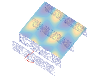
We will exploit the shallowness of OCFs in order to tackle the problem at hand with the aid of depth-averaged equations. With this aim, Reynolds-averaged Navier–Stokes equations (RANS) will be integrated along the bed-normal coordinate, by paying attention to preserving the dispersive terms arising from the momentum transport coupling between the longitudinal and transverse velocity profiles. In the depth-averaged procedure, such dispersive terms will appear in the form of integral factors. This trick is particularly suitable when applied to a flow field that, under undisturbed conditions, is composed by a primary longitudinal flow and a secondary recirculating current (see figure 1). The ultimate goal of the present approach is to perform a stability analysis of the secondary currents in order to discuss their role in triggering large-scale turbulence structures. This is usually referred to as a secondary stability analysis in hydrodynamic stability theory (e.g. Drazin & Reid Reference Drazin and Reid2004; Bertagni, Perona & Camporeale Reference Bertagni, Perona and Camporeale2018).

Figure 1. Three-dimensional view of the flow field.  $(a)$ The undisturbed secondary cells.
  $(b)$ Symmetry breaking of the secondary cells from the perturbative solution under the most unstable conditions (
 $\omega =0.006$;
  $\epsilon =0.005$;
  $L_x=4$;
  $L_z=2$ (
 $\beta ={\rm \pi}$);
  $F=0.7$;
  $d=0.01$, see § 3 for details). Colour shading refers to the perturbation of the flow field with troughs (lighter) and peaks (darker). Red arrows refer to the primary longitudinal flow
  ${\cal {F}}(y)$.
2.1. Framework
The OCFs can be described by RANS equations flanked by suitable boundary conditions, such as the kinematic and dynamic conditions at the free surface, and no slip and impermeability at the bed. We will adopt the bulk longitudinal velocity  $\hat {U}_0$, the channel depth
  $\hat {h}_0$, the corresponding hydrodynamic time scale
  $\hat {h}_0/\hat {U}_0$ and
  $\rho {\hat {U}}_0^2$ to non-dimensionalize velocities, lengths, times and pressure, respectively (
 $\rho$ is the water density). Body forces are non-dimensionalized by the module of the gravity acceleration. Henceforth, the hat symbol identifies dimensional quantities.
As reported in the sketch of figure 1, we consider the (dimensionless) reference frame  ${x}_i=(x,y,z)$, having axes parallel to the streamwise, bed-normal and spanwise directions, respectively. The corresponding Reynolds-averaged velocity term is
  $\boldsymbol {u}:=(u,v,w)$. Assuming high Reynolds numbers and hence negligible viscous stresses, the non-dimensional RANS equations read as
 $$\begin{gather} \frac{\partial{\boldsymbol{u}}}{\partial{t}}+\boldsymbol{u}\boldsymbol{\cdot}\boldsymbol{\nabla} \boldsymbol{u}+\boldsymbol{\nabla}{p} + \boldsymbol{\nabla} \boldsymbol{\cdot} \boldsymbol{\tau}-\frac{\boldsymbol{k}}{F^2}=0, \end{gather}$$
 $$\begin{gather}\boldsymbol{\nabla}\boldsymbol{\cdot}\boldsymbol{u}=0, \end{gather}$$
where  $F=\hat {U}_0/({g \hat {h}_0})^{1/2}$ is the Froude number, g is the gravity acceleration, p is pressure,
  $\boldsymbol {\tau }$ is the dimensionless Reynolds stress tensor,
  $\boldsymbol {k}=(\sin {\theta },-\cos {\theta },0)$ is the projection of the gravity unit-vector along the chosen coordinate system, with
  $\theta$ being the slope of the bed, with respect to a horizontal plane (see figure 1).
2.2. Secondary currents of Prandtl's second kind in OCF
Secondary currents are cellular structures with longitudinal vorticity (see figure 1 $a$) that appear in the time-averaged flow. In the present paper, we consider the case of a straight open channel in uniform flow conditions, whereby secondary flows are of Prandtl's second kind as they are the result of a combined effect between the three-dimensionality of the flow imposed by lateral boundaries and the anisotropy of turbulence (Nezu & Nakagawa Reference Nezu and Nakagawa1993). Secondary currents are clearly triggered in proximity to lateral boundaries where they occur in the form of ‘corner vortices’ and are characterized by intense lateral and vertical mean velocities. Their cellular structure then replicates along the lateral direction as a result of mass and momentum conservation, but their intensity fades out while moving towards the centre of the channel, so much so that they become difficult to detect experimentally (Zampiron, Cameron & Nikora Reference Zampiron, Cameron and Nikora2020). Nevertheless, Adrian & Marusic (Reference Adrian and Marusic2012) pointed out that, even for the case of very wide channels (i.e. channels whose width is much greater than their depth), secondary currents should be present, however weak, even in the mid-cross-section.
From a hydrodynamic instability point of view, a classical result indicates that, for a sufficiently shallow rectangular channel, the footprint of secondary currents on the spanwise profile of the streamwise (time-averaged) velocity can be interpreted as a turbulence-induced instability. The structure of such an instability in the  $(y,z)$ cross-section was obtained by Ikeda (Reference Ikeda1981) and Nezu & Nakagawa (Reference Nezu and Nakagawa1993) after a term-by-term order of magnitude analysis of the time-averaged vorticity budget equation. By imposing a balance between the production of vorticity due to turbulence anisotropy and the suppression of vorticity due to Reynolds shear stress, assuming that the difference in the Reynolds normal stresses is linearly
  $y$-distributed, and the bed shear stress is laterally periodically perturbed, Ikeda (Reference Ikeda1981) came to a solution for the velocity field imposed by secondary currents which, by employing the dimensionless parameters introduced in the present work, reads as
 \begin{equation} v_0={-}\omega\beta{{\cal{G}}(y)}\cos{(\beta z)},\quad w_0=\omega\frac{\textrm{d}{\cal{G}}(y)}{\textrm{d}y}\sin{(\beta z)}. \end{equation}
An approximated derivation of (2.3a,b) from (2.1), and a general solution for the distribution of the vertical velocity  ${\cal {G}}$ is detailed in Appendix A. The parameter
  $\omega$ is physically dependent on the Reynolds number and the channel aspect ratio (i.e. the ratio between channel width and depth), that accounts for circulation of the cell. The transverse wavenumber
  $\beta =2{\rm \pi} /L_z$ accounts for the lateral spacing (
 $L_z$) of secondary currents. According to Townsend (Reference Townsend1976), in the absence of longitudinal bed forms such as ridges, the dominant cell refers to the case
  $\beta ={\rm \pi}$, whereby the cell width and the depth are identical (
 $L_z/2=1$). A cross-stream view of the secondary current structure is shown in figure 1
 $(a)$.
In the results section, it will be shown that  $\omega$ is of paramount importance since it accounts for the intensity of secondary cells. In fact, by depth averaging (2.3a,b) and computing the circulation along a curve
  ${\cal {L}}$ lying on the plane
  $y-z$ and embracing a whole cell, we readily obtain that
 \begin{equation} \omega=\frac{1}{2{\rm \pi}}\left|\oint_{\cal{L}} (v_0,w_0)\boldsymbol{\cdot}\,\textrm{d}\kern0.06em {\boldsymbol x}\right|=\frac{\varOmega_x}{2{\rm \pi}},\quad\text{and}\quad\omega=\left|\frac{{\rm \pi}\langle{v_0}\rangle}{4 - {\rm \pi}^2}\right|_{z=0,\beta={\rm \pi}}, \end{equation}
where brackets indicate the depth-averaging operator. Thus  $\omega$ is proportional to the circulation of the velocity field around a curve embracing a whole cell. From the Stokes theorem, this can be interpreted as the value of the streamwise vorticity averaged over the surface covered by a cell (
 $\varOmega _x$) and hence a proxy for the intensity of secondary currents. It is noteworthy that the above result is independent of the shape of the primary velocity distribution
  $\cal {F}(y)$. Equation (2.4a,b) also shows that this value can be easily obtained by depth averaging the (non-dimensional) vertical velocity component
  $v_0$ from experimental data.
2.3. Depth-averaged equations
In order to derive the equations describing the dynamics of the problem at hand, we adopt the well-known shallow-water approximation (Tan Reference Tan1992), whereby  $\hat {h}_0$ is much smaller than the dominant horizontal length scales. Moreover, we assume that the longitudinal velocity components
  $u$ can be described by the factorization
  $u=\cal {F}(y)U(x,z,t)$, whereas the lateral velocity component is decomposed into a component related to the secondary current, that is with zero depth averaging, plus a vertically uniform spanwise component, namely
  $w=w_0(y,z)+W(x,z,t)$. Therefore,
  $U$ and
  $W$ are the depth-averaged longitudinal and lateral velocities, respectively. Under these hypotheses and upon depth averaging, (2.1) reduces to
 $$\begin{gather} \frac{\partial{\boldsymbol{U}}}{\partial{t}}+{\boldsymbol{U}}\boldsymbol{\cdot}\boldsymbol{\nabla}_{ {\perp}}{{\boldsymbol{U}}}+\frac{\boldsymbol{\nabla}_{ {\perp}}{\zeta}}{F^2}-\frac{\boldsymbol{\nabla}_{ {\perp}} \boldsymbol{\cdot} ({h}{\boldsymbol{T}})}{h}-\frac{\boldsymbol{\tau}_b}{h}=0, \end{gather}$$
 $$\begin{gather}\frac{\partial h}{\partial t}+\boldsymbol{\nabla}_{ {\perp}} \boldsymbol{\cdot} (h\boldsymbol{U})=0, \end{gather}$$
where  ${\boldsymbol {U}}(x,z,t)=\{U,W\}$ is the depth-averaged Reynolds-averaged flow field,
  $\boldsymbol {\nabla }_{ \perp }=\{\partial _x,\partial _z\}$,
  $\zeta =h - x\sin {\theta }$ is the free surface elevation,
  $h(x,z,t)$ is the water depth,
  $\boldsymbol {\tau }_b$ is the bottom shear stress and
  ${\boldsymbol {T}}$ is a
  $(2\times 2)$ tensor resulting from the sum of the depth-averaged Reynolds stress tensor and the dispersive tensor arising from depth averaging;
  $\boldsymbol {\tau }_b$ and
  ${\boldsymbol {T}}$ can be modelled by means of the Chezy and Boussinesq formulations as
 $$\begin{gather} \boldsymbol{\tau}_b={-}c_f{\boldsymbol{U}}|\boldsymbol{U}|, \end{gather}$$
 $$\begin{gather}\boldsymbol{T}=\langle\nu_t(\boldsymbol{\nabla}_{{\perp}}{\boldsymbol{u}}_{{\perp}}+\boldsymbol{\nabla}_{{\perp}}{\boldsymbol{u}}_{{\perp}}^T)\rangle-\langle(\boldsymbol{u}_{{\perp}}-\boldsymbol{U})\otimes(\boldsymbol{u}_{{\perp}}-\boldsymbol{U})\rangle, \end{gather}$$
where  $c_f=\sin {\theta }/F^2$ is the friction factor, which depends on the relative bed roughness
  $d\boldsymbol{\cdot }{h}^{-1}$ and the Reynolds number
  $Re$,
$Re$,  ${\boldsymbol {u}}_{\perp }=\{u,w\}$,
  $\nu _t=\sqrt {c_{f}}hU{{\cal {N}}(y)}$ is the eddy viscosity, brackets refer to depth averaging and
  $\otimes$ refers to the dyadic product. The shape of function
  ${\cal {N}}(y)$ that defines the eddy viscosity
  $\nu _t$ will be derived in § 4. The first term on the right-hand side of (2.8) accounts for the depth averaging of the Reynolds stresses, while the second one produces the so-called dispersive terms that arise from departure of plug flow conditions.
Two remarks are in order. Firstly, the vector equation (2.5) states the momentum conservation along the longitudinal and transverse directions and it was derived assuming that the vertical momentum conservation reduces to the hydro-static balance  $p \sim {F}^{-2}(h - y)$. This condition is the hallmark of the shallow-water equations and it can be shown from a dimensional analysis of the momentum conservation along the vertical direction, that it is constrained to the condition that the channel aspect ratio is much larger than the Froude number. Equation (2.6) states mass continuity after the use of the kinematic condition at the free surface (namely
  $\partial _{t}{h}=w - u_{\perp } \boldsymbol {\cdot } \boldsymbol {\nabla }_{ \perp }h$). Secondly, depth averaging of the longitudinal velocity provides
  $\langle {\cal {F}}\rangle =1$ by construction while
  $\langle {w}_0\rangle \sim \langle {\textrm {d}\cal {G}}/{\textrm {d}y}\rangle \sim 0$, for
  $\beta \sim {\rm \pi}$. From the above remarks, we obtain that (2.8) reads as
 \begin{equation}
\boldsymbol{T}=\sqrt{c_{f}}\,U\left( \begin{array}{@{}cc@{}}
\dfrac{1-\cal{I}_4}{\sqrt{c_{f}}}U+2h{\cal{I}}_0\dfrac{\partial
U}{\partial x} & h{\cal{I}}_0\dfrac{\partial
U}{\partial y}+h{\cal{I}}_1\dfrac{\partial W}{\partial
x}-\dfrac{{\cal{I}}_2 \omega\sin (\beta
z)}{\sqrt{c_{f}}} \\ h{\cal{I}}_0\dfrac{\partial
U}{\partial y}+h{\cal{I}}_1\dfrac{\partial W}{\partial
x}-\dfrac{{\cal{I}}_2 \omega\sin (\beta
z)}{\sqrt{c_{f}}} & 2h{\cal{I}}_1\dfrac{\partial
W}{\partial z}+2h{\cal{I}}_3 \beta \omega \cos (\beta
z)-\dfrac{{\cal{I}}_5\omega^2}{U\sqrt{c_{f}}}\left[\sin{\left(\beta{z}\right)}\right]^2
\end{array} \right), \end{equation}
\begin{equation}
\boldsymbol{T}=\sqrt{c_{f}}\,U\left( \begin{array}{@{}cc@{}}
\dfrac{1-\cal{I}_4}{\sqrt{c_{f}}}U+2h{\cal{I}}_0\dfrac{\partial
U}{\partial x} & h{\cal{I}}_0\dfrac{\partial
U}{\partial y}+h{\cal{I}}_1\dfrac{\partial W}{\partial
x}-\dfrac{{\cal{I}}_2 \omega\sin (\beta
z)}{\sqrt{c_{f}}} \\ h{\cal{I}}_0\dfrac{\partial
U}{\partial y}+h{\cal{I}}_1\dfrac{\partial W}{\partial
x}-\dfrac{{\cal{I}}_2 \omega\sin (\beta
z)}{\sqrt{c_{f}}} & 2h{\cal{I}}_1\dfrac{\partial
W}{\partial z}+2h{\cal{I}}_3 \beta \omega \cos (\beta
z)-\dfrac{{\cal{I}}_5\omega^2}{U\sqrt{c_{f}}}\left[\sin{\left(\beta{z}\right)}\right]^2
\end{array} \right), \end{equation}
with
 \begin{align}
{\cal{I}}_0=\langle{\cal{F}}{\cal{N}}\rangle,\enspace
{\cal{I}}_1=\langle{\cal{N}}\rangle,\enspace
{\cal{I}}_2=\langle{\cal{F}}{\cal{G}'}\rangle,\enspace
{\cal{I}}_3 = \langle{\cal{N}}{\cal{G}'}\rangle
\sim 0,\enspace
{\cal{I}}_4=\langle{\cal{F}}^2\rangle,\enspace
{\cal{I}}_5=\langle{\cal{G}'}^2\rangle,
\end{align}
\begin{align}
{\cal{I}}_0=\langle{\cal{F}}{\cal{N}}\rangle,\enspace
{\cal{I}}_1=\langle{\cal{N}}\rangle,\enspace
{\cal{I}}_2=\langle{\cal{F}}{\cal{G}'}\rangle,\enspace
{\cal{I}}_3 = \langle{\cal{N}}{\cal{G}'}\rangle
\sim 0,\enspace
{\cal{I}}_4=\langle{\cal{F}}^2\rangle,\enspace
{\cal{I}}_5=\langle{\cal{G}'}^2\rangle,
\end{align}
whose exact formulation was obtained upon making a specific choice for  $\cal {F}$ (see § 4) and is reported in Appendix B.
At the base state ( $\partial _t=\partial _x=0$), after combining (2.3a,b) with (2.5)–(2.9), and recalling that
  $\omega \ll {1}$, it appears that the effect of the secondary currents on the streamwise and spanwise momentum conservation is a
  $z$-dependent modulation to the longitudinal velocity and depth, respectively,
  $u_0=\cal {F}(y)U_0(z)$, and
  $h_0(z)$ with
 $$\begin{gather} U_0=1-\omega\varPhi_{1}\cos{(\beta z)}-\omega^{2}\left[\tfrac{1}{4}{\varPhi_{1}^2}-\varPhi_{2}\cos{(2\beta{z})}\right]+{O}(\omega^4), \end{gather}$$
 $$\begin{gather}h_0=1+\tfrac{1}{2}\omega^2F^2{\cal{I}}_5\cos{(2\beta{z})}+{O}(\omega^4), \end{gather}$$
where
 \begin{align} \varPhi_{1} =
\frac{\beta{\cal{I}}_2}{\sqrt{c_{f}} \left(2
\sqrt{c_{f}}+\beta ^2 {\cal{I}}_{0}\right)},\quad
\varPhi_{2} = \frac{F^{2}{\cal{I}}_{5} (c_{f} -
c_{f,h}) \left(2 \sqrt{c_{f}} + \beta ^2
{\cal{I}}_{0}\right)^2 + 3\beta ^2
{\cal{I}}_{2}^2}{4\sqrt{c_{f}}\left(2 \sqrt{c_{f}} -
\beta ^2 {\cal{I}}_{0}\right)^2 \left(\sqrt{c_{f}} + 2
\beta ^2 {\cal{I}}_{0}\right)},
\end{align}
\begin{align} \varPhi_{1} =
\frac{\beta{\cal{I}}_2}{\sqrt{c_{f}} \left(2
\sqrt{c_{f}}+\beta ^2 {\cal{I}}_{0}\right)},\quad
\varPhi_{2} = \frac{F^{2}{\cal{I}}_{5} (c_{f} -
c_{f,h}) \left(2 \sqrt{c_{f}} + \beta ^2
{\cal{I}}_{0}\right)^2 + 3\beta ^2
{\cal{I}}_{2}^2}{4\sqrt{c_{f}}\left(2 \sqrt{c_{f}} -
\beta ^2 {\cal{I}}_{0}\right)^2 \left(\sqrt{c_{f}} + 2
\beta ^2 {\cal{I}}_{0}\right)},
\end{align}
with  $c_{f,h}={\partial {c_f}}/{\partial {h}}|_{h=1}$. Equation (2.11) is crucial for the following analysis since it will be shown that such a transverse modulation, combined with the free surface response, induces an instability of the inflectional type to the secondary currents. It is straightforward to show that the terms of order
  ${O}({\omega ^3})$ are zero in the above expansions. It is also worth noticing that (2.11) is reminiscent of the spanwise modulation derived by Waleffe (Reference Waleffe1995), for the case of streamwise rolls superimposed on a laminar Couette flow. In the following analysis we will neglect terms of order
  $\omega ^2$ or higher, since they complicate the algebraic treatment without any numerically relevant effect (see Appendix E).
3. Stability analysis
3.1. Perturbative solution
In order to account for large-scale longitudinal meandering of the secondary cell axis, let us consider a time-dependent normal-mode perturbation, by adopting the following putative solution to (2.5)–(2.6):
 \begin{equation} \{U,W,h\}=\{U_0,0,h_0\}+\epsilon\{U_1(z),W_1(z),h_1(z)\}\exp({{\textrm{i}}\alpha{x}+\lambda t})+\textrm{c.c.}, \end{equation}
where the base state  $U_0$ and
  $h_0$ are provided by (2.11) and (2.12) truncated at order
  $\omega$,
  $\epsilon$ is a small perturbative parameter,
  $\alpha$ is the longitudinal wavenumber of the perturbation,
  $\lambda$ is its growth rate and
  $\textrm {c.c.}$ refers to complex conjugation.
It is important to remark that under non-uniform and unsteady conditions the friction factor depends on the local value of the depth, through the ratio  $d \boldsymbol{\cdot} {h}^{-1}(x,z,t)$. This aspect is accounted for through a Taylor expansion as follows:
 \begin{equation} c_f(h)\sim\left.{c}_{f}\right|_{h=1}+\left.\frac{\partial{c_f}}{\partial{h}}\right|_{h=1}(h-1)=c_{f0}+\epsilon\left.\frac{\partial{c_f}}{\partial{h}}\right|_{h=1}h_1 \textrm{e}^{\textrm{i}\alpha{x}+\lambda{t}}+\textrm{c.c.}, \end{equation}
where  $c_{f0}={c}_{f}|_{h=1}$ is the friction factor computed for the unperturbed flow. After substituting the above ansatz in (2.5)–(2.6) and taking into account (2.7)–(2.13a,b), at the order
  $\epsilon$ we obtain the eigenvalue problem
 \begin{equation} u_*(\boldsymbol{A}+\omega\boldsymbol{B})\boldsymbol{q}={\lambda}\boldsymbol{q}, \end{equation}
where  $\boldsymbol {q}=\{U_1,W_1,h_1\}^T$, while
  $u_*$:=
 $\sqrt {c_{f0}}$ is the dimensionless friction velocity, and
 \begin{gather} \boldsymbol{A}=\left( \begin{array}{@{}ccc@{}} {\cal{I}}_0{\cal{D}}^2 - \sigma_0 & \textrm{i}\,{\cal{I}}_1\alpha{\cal{D}} & \sigma_1 \\ \textrm{i}\cal{I}_0\alpha\cal{D} & 2\cal{I}_1\cal{D}^2-\sigma_4 & -\dfrac{\cal{D}}{u_*F^2}\\ -\dfrac{\textrm{i}\alpha}{u_*} & -\dfrac{\cal{D}}{u_*} & -\dfrac{\textrm{i}\alpha}{u_*} \end{array} \right), \end{gather}
 \begin{gather} \boldsymbol{B}=\left( \begin{array}{@{}ccc@{}} \sigma_2\cal{C}+\sigma_9 \cal{S}\cal{D} -\dfrac{\textrm{i}\sigma_6}{\alpha }\cal{C}\cal{D}^2 & -\dfrac{\textrm{i}\alpha\beta\sigma_8}{2}\cal{S} -\dfrac{ \sigma_7\beta}{u_*}\cal{S} + \dfrac{\textrm{i}\alpha\sigma_8}{2} \cal{C}\cal{D} & \sigma_3\cal{C} + \sigma_9 \cal{S}\cal{D} \\ \sigma_5 \cal{S} + \sigma_6\cal{C}\cal{D} & \sigma_7 \sigma_4 \cal{C} + \sigma_8(\cal{C}\cal{D} - \beta\cal{S})\cal{D} & \textrm{i}\,\alpha \sigma _9 \cal{S}\\ 0 & 0 & \dfrac{\textrm{i}\,\alpha\sigma_7}{u_*}\cal{C} \end{array} \right). \end{gather}
 In these matrices  $\cal {D}^n=\text {d}^n/\text {d}z^n$,
  $\cal {C}=\cal {C}(z)=\cos {(\beta {z})}$,
  $\cal {S}=\cal {S}(z)=\sin {(\beta {z})}$, while the coefficients
  $\sigma _i$ are reported in Appendix C. The presence of the functions
  $\cal {C}$ and
  $\cal {S}$ in
  $\boldsymbol {B}$ precludes an analytical solution of (3.3), unless
  $\omega =0$.
3.2. Spectral solution of the eigenvalue problem
We firstly consider the mapping  $z \rightarrow {\xi }=\beta {z}$, so that the operators
  $\boldsymbol {A}$ and
  $\boldsymbol {B}$ become periodic in the interval
  $\xi =[0,2{\rm \pi} ]$. The differential eigenvalue problem (3.3) may be solved by a Fourier Galerkin spectral method (see e.g. Canuto et al. Reference Canuto, Hussaini, Quarteroni and Zang2006). Accordingly, a modal representation of the approximate solution with trigonometric polynomials is adopted
 \begin{equation} \boldsymbol{q}=\sum_{k={-}N/2}^{k=N/2}\hat{\boldsymbol{q}}_k \textrm{e}^{{\text{i}}k\xi}, \end{equation}
where the cutoff parameter  $N$ is an even arbitrarily large integer.
A weak formulation of the problem is obtained by selecting a set of test functions  $\boldsymbol {\psi }_{l,n}$ that determine the weights of the residual
 \begin{equation} \int_0^{2{\rm \pi}}[u_*(\boldsymbol{A}+\omega\boldsymbol{B})-\lambda\boldsymbol{I}]\boldsymbol{q}{\boldsymbol{\psi}}_{l,n}\,\textrm{d}\xi=0,\quad (n={-}N/2,\ldots,N/2;\quad l=1,\ldots,6). \end{equation}
A natural choice of the test functions is  $\boldsymbol {\psi }_{l,n}=(2{\rm \pi} )^{-1}\boldsymbol {v}_l{e}^{-{\text {i}}n\xi }$, where
  $\boldsymbol {v}_l$ is any vector of the canonical basis in
  $\mathbb {C}^3$ (i.e. one component is equal to 1 or
  $\text {i}$, all the others
  $0$).
$0$).
In order to reduce (3.7) to an algebraic eigenvalue problem, let us first observe that, by expressing  $\cos {\xi }$ and
  $\sin {\xi }$ in terms of exponentials
  $\textrm {e}^{\pm {\text {i}}\xi }$, one can decompose the matrix
  $\boldsymbol {B}$ in (3.7) as
 \begin{equation} \boldsymbol{B}=\textrm{e}^{-\text{i}\xi}\boldsymbol{B}_{{-}1}+\textrm{e}^{\text{i}\xi}\boldsymbol{B}_{1}=\sum_{j={\pm}{1}}\textrm{e}^{\text{i}j\xi}\boldsymbol{B}_j, \end{equation}
where  $\boldsymbol {B}_j$ are the matrices with constant coefficients with respect to
  $\xi$, similarly to the matrix
  $\boldsymbol {A}$ in (3.4). Hence,
 \begin{align} [u_*(\boldsymbol{A}+\omega\boldsymbol{B}) - \lambda\boldsymbol{I}]\boldsymbol{q}&=\sum_{k={-}N/2}^{N/2}\left[u_*\left(\boldsymbol{A}+ \omega\sum_{j={\pm}{1}} \textrm{e}^{\text{i}j\xi}\boldsymbol{B}_j\right)-\lambda\boldsymbol{I}\right] \textrm{e}^{\text{i}k\xi}\hat{\boldsymbol{q}}_k\nonumber\\ &=\sum_{k={-}N/2}^{N/2}\left[u_*\left(\hat{\boldsymbol{A}}_k+ \omega\sum_{j={\pm}{1}} \textrm{e}^{\text{i}j\xi}\hat{\boldsymbol{B}}_{j,k}\right)-\lambda\boldsymbol{I}\right] \textrm{e}^{\text{i}k\xi}\hat{\boldsymbol{q}}_k\nonumber\\ &=\sum_{k={-}N/2}^{N/2}\left[u_*\left(\hat{\boldsymbol{A}}_k\hat{\boldsymbol{q}}_k \textrm{e}^{\text{i}k\xi}+ \omega\sum_{j={\pm}{1}}\hat{\boldsymbol{B}}_{j,k}\hat{\boldsymbol{q}}_k \textrm{e}^{\text{i}(k+j)\xi} \right)-\lambda\hat{\boldsymbol{q}}_k \textrm{e}^{\text{i}k\xi}\right], \end{align}
where the matrices  $\hat {\boldsymbol {A}}_k$,
  $\hat {\boldsymbol {B}}_{j,k}$ are obtained from
  ${\boldsymbol {A}}$,
  ${\boldsymbol {B}}_{j}$ by replacing the derivative operator
  $\cal {D}=\text {d}/\text {d}\xi$ by
  $\text {i}k$ (Fourier differentiation). The entries of these matrices are reported in Appendix D.
After substituting (3.9) in (3.7), one easily obtains the algebraic eigenvalue problem of order  $3(N+1)$
 \begin{equation} u_*\left(\hat{\boldsymbol{A}}_{n}\hat{\boldsymbol{q}}_n+\omega\sum_{j={\pm}{1}}\hat{\boldsymbol{B}}_{j,n-j}\hat{\boldsymbol{q}}_{n-j}\right)={\lambda}\hat{\boldsymbol{q}}_n, \quad (n={-}N/2,\ldots,N/2). \end{equation}
Note that the matrix of order  $3(N + 1)$ corresponding to the left-hand side is block tridiagonal, with diagonal blocks given by
  $u_*\hat {\boldsymbol {A}}_{n}$ and off-diagonal blocks given by
  $u_*\omega \hat {\boldsymbol {B}}_{1,n-1}$ (left), and
  $u_*\omega \hat {\boldsymbol {B}}_{-1,n+1}$ (right). A ready-to-use set of Matlab scripts for the solution of (3.10) can be found in the supplementary material available at https://doi.org/10.1017/jfm.2021.769.
4. Results
We consider the simplest and most common choice for the velocity distribution, namely the well-known log law for the mean velocity distribution
 \begin{equation} \cal{F}=\frac{\sqrt{c_{f}}}{\kappa}\log{\frac{y}{y_0}}, \end{equation}
where  $\kappa$ is the von Kármán constant and
  $y_0$ is the roughness length. By inserting (4.1) in the streamwise component of (2.1), and accounting for steady uniform flow conditions, we obtain
 \begin{equation} y\frac{\textrm{d}\kern0.7pt\cal{N}}{\textrm{d}y}+\kappa{y^2}-\cal{N}=0. \end{equation}
By imposing zero turbulence on the free surface,  $\cal {N}(1)=0$, the classical parabolic solution for the eddy viscosity can be recovered, namely,
  $\cal {N}=\kappa y(1-y)$. In addition,
  $\langle {{\cal {F}}}\rangle =1$ by construction, so from (4.1) the friction factor
  $c_f$ can be computed as
 \begin{equation} \sqrt{c_f}=\frac{\kappa}{\dfrac{y_0}{h}-1-\log{\dfrac{y_0}{h}}}. \end{equation}
 In hydraulically rough-bed conditions (very relevant in fluvial environments), the roughness length is usually set proportional to the mean (dimensionless) diameter of the equivalent sediment grain  $d$ (or other features of the grain distribution). By setting the equivalence between (4.3) and Strickler's formula for a hydraulically rough wall,
  $\sqrt {c_{f0}}=\sqrt {g}d^{1/6}/21$, we obtain
  $y_0\sim {d/15}$. Therefore, in this case the friction factor is independent of the Reynolds number.
In summary, the parameter space of the present problem is reduced to:  $\alpha$,
  $\beta$,
  $F$,
$F$,  $d$ and
  $\omega$. The case of hydraulically smooth wall will not be analysed since it is not relevant to fluvial applications and it has been poorly investigated experimentally. Yet, we have verified that it performs, qualitatively, as in the rough wall case.
It is straightforward to show that the case without secondary currents ( $\omega =0$) is invariably stable. This case is in fact described by the eigenvalues of the operator
  $\boldsymbol {A}$, which admits eigenfunctions proportional to
  $\exp {(\text {i}k\beta {z})}$ where
  $k$ is integer. The problem is therefore reduced to the solution of
  $k$ cubic equations whose roots have all negative real parts, for any
  $k$ (see black circles in figure 2). This result confirms the robustness of the canonical shallow-water equations to harmonic perturbations and suggests that there exists a threshold value
  $\omega _c$ of
  $\omega$ that is necessary to trigger the instability of secondary currents (see white squares in figure 2
 $b$). Through a sensitivity analysis (not show here) we observed that
  $\omega _c$ ranges in a thin interval
  $[1.4\text {--}3.2] \times {10}^{-3}$.

Figure 2.  $(a)$ Eigenvalue spectra.
  $(b)$ Zoom in the neighbourhood of the imaginary axis. Closed symbols,
  $\omega =0$; open symbols,
  $\omega =0.02$;
  $\beta ={\rm \pi}$;
  $d=0.01$;
  $F=0.7$;
  $\alpha ={\rm \pi} /2$;
  $N=350$. The arrow indicates the (only) unstable mode.
In the case  $\omega > 0$, the problem needs to be solved by using the spectral method illustrated in § 3.2. A reliability test for the developed algorithm has validated the exponential convergence in the accuracy of the method vs the cutoff
  $N$, showing that 20–30 modes are sufficient to reach machine precision. The relative error has been assessed with respect to the value computed with maximum precision (
 $N=70$ in figure 3). Figure 3 identifies two modes of instability that are detected by the present approach. The first one is related to the occurrence of roll waves (panel
  $a$), which are foreseen at
  $F>1.5$, in the limit of infinite lateral spacing of the perturbation (
 $L_z \rightarrow \infty$). Such cylindrical perturbations of the free surface are typical of very steep beds and are unaffected by secondary currents. The shape of the unstable domain of the roll waves is reproduced in agreement with other previous theories (Camporeale, Canuto & Ridolfi Reference Camporeale, Canuto and Ridolfi2012; Caruso et al. Reference Caruso, Vesipa, Camporeale, Ridolfi and Schmid2016). Furthermore, the present theory provides an improvement with respect to the classical shallow-water theory based on the linearized Saint-Venant equations (Whitham Reference Whitham1974), where roll-wave instability is expected at
  $F > 2$, for any longitudinal wavelength. In particular, the reduction of the critical Froude number
  $F_c$ to the value
  $1.5$ is due to Taylor's expansion of the friction factor
  $c_f$ (3.2), and provides a result that is consistent with previous linearized approaches. Following a criterion of instability introduced by Dressler (Reference Dressler1949), the critical Froude number reads
 \begin{equation} F_c=[\varPsi^2-(2\varPsi-1)\cal{I}_4]^{{-}1/2}, \end{equation}
where  $\varPsi =(3 - c_{f,h}/c_{f0})/2$ (see also Arai, Huebl & Kaitna (Reference Arai, Huebl and Kaitna2013) for a modern treatment). The above equation provides the classical result
  $F_c=2$ when
  $c_f=c_{f0}$,
  $\cal {I}_4=1$ and the term
  $[\partial {c_f}/\partial {h}]_{h=1}\equiv {c}_{f,h}$ is set to zero. On the contrary, when
  $c_{f,h} \neq {0}$, (4.4) gives that
  $F_c$ decreases from 1.7 to 1.63 for
  $d=[0.001\text {--}0.01]$, that is in agreement with our results.

Figure 3. Contour plot of the growth rate Re $[\lambda _1]$ in the
  $\alpha - F$ plane (
 $d=0.01$ ).
  $(a)$ Roll-wave mode for
  $\beta \sim {0}$ (
 $L_z \rightarrow \infty$) and
  $\omega =0$.
  $(b)$ Sinuous mode for
  $\beta ={\rm \pi}$ (
 $L_z=2$) and
  $\omega =0.041$.
The second mode of instability (panel  $b$) is the main focus of the present paper. It is detected when the spacing between counter-rotating secondary cells is nearly equal to the depth (
 $L_z=2$) and it is characterized by a symmetry breaking of the secondary currents induced by the development of waves that are about four depths long in the streamwise direction (
 $L_x=4$, see also figure 1
 $b$).
$b$).
The value of the least stable eigenvalue  $\lambda \equiv \lambda _{1}$, as obtained by the spectral method described in § 3.2, is reported vs the longitudinal wavelength
  $L_x=2{\rm \pi} \alpha ^{-1}$ for various
  $\omega$ values (figure 4
 $a$). It is evident that the growth rate always displays a maximum at a particular longitudinal wavelength
  $L_x=L_x^{max}$ and then decays for longer and shorter wavelengths. This means that the linear stability analysis is able to select a longitudinal wavelength, corresponding to the least stable mode, and the problem is well posed for larger and smaller length scales.

Figure 4. Growth rate vs the longitudinal wavelength for  $(a)$ different values of
  $\omega =[0.006\text {--}0.062]$ and
  $(F,d,L_z)=(0.7, 0.01, 2)$;
  $(b)$ different values of
  $L_z=[1.67\text {--}2.5]$ and
  $(F,d,\omega )=(0.7,0.01,0.04)$. The shaded areas mark the range of variability of
  $L_x^{max}$.
The selected wavelength  $L_x^{max}$ assumes almost constant values of approximately 3.5–4 times the depth, when the lateral spacing between cells is set to the experimentally observed value
  $L_z={2{\rm \pi} }/{\beta }=2$ (i.e. purely circular cells). These values of
  $L_x^{max}$ are well within the range of those reported for LSM wavelengths estimated in the outer layer of rough- and smooth-bed OCFs by Cameron et al. (Reference Cameron, Nikora and Stewart2017) and Peruzzi et al. (Reference Peruzzi, Poggi, Ridolfi and Manes2020) (note that in both papers the wavelength of the LSMs increases with increasing wall distance, from 2 to 6 times the depth). This suggest that LSM spectral peaks could be partly caused by an instability of secondary currents that is reminiscent of the sinuous-mode streak instability reported by CH for other wall flows and considered as the trigger of the outer-layer cycle (Park et al. Reference Park, Hwang and Cossu2011; Cossu & Hwang Reference Cossu and Hwang2017). We also notice that this result is quite robust to the choice of the free parameters. In particular, if the lateral spacing
  $L_z$ is allowed to vary over a broader range (
 $L_z=[1.5\text {--}2.5]$, see figure 4
 $b$), the selected wavelength
  $L^{max}_x$ remains locked between 3 and 4.5.
We remark that the analysis of the spectrum reveals that the present approach has a limit of validity that is identified by an upper bound on the parameter  $\omega$, henceforth referred to as
  $\omega _u$, above which the problem (3.3) exhibits a set of eigenvalues with positive real parts. These eigenvalues are not associated with any physical instability mode. Yet, it is worth noticing that such shortcomings are not an issue since they have effects when
  $\omega$ is very high, corresponding to non-physical values of the secondary current magnitude. The threshold value
  $\omega _u$ beyond which our theory is no longer valid can be fairly easily estimated as follows.
Consider the matrices  $\hat {\boldsymbol {A}}_k$ and
  $\hat {\boldsymbol {B}}_{\pm {1},k}$ introduced in § 3.2, which appear in the eigenvalue problem (3.10); neglecting the lower-order terms with respect to the wavenumber
  $k$, one obtains diagonal matrices with non-zero entries proportional to
  $k^2$, by which an eigenvalue problem similar to (3.10) can be defined. Solving it amounts to computing the eigenvalues of two tridiagonal matrices, whose non-zero entries in the
  $n$th row (
 $-N/2\leq n\leq N/2$) are given by
 \begin{equation} \omega b (n-1)^2, \quad an^2, \quad \omega b (n+1)^2, \end{equation}
for  $a=-{\cal {I}}_0\beta ^2$,
  $b={{\cal {I}}_0{\cal {\varPhi }}_1 \beta ^2}/{2}$ or
  $a=-2{\cal {I}}_1\beta ^2$,
  $b={\cal {I}}_1{\cal {\varPhi }}_1 \beta ^2$, where
  ${\cal \varPhi }_1$ is defined by (2.13a,b). Then, Gershgorin's circle theorem (Golub & Van Loan Reference Golub and Van Loan1996) guarantees that all such eigenvalues have non-positive real parts provided
  $\omega \leq {a}/{2b}=-{\cal {\varPhi }}_1^{-1}$; furthermore, clear numerical evidence indicates that positive eigenvalues appear as soon as
  $\omega$ exceeds this threshold. This analysis suggests that the threshold
  $\omega _u$ for the original eigenvalue problem (3.10) should satisfy
 \begin{equation} \omega_u\sim{-}{\cal{\varPhi}}_1^{{-}1}. \end{equation}
Notice that the above relation depends on the parameters  $d$ and
  $\beta$ only. Remarkably, a comparison of the right-hand side of (4.6) with the value of
  $\omega _u$ obtained from the numerical solution yields a discrepancy of less than 1
 $\%$, that is completely acceptable for practical purposes. More importantly, when considering the possible range of variation of
  $\beta$ and
  $d$, it turns out that
  $\omega _u$ is of order
  $10^{-1}$ or larger. Upon analysis of the results presented by e.g. Blanckaert, Duarte & Schleiss (Reference Blanckaert, Duarte and Schleiss2010), such values of
  $\omega _u$ seem significantly higher than those expected in OCFs over rough beds.
4.1. Inflectional and streak instabilities
The previous results open some questions on the cause–effect connection between the shape of secondary cells and the observed unstable modes. Lord Rayleigh's criterion states that the necessary condition for the instability of a parallel (inviscid) flow is that the basic velocity profile displays an inflection point. Fjørtoft's criterion also adds that the absolute vorticity is maximum at the inflection point (Schmid & Henningson Reference Schmid and Henningson2001). Due to the presence of inflection points in the transverse profile of the longitudinal flow and  $U_0(z)$ satisfying both conditions – see (2.11) – it is worth exploring to what extent the nature of the detected instability has an inflectional nature for example of the Kelvin–Helmholtz (KH) kind. In this context, mixing layers satisfy inflectional criteria and trigger KH-instabilities with a temporal frequency
  $f=a(U_M + U_m)/2 \theta$ (Ho et al. Reference Ho, Zohar, Foss and Buell1991), where
  $U_M$ and
  $U_m$ are the maximum and the minimum of the velocity profile, respectively, while
  $\theta$ is the momentum thickness
 \begin{equation} \theta=\frac{1}{4}\int_{z^-}^{z^+} \left[1-\left(\frac{2U_0-U_M-U_m}{U_M-U_m}\right)^2\right]\,\textrm{d}z, \end{equation}
with  $z^-$ and
  $z^+$ setting the boundaries of the profile. The coefficient
  $a$ is equal to 0.032 in the case of a hyperbolic–tangent velocity profile. Inflectional stability was also studied in the context of jets and vegetated canopies (Finnigan, Shaw & Patton Reference Finnigan, Shaw and Patton2009; Raupach & Shaw Reference Raupach and Shaw2009). More recently, by means of long-duration experiments using stereoscopic particle image velocimetry, Zampiron et al. (Reference Zampiron, Cameron and Nikora2020) experimentally observed a linear relation between the longitudinal wavelength of the secondary current instability and the vorticity thickness, i.e.
  $L_x \sim {b}\delta _{\omega }$, where
 \begin{equation} \delta_{\omega}=\frac{U_M-U_m}{\max\left|\dfrac{\textrm{d}U_0}{\textrm{d}z}\right|}. \end{equation}
The proportionality constant  $b$ was found to be equal to 9 by Zampiron et al. (Reference Zampiron, Cameron and Nikora2020) while a value of
  $15$ was obtained by Finnigan et al. (Reference Finnigan, Shaw and Patton2009) for canopy mixing layers and approximately
  $4$ by Dimotakis & Brown (Reference Dimotakis and Brown1976) for canonical mixing layers. It is important to notice that, in the experiments carried out by Zampiron et al. (Reference Zampiron, Cameron and Nikora2020) (most relevant for the present paper), secondary currents were amplified by placing longitudinal ridges on the channel bed and hence did not evolve naturally on a flat rigid bottom as in canonical uniform OCFs.
Because of the periodic nature of  $U_0(z)$, the flow field under consideration is subjected to a sequence of inflectional profiles, so it is convenient to set
  $z^{\pm }=\pm {{\rm \pi} /\beta }$. In this way, from (4.7) and (4.8) we obtain, respectively,
 \begin{equation} \theta=\frac{\rm \pi}{4\beta},\quad \delta_{\omega}=\frac{2}{\beta}. \end{equation}
 Figures 5 $(a)$ and 5
 $(b)$ report the instability frequency and the selected wavelengths vs
  $(U_M + U_m)/2 \theta$ and vorticity thickness, respectively, by spanning the whole range of (
 $F$,
$F$,  $\omega$,
  $L_z$) values investigated herein. We see that the present problem develops a temporal frequency
  $f\equiv {{\text {Im}}(\lambda _1)}$ that is in fact linearly related to the ratio between the mean velocity and the momentum thickness and the best fit is
  $f=0.07(U_M + U_m)/2 \theta$ (dashed line in figure 5
 $a$). Similarly, when the same data are reported in the
  $\delta _{\omega }-L_x$ plane (figure 5
 $b$), a linear relation between the selected wavelength and the vorticity thickness is also confirmed, with a proportionality constant of approximately 6, which is between the values reported by the case of mixing layers and the experiments by Zampiron et al. (Reference Zampiron, Cameron and Nikora2020).

Figure 5. Inflectional instability.  $(a)$ Relation between the temporal frequency of the least stable wave and the momentum thickness. The KH-instability in hyperbolic tangent profile (solid line); our results (dots);
  $f=0.07(U_M + U_m)/2 \theta$ (dashed line).
  $(b)$ Relation between the selected wavelength and the vorticity thickness. The dashed line refers to best fit of the dots (
 $F=[0.2\text {--}0.8]$;
  $\omega =[0.005\text {--}0.04]$;
  $L_z=[1.7\text {--}2.5]$).
The linear relations depicted in figure 5 suggest that the detected sinuous instability might be of an inflectional nature. Indeed, if the spanwise transport of the longitudinal momentum due to lateral gradients  $W\partial {U}/\partial {z}$ is inhibited – i.e. the second term of the entry
  $B_{12}$ in (3.5) is removed – then the mathematical problem becomes unconditionally stable. However, as will be pointed out in the subsequent discussion, the inflectional point alone is not a sufficient condition to trigger such an instability, because the presence of a free surface dynamically responding to perturbations is another key requirement.
Another fundamental instability that our work needs to be put into context with is the so-called streak instability, which is strictly linked with the well-known near-wall cycle and self-sustained process cycle investigated by Waleffe (Reference Waleffe1995, Reference Waleffe1997) in the case of laminar flows. Following the success of Waleffe's works, other authors have considered large-scale optimal streaks, and performed secondary stability analyses in turbulent closed-channel flows, by focusing on the outer layer (Park et al. Reference Park, Hwang and Cossu2011) or on the log layer (Alizard Reference Alizard2015). The use of solution (2.3a,b) as the starting point of a stability analysis and its connection to turbulence anisotropy sets further similarities with the vortex–wave interaction theory (Hall & Smith Reference Hall and Smith1988, Reference Hall and Smith1991; Waleffe Reference Waleffe2010; Hall Reference Hall2018), where long-wavelength coherent structures support the coexistence of rolls, streaks and waves. Resemblances of our results with those findings are encouraging, and might suggest framing the present instability in the context of the streak secondary instability. However, the depth-averaged approach herein adopted hides a close connection with the three-dimensional framework of the mentioned works.
As explained in the subsequent discussion, the key role of the free surface in setting the difference with respect to both streak instabilities (as performed by CH and Alizard Reference Alizard2015) and the KH instability will be commented on, suggesting that the right interpretation might be in between.
5. Discussion
In order to put the results obtained herein for OCFs within the wider context of wall flows, analogies and differences between the present work and those by CH are now identified and discussed.
Firstly, it is important to point out that, with respect to the CH approach, the proposed procedure does not require a transient growth analysis. The fact that OCFs develop steady secondary flow structures relieves the mathematical methodology from adopting non-normal analyses to identify optimal perturbations as the seedling of instabilities and permits us to keep the whole work within the remit of canonical linear stability analysis. In this context it is instructive to compare the present base state and the outcomes of the non-normal analyses previously developed by CH. In Hwang & Cossu (Reference Hwang and Cossu2010), the optimal transient perturbation of the flow field was generated by a body force artificially added to the linearized governing equations for closed-channel flows. This optimal body force is distributed within the flow domain in the form of counter-rotating cells with an aspect ratio close to one (see arrays in figure 6 $a$). In the original scaling adopted for closed channels, where
  $\delta$ is taken as the half-distance between plates, perfect circularity would correspond to
  $\hat {L}_z \sim {4}\delta$, while the exact value reported by the authors was
  $\hat {L}_z={3.5}\delta$. This suggests that, in the CH-approach, the external body force somewhat plays a similar role to the secondary currents (
 $v_0,w_0$) considered in (2.3a,b) in being the trigger of the instability. The streamwise velocity
  $u_0$, whose lateral structure is reported in (2.11) is akin to the outer longitudinal streaks detected in the transient analysis (contour lines in figure 6
 $b$). Note that secondary currents have a different topology with respect to the transient and body-force-induced velocity pattern reported in closed channels by CH (see figure 6). In CH, lines of constant longitudinal velocity are closed and anti-symmetrical with respect to the horizontal mid-plane. In our study, the same lines are bounded by the free surface. It is also important to recall that, in Hwang & Cossu (Reference Hwang and Cossu2010), the longitudinal streaks, which correspond to optimal perturbations, although being detected at vanishing values of the temporal frequency and longitudinal wavenumber, are a transient response of the system, while the secondary currents are features of the time-averaged flow.

Figure 6.  $(a)$ Cross-stream view of the optimal forcing (arrows) and the corresponding response in the streamwise velocity (contours) from the transient growth analysis in closed-channel flows (adapted from Hwang & Cossu Reference Hwang and Cossu2010).
  $(b)$ Cross-stream view of the secondary currents (arrows) described by (2.3a,b) and the corresponding response in the streamwise velocity (contours). In both panels solid contours refer to positive values, negative contours to negative values and the quantity
  $\delta$ refers to the channel depth.
Both the present stability analysis and the works by CH detect scales of motion comparable in size to LSMs, by resolving the response of the systems to the injection of an organized cellular structure (i.e. the optimal perturbation in the former, secondary currents in the latter). In both cases, the response of the system was identified to be sensitive to the intensity of the organized structure. In particular, de Giovanetti, Sung & Hwang (Reference de Giovanetti, Sung and Hwang2017) defined a measure of the streak amplitude  $A_s^+$, which is related to the control parameter
  $\omega$ as
 \begin{equation} A_s^+{=}\frac{\left|{\cal{\varPhi}}_1\right|}{u_*}\omega, \end{equation}
with  ${\cal {\varPhi }}_1$ defined by (2.13a,b). The same authors realized that the premultiplied spectral intensity of wall-normal velocity in the core of the flow for
  $L_x=3.57\delta$ abruptly increases when
  $A_s^+>4$. From (5.1) this threshold corresponds to
  $\omega =0.012$ when
  $d=0.001$. We detected that the critical values
  $\omega _c$ for the occurrence of the linear instability are of order
  $10^{-3}$, which suggests that OCFs are usually more unstable to LSMs than closed-channel flows. Incidentally, we notice that coupling equations (4.6) and (5.1), with
  $\omega =\omega _u$, it is easy to show that
  $A_{s,u}^+={c_{f0}^{-1/2}}$. We recall that the latter term depends on the wall roughness only, and it is usually larger than
  $10$. This means that the present theory is valid as long as
  $A_s^+\lesssim 10$.
It remains to explain the reason why a linear stability analysis of depth-averaged equations is sufficient to detect instabilities at wavelengths comparable to those of LSMs for OCFs, in place of the sophisticated nonlinear simulations adopted in closed channels. To this end, it is interesting to observe that, if the stability analysis is replicated under the rigid lid approximation, that is by artificially eliminating the dynamic character of the free surface (i.e. by forcing  $h_1=0$), then the problem turns to be unconditionally stable, as is evident in figure 7
 $(a)$. Therefore, the free surface plays a crucial role in triggering the linear instability, an aspect that is precluded in closed-channel flows. From a qualitative perspective, it is straightforward to show that the instability mechanism resides in the capability of the free surface to behave as a linear resonator which amplifies the hydrodynamic perturbations. If we in fact consider the depth-averaged linearized continuity equation and neglect for simplicity the
  ${O}(\omega )$ terms, after a further averaging across the spanwise direction over the interval
  $z=[-0.5,0.5]{\rm \pi} \beta ^{-1}$, we obtain
 \begin{equation} \frac{\partial{\bar{h}}}{\partial{t}}=\frac{\partial{\bar{U}}}{\partial{x}}+\beta{\bar{W}}+\frac{\partial{\bar{h}}}{\partial{x}}, \end{equation}
where the overbar symbol refers to the spanwise averaging. Let us then analyse the response of an initial meander-like perturbation of the axis of the secondary cell, as reported in figure 7 $(c)$, while initially considering an unperturbed free surface. Panel
  $(d)$ shows that the streamwise and spanwise velocities associated with this perturbation are phase lagged. Instead, the first and second terms on the right-hand side of (5.2) are in phase and they both force an alternation of growth and decay of the free surface along
  $x$, as reported in figure 7
 $(d)$. Such a response in the free surface has two effects: (i) the activation of the last term on the right-hand side of (5.2), which triggers the characteristic kinematic waves on the free surface, with the phase celerity of order 1 (in non-dimensional units); and (ii) a streamwise gradient pressure
  $-\textrm {d}\bar {h}/{\textrm {d}\kern0.06em x}$ that, thanks to the momentum equation, reinforces the initial velocity perturbation. The latter effect indicates a potential mechanism for the amplification of the hydrodynamic perturbations driven by momentum and mass conservation principles. In open-channel flows, this mechanism is known to be the driver of different kinds of instabilities (Camporeale & Ridolfi Reference Camporeale and Ridolfi2012; Camporeale, Mantelli & Manes Reference Camporeale, Mantelli and Manes2013; Camporeale Reference Camporeale2015) and might justify the linear growth of the sinuous-mode instability observed herein.

Figure 7. Role of the free surface and turbulent dissipation.  $(a)$ Growth rate vs the longitudinal wavelength for different values of
  $\omega =[0.006\text {--}0.06]$ and
  $(d,L_z)=(0.01,2)$ under the rigid lid approximation (
 $h_1=0$).
  $(b)$ As panel
  $(a)$ but without lateral turbulent diffusion.
  $(c{,}d)$ Mechanism of the free-surface amplification for sinuous instability of the secondary currents.
  $(c)$ Three-dimensional view of secondary currents. The red line mark the perturbed axis of the counter-rotating system.
  $(d)$ Longitudinal profiles of the terms involved in (5.2).
To complete the picture, we also recall that the inflectional character of the instability, that has been discussed in § 4.1, has a purely hydrodynamic (i.e. no connection with the free surface) and frictionless nature. Our final interpretation is that the inflectional character of the streamwise velocity is crucial in triggering the instability at the lateral length scale of the longitudinal vortices – through the convective term  $W\partial {U}/\partial {z}$ – but it is not sufficient when turbulent diffusion is considered. In fact, the free surface plays a key role as amplifier of the instability, while the spanwise turbulent momentum transport stabilizes the process. The trade off appears at the LSM longitudinal length scales when both mechanisms are present. This picture is confirmed by computing again the least stable mode under the rigid lid approximation, plus neglecting the lateral turbulent momentum transport (i.e. null eddy viscosity in (2.8), equivalent to set
  $\cal {I}_0=\cal {I}_1=0$). The result, reported in figure 7
 $(b)$, shows the emergence of a dominant maximum growth rate at very small wavelength (order
  $L_x\sim {1}$) and a group of secondary maxima around
  $L_x\sim {2}$, both being significantly smaller than those found considering diffusive effects. In other words, without the damping effect of the eddy viscosity, a meander-like instability induced by secondary currents is exhibited by the system even in the absence of a dynamic free surface, but at length scales shorter than those associated with LSMs (compare figure 7
 $b$ with figure 4
 $a$).
$a$).
6. Conclusions
We have carried out a linear stability analysis of depth-averaged turbulent OCFs with secondary currents. The adopted strategy was essentially based on three fundamental pillars: (i) the use of the simplified pattern proposed by Ikeda (Reference Ikeda1981) – (2.3a,b) – to model the cellular secondary structure; (ii) the factorization of the horizontal velocity components and the depth averaging of the RANS equation under the shallow-water approximation (this aspect allowed for the identification of the spanwise modulation of the streamwise velocity due to the secondary currents, see (2.11)); and (iii) a linear stability analysis of the shallow-water equations around the secondary-flow base state, leading to an eigenvalue problem that was solved by a Fourier Galerkin spectral method.
The analysis led to the identification of sinuous instabilities having wavelengths that are very similar to those pertaining to LSMs, as reported in recent experimental works (Cameron et al. Reference Cameron, Nikora and Stewart2017; Zhang et al. Reference Zhang, Duan, Li, Hu, Li and Yang2019; Duan et al. Reference Duan, Chen, Li and Zhong2020; Peruzzi et al. Reference Peruzzi, Poggi, Ridolfi and Manes2020; Duan et al. Reference Duan, Zhong, Wang, Zhang and Li2021). Such wavelengths are also fairly independent of the choice of other free parameters such as the lateral spacing of the secondary current cells and the Froude number. The results also indicate that, in order to occur, the sinuous instability requires that the circulation of the secondary currents is greater than a critical value  $\omega _c$, which is of the order
  $10^{-3}$. It is important to notice that these values are extremely small and correspond to secondary currents having vertical velocities being
  $0.1\,\%$ of
  $U_0$. From an experimental point of view, it is extremely difficult to measure, with enough confidence, such small mean velocities in a flume. Hence, these results suggest that, even if secondary currents are hardly detectable (as in the mid-cross-section of the smooth homogeneous bed experiments of Zampiron et al. Reference Zampiron, Cameron and Nikora2020), they might still exist and have an effect on triggering large eddies akin in size to LSMs. It should hence be pointed out that, while our preliminary results suggest the existence of a CH-type outer-layer cycle triggered by secondary currents, other potential mechanisms driving the formation of LSMs, such as hairpin eddy alignment, cannot and should not be ruled out.
As a final remark, our results show that, while the linear stability analysis is able to provide a plausible explanation for the occurrence of LSMs in OCFs, it fails completely in detecting VLSMs. This had to be expected because, even in the works by CH, VLSMs could be detected only when nonlinearity effects were taken into account. Indeed, within the context of the outer (but also the buffer layer) cycle, nonlinear interactions are a key requirement to damp the divergence of sinuous instabilities and to re-establish the occurrence of longitudinal streaks at very long wavelengths. Therefore, working upon the present paper, future efforts by the authors will focus on identifying suitable analyses able to capture the key nonlinear interactions that lead to the formation of VLSMs in OCFs.
Supplementary material
Supplementary material is available at https://doi.org/10.1017/jfm.2021.769.
Funding
The third author is a member of the Italian INdAM-GNCS research group and acknowledges the support of the Italian MIUR PRIN Project 201752HKH8-003.
Declaration of Interests
The authors report no conflict of interest.
Appendix A. Derivation of (2.3a,b)
By defining the vorticity as  ${\boldsymbol {\varOmega }}=\boldsymbol {\nabla }\times {\boldsymbol {u}}$ and using the vector identity
  $\boldsymbol {\nabla }\times (\boldsymbol {\varOmega }\times \boldsymbol {u}) =\boldsymbol {u}\boldsymbol {\cdot }\boldsymbol {\nabla }\boldsymbol {\varOmega } -\boldsymbol {\varOmega }\boldsymbol {\cdot }\boldsymbol {\nabla }\boldsymbol {u}$, we take the curl of (2.1) and assume steady and uniform conditions (i.e.
  $\partial _t=\partial _x=0$). In the streamwise direction we get
 \begin{equation} u_y\frac{\partial{\varOmega}_x}{\partial{y}}+u_z\frac{\partial{\varOmega}_x}{\partial{z}} -\varOmega_y\frac{\partial{u_x}}{\partial{y}}-\varOmega_z\frac{\partial{u_x}}{\partial{z}} =\frac{\partial^2}{\partial{y}\partial{z}}(\tau_{yy}-\tau_{zz}) +\left(\frac{\partial^2}{\partial{z^2}}-\frac{\partial^2}{\partial{y^2}}\right)\tau_{yz}, \end{equation}
where all terms are intended as Reynolds averaged and  $\tau _{ij}$ are the components of the Reynolds stress tensor. On the basis of experimental (Gessner & Jones Reference Gessner and Jones1965; Nezu & Nakagawa Reference Nezu and Nakagawa1984) and numerical (Demuren & Rodi Reference Demuren and Rodi1984) evidence, the dominant terms of the above equation are on the right-hand side, namely the streamwise vorticity production due to turbulent anisotropy is balanced by its turbulent suppression. Ikeda (Reference Ikeda1981) obtained a simple analytical solution by assuming that
  $\tau _{yz} \sim \langle {\nu _t}\rangle (\partial _{z}v_0+\partial _{y}w_0)$ (e.g. Ikeda Reference Ikeda1981; McLean Reference McLean1981) and that the turbulent anisotropy term is linearly distributed on the vertical direction and is periodic in the spanwise direction with wavenumber
  $\beta$ (e.g. Perkins Reference Perkins1970; Gerard Reference Gerard1978), namely
 \begin{equation} \tau_{zz}-\tau_{yy}=\left(1-y\right)[c_f+\omega\langle\nu_t\rangle\beta^3\cos{(\beta{z})}]. \end{equation}
Notice that the parameter  $\omega$, defined in the main text through (2.4a,b), appears now as the rescaled amplitude of the bed shear stress modulation. We also recall that experimental observations report
  $\beta \sim {\rm \pi}$. After introducing the streamfunction
  $\varPsi (y,z)$, such that
  $v_0=\partial _z\varPsi$ and
  $w_0=-\partial _y\varPsi$ by virtue of the continuity equation, the above considerations reduce (A1) to
 \begin{equation} \left(\frac{\partial^2}{\partial{z^2}}-\frac{\partial^2}{\partial{y^2}}\right)^2\varPsi=\omega\beta^4\sin\beta{z}. \end{equation}
The structure of the right-hand side of the above equation suggests the solution  $\varPsi (y,z)=\omega \cal {G}(y)\sin {\beta {z}}$, from which we obtain
 \begin{equation} \cal{G}^{(iv)}+2\beta^2{\cal{G}''}+\beta^4\cal{G}=\beta^4, \end{equation}
where dash refers to the  $y$-derivative. A real non-divergent solution of (A4) satisfying the impermeability condition at the boundaries (i.e.
  $\cal {G}(0)=\cal {G}(1)=0$) is
 \begin{equation} \cal{G}(y)=1+(y-y\sec{\beta}-1)\cos{(\beta{y})}. \end{equation}
The latter solution reduces to the formulas reported by Ikeda (Reference Ikeda1981) for channels having finite width, when  $\beta =n{\rm \pi}$ and
  $\beta =(2n - 1){\rm \pi}$, with
  $n\in \mathbb {N}$.
Appendix B. Integral factors
The use of (4.1)–(4.3) allows one to obtain the following expression for the integral factors:
 \begin{align} {\cal{I}}_0&={-}\frac{\kappa \left[(4y_0-9) y_0^2+6 \log{y_0}+5\right]}{36 (y_0-\log{y_0}-1)}, \end{align}
 \begin{align} {\cal{I}}_1&=\frac{\kappa}{6}, \end{align}
 \begin{align} {\cal{I}}_2&=\frac{\beta\,\text{Ci}[\beta]-\beta\left[\text{Ci}[\beta{y}_0]-\log {y_0}\right]+2 \sin ^2{\dfrac{\beta}{2}} \sec{\beta }\left[\sin{\beta}-\sin{(\beta y_0)}\right]}{\beta\left(y_0-\log{y_0}-1\right)}, \end{align}
 \begin{align} {\cal{I}}_3&={-}\frac{\kappa \tan{\beta} \left(\beta^2+\beta \sin{\beta}+4\cos{\beta }-4\right)}{\beta ^3}, \end{align}
 \begin{align} \cal{I}_4&=\frac{2-2\,y_0+(2+\log{y_0})\log{y_0}}{(1-y_0+\log{y_0})^2},\end{align}
 \begin{align} \cal{I}_5&=\frac{\sec^2{\beta}}{96 \beta }\{\beta ^3 [16 \cos{\beta}+8 \cos{2\beta}+24]\nonumber\\ &\quad +\beta [{-}132 \cos{\beta}+60 \cos{2\beta}-12 \cos{3\beta}+84]\nonumber\\ &\quad -12 \sin (\beta )+18 \sin (2 \beta )-12 \sin{3\beta}+3 \sin{4\beta}-24 \, \beta ^2 \sin{2 \beta}\}, \end{align}
where  $\text {Ci}[\cdots ]$ is the cosine integral function.
Appendix C. Coefficients  $\sigma _i$

 \begin{gather} \sigma_0=2u_*+\frac{\text{i}\alpha}{u_*}(2{\cal{I}_4}-1)+2{\cal{I}}_0\alpha^2,\quad \sigma_1=u_*-\frac{c_{f,h}}{u_*}+\frac{\text{i}\alpha}{u_*}\left(1-\frac{1}{F^2}-\cal{I}_4\right), \end{gather}
 \begin{gather} \sigma_2=\frac{\alpha(2\alpha\cal{I}_0u_*+2\text{i}\cal{I}_4-\text{i})\cal{\varPhi}_1}{u_*},\quad \sigma_3=\frac{\left[2c_{f,h}+\beta^2\cal{I}_0u_*+2\text{i}\alpha\left(\cal{I}_4-1\right)-2 u_*^2\right]\cal{\varPhi}_1}{u_*}, \end{gather}
 \begin{gather} \sigma_4=u_*+\frac{\text{i}\alpha}{u_*}+{\cal{I}}_1\alpha^2,\quad \sigma_5={-}\frac{2\text{i}\alpha u_*\cal{\varPhi}_1}{\beta},\quad \sigma_6={-}\text{i}\cal{I}_0\alpha\cal{\varPhi}_1,\quad \sigma_7=\frac{\cal{\varPhi}_1}{2}, \end{gather}
 \begin{gather} \sigma_8={-}\frac{\cal{I}_1\cal{\varPhi}_1}{2},\quad \sigma_9=\frac{\cal{I}_2}{u_*}-\frac{4}{\beta^2 \cal{I}_0+2 u_*}, \end{gather}
where  $c_{f,h}={\partial {c_f}}/{\partial {h}}|_{h=1}$,
  ${\cal {\varPhi }}_1$ is defined by (2.13a,b) and we recall that
  $u_*$ is the dimensionless friction velocity, i.e.
  $u_*=\hat {u}_*/\hat {U}_0=\sqrt {c_{f0}}$.
Appendix D. Matrices $\hat {\boldsymbol {A}}_k$ and $\hat {\boldsymbol {B}}_{j,k}$


 \begin{gather} \hat{\boldsymbol{A}}_k=\left( \begin{array}{@{}ccc@{}} -\cal{I}_0 k^2 \beta ^2-\sigma_0 & -\cal{I}_1 k \alpha \beta & \sigma_1 \\ -\cal{I}_0 k \alpha \beta & -2 \cal{I}_1 k^2 \beta ^2-\sigma_4 & -\dfrac{\text{i} k \beta }{F^2 u_*}\\ -\dfrac{\text{i} \alpha }{u_*} & -\dfrac{\text{i} k \beta }{u_*} & -\dfrac{\text{i} \alpha}{u_*} \end{array} \right) \end{gather}
 \begin{gather} \hat{\boldsymbol{B}}_{{-}1,k}= \left( \begin{array}{@{}ccc@{}} \dfrac{\sigma_2}{2}-\dfrac{\beta k \sigma _9}{2} +\dfrac{\text{i} \beta ^2 k^2 \sigma_6}{2 \alpha } & \dfrac{\alpha \beta \sigma_8}{4} -\dfrac{\alpha \beta k \sigma _8}{4} -\dfrac{\text{i} \beta \sigma_7}{2 u_*} & \dfrac{\sigma _3}{2}-\dfrac{\beta k \sigma_9}{2} \\ \dfrac{\textrm{i} \sigma_5}{2}+\dfrac{\text{i}k}{2}\beta \sigma_6 & \dfrac{\sigma_4 \sigma _7}{2}-\dfrac{\beta ^2 k^2 \sigma _8}{2} +\dfrac{\beta ^2 k \sigma _8}{2} & -\dfrac{\alpha \sigma _9}{2} \\ 0 & 0 & \dfrac{\text{i} \alpha \sigma_7}{2 u_*} \end{array} \right), \end{gather}
 \begin{gather} \hat{\boldsymbol{B}}_{1,k}= \left( \begin{array}{@{}ccc@{}} \dfrac{\sigma_2}{2}+\dfrac{\beta k \sigma _9}{2} +\dfrac{\text{i} \beta ^2 k^2 \sigma_6}{2 \alpha } & -\dfrac{\alpha \beta \sigma_8}{4} -\dfrac{\alpha \beta k \sigma _8}{4} +\dfrac{\text{i} \beta \sigma_7}{2 u_*} & \dfrac{\sigma _3}{2}+\dfrac{\beta k \sigma_9}{2} \\ -\dfrac{\textrm{i} \sigma_5}{2}+\dfrac{\text{i}k}{2}\beta \sigma_6 & \dfrac{\sigma_4 \sigma _7}{2}-\dfrac{\beta ^2 k^2 \sigma _8}{2} -\dfrac{\beta ^2 k \sigma _8}{2} & \dfrac{\alpha \sigma _9}{2} \\ 0 & 0 & \dfrac{\text{i} \alpha \sigma_7}{2 u_*} \end{array} \right). \end{gather}
Appendix E. Effect of terms ${O}(\omega ^2)$

The theory presented can be improved to order  $\omega ^2$. After repeating the same procedure developed in § 3, one obtains that the algebraic eigenvalue problem (3.10) becomes
 \begin{equation} u_*(\hat{\boldsymbol{A}}_{n}\hat{\boldsymbol{q}}_n +\omega\sum_{j={\pm}{1}}\hat{\boldsymbol{B}}_{j,n-j}\hat{\boldsymbol{q}}_{n-j} +\omega^2\sum_{j=0,\pm{2}}\hat{\boldsymbol{C}}_{j,n-j}\hat{\boldsymbol{q}}_{n-j}) ={\lambda}\hat{\boldsymbol{q}}_n, \quad (n={-}N/2,\ldots,N/2), \end{equation}
where the matrices  $\hat {\boldsymbol {A}}_k$,
  $\hat {\boldsymbol {B}}_{j,k}$ are reported in Appendix D, whereas the matrices
  $\hat {\boldsymbol {C}}_{j,k}$ are
 \begin{gather} \hat{\boldsymbol{C}}_{0,k}= \left( \begin{array}{@{}ccc@{}} \sigma_{10}-k^2\beta^2\sigma_{18} & \text{i}k\beta\sigma_{15} & 0 \\ \text{i}k\beta\sigma_{24} & \sigma_{21}+\dfrac{2 \text{i} \beta ^2 k^2 \sigma_{15}}{\alpha } & \dfrac{\text{i} \beta k \sigma _{27}}{2} \\ 0 & 0 & \sigma_{31} \end{array} \right), \end{gather}
 \begin{gather} \hat{\boldsymbol{C}}_{{-}2,k}= \left( \begin{array}{@{}ccc@{}} -\dfrac{\beta ^2 k^2 \sigma _{19}}{2} -\dfrac{\beta k \sigma _{14}}{2} +\dfrac{\sigma _{11}}{2} & \dfrac{\text{i} \beta k \sigma _{16}}{2} +\dfrac{\text{i} \sigma_{12}}{2} & \dfrac{\sigma _{13}}{2}-\dfrac{\beta k \sigma _{17}}{2}\\ \dfrac{\text{i} \beta k \sigma _{25}}{2} +\dfrac{\text{i} \sigma _{20}}{2} & -\dfrac{\beta ^2 k^2 \sigma _{28}}{2} -\dfrac{\beta k \sigma _{26}}{2} +\dfrac{\sigma _{22}}{2} & \dfrac{\text{i} \sigma _{23}}{2}-\dfrac{\text{i} \beta k \sigma _{27}}{4} \\ \dfrac{\sigma _{29}}{2} & \dfrac{\text{i} \beta k \sigma _{33}}{2} +\dfrac{\text{i} \sigma _{30}}{2} & \dfrac{\sigma _{32}}{2} \end{array} \right), \end{gather}
 \begin{gather} \hat{\boldsymbol{C}}_{2,k}= \left( \begin{array}{@{}ccc@{}} -\dfrac{\beta ^2 k^2 \sigma _{19}}{2} +\dfrac{\beta k \sigma _{14}}{2} +\dfrac{\sigma _{11}}{2} & \dfrac{\text{i} \beta k \sigma _{16}}{2} -\dfrac{\text{i} \sigma_{12}}{2} & \dfrac{\sigma _{13}}{2}+\dfrac{\beta k \sigma _{17}}{2}\\ \dfrac{\text{i} \beta k \sigma _{25}}{2} -\dfrac{\text{i} \sigma _{20}}{2} & -\dfrac{\beta ^2 k^2 \sigma _{28}}{2} +\dfrac{\beta k \sigma _{26}}{2} +\dfrac{\sigma _{22}}{2} & -\dfrac{\text{i} \sigma _{23}}{2}-\dfrac{\text{i} \beta k \sigma _{27}}{4} \\ \dfrac{\sigma _{29}}{2} & \dfrac{\text{i} \beta k \sigma _{33}}{2} -\dfrac{\text{i} \sigma _{30}}{2} & \dfrac{\sigma _{32}}{2} \end{array} \right), \end{gather}
in which the additional coefficients  $\sigma _i$ are reported in the supplementary material for the sake of space.
Figure 8 shows the relative difference between the low-order model ( ${O}(\omega )$ truncation) and the high-order model (
 ${O}(\omega ^2)$ truncation) in the computation of the real part of least stable eigenvalue, for the range of interest of the longitudinal wavelengths
  $L_x$. The relative error is generally quite low, so the upgrade of the theory to
  ${O}(\omega ^2)$ complicates significantly the algebraic treatment, without a significant gain in the accuracy of the results.

Figure 8. Relative difference between the low-order model and the high-order model in the computation of the real part of the least stable eigenvalue for different values of  $\omega$ and (
 $F, d, L_z)=(0.7,0.01,2)$.


