3.1. Observations

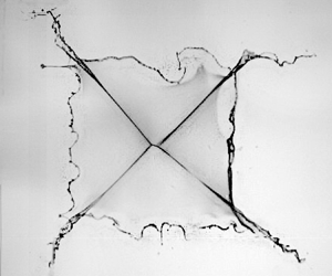
In the course of repeating our earlier experiments to free up soap films from a rectangular wire frame (Mayer & Krechetnikov Reference Mayer and Krechetnikov2010a,Reference Mayer and Krechetnikovb, Reference Mayer and Krechetnikov2017), we encountered the phenomena shown in figure 2, where two outcome patterns can be distinguished: (a) fold and (b) no-fold. While the fold may appear as a standing SW, it proves to be not so. In the fold pattern, SW-like lines along the soap film diagonal are formed shortly (${\sim }1\ \mathrm {ms}$) after the soap film is released from the wire frame. The folds propagate along the diagonal until they merge at the centre of the film (cf. figure 2a). In the no-fold pattern, the soap film simply retracts with the microdroplets dispatched from the soap film boundaries. Notably, the soap film retracts faster in the case of the no-fold pattern, which is especially evident at $6460\ {\mathrm {\mu }}s$ by juxtaposing surface area of the soap films – the distinction being due to different values of soap film thickness.

Figure 2. Fold (a) versus no-fold (b) patterns. (a) Time sequence of the soap film retraction with developing folds along the diagonal of the soap film surface. Soap film solution properties: $0.5\ \mathrm {CMC}$ of $\mathrm {SDS}$, $20\,{\%}\,\mathrm {wt}$ glycerol; soap film thickness and withdrawal velocity are $16.9\ {\mathrm {\mu }}\mathrm {m}$ and $12.4\ \mathrm {mm}\ \mathrm {s}^{-1}$, respectively. (b) Time sequence of the soap film retraction without folds. Soap film solution properties: $1.25\ \mathrm {CMC}$ of $\mathrm {SDS}$, $20\,{\%}\, \mathrm {wt}$ glycerol; soap film thickness and withdrawal velocity are $8.5\ {\mathrm {\mu }}\mathrm {m}$ and $12.4\ \mathrm {mm}\ \mathrm {s}^{-1}$, respectively. The physical image size in both sets of panels is $50\ \mathrm {mm} \times 50\ \mathrm {mm}$.

It is known that the dynamics of the collapsing soap film is dictated by the soap solution properties (viscosity, surface tension, etc.) and the film thickness (Mysels et al. Reference Mysels, Shinoda and Frankel1959; Couder et al. Reference Couder, Chomaz and Rabaud1989; Brenner & Gueyffier Reference Brenner and Gueyffier1999; Savva & Bush Reference Savva and Bush2009). Therefore, a number of experiments were carried out to understand the transition between the fold and no-fold regimes depending upon the values of these parameters in a wide range, though limited by the soap film lifetime necessary to conduct the experiments. For that, the soap solution properties and withdrawal speed were varied as described in § 2. The corresponding maps of the transition in terms of glycerol concentration $C_{g}$ with respect to the soap film thickness $h_{\infty }$ are shown in figure 3. The variation in the soap film thickness along the horizontal axis is due to the change in the bath lowering speed. As evident from this figure by increasing SDS concentration the thickness of the soap film decreases, and the resultant pattern transitions from a fold to a no-fold.

Figure 3. Maps of fold ($\times$) and no-fold ($\square$) patterns with respect to the soap film thickness for five different concentrations of glycerol, $C_g = 5,\ 10,\ 15,\ 20,\ 25\,\%\, wt$ and four concentrations of surfactant: (a) 0.5, (b) 0.75, (c) 1 and (d) 1.25 CMC.

To properly understand the physics underlying the fold to no-fold transition, the data in figure 3 are replotted in figure 4 in the key velocity coordinates. This figure demonstrates the relation between theoretically estimated one-dimensional wave propagation speed $c_{0} = \sqrt {2 E / \rho h_{\infty }}$, arising due to film Marangoni elasticity (Couder et al. Reference Couder, Chomaz and Rabaud1989), and one-dimensional soap film retraction speed $U_{{TC}} = \sqrt {2 \sigma / \rho h_{\infty }}$, calculated based on experimental values of the soap film surface tension $\sigma$, thickness $h_{\infty }$ and elasticity $E=-2\,\mathrm {d}\sigma /\mathrm {d}\ln \varGamma$, where $\varGamma$ is surfactant surface concentration. Data for surface tension $\sigma (\varGamma )$ were extracted from the study of Tajima et al. (Reference Tajima, Muramatsu and Sasaki1970). The use of the formula for elasticity in the Marangoni regime, i.e. when the interface shrinkage only increases the surface surfactant concentration $\varGamma$ without affecting the bulk concentration, is justified by the fact that the characteristic time of the interface shrinkage $t_{{exp}} = l/U_{{TC}} = O(10^{-2}) \ \mathrm {s}$ is much shorter than the characteristic times of desorption $t_{d} = k_{d}^{-1} \sim 0.2 \ \mathrm {s}$ and adsorption $t_{a} = \varGamma / (k_{a} C) \sim 0.2 \ \mathrm {s}$. The values of the adsorption $k_{a} = 0.64 \times 10^{-5}\ \textrm {m}\ \textrm {s}^{-1}$ and desorption $k_{d} = 5.87\ \mathrm {s}^{-1}$ coefficients are calculated via fitting (Fernandez et al. Reference Fernandez, Krechetnikov and Homsy2005) the Langmuir–Hinshelwood equation, $\mathrm {d}\varGamma / \mathrm {d} t = k_{a} C (1 - \theta ) - k_{d} \varGamma$, with $\theta =\varGamma /\varGamma _{m}$ being the fractional coverage and $\varGamma _{m} = 10^{-5}\ \mathrm {mol}\ \mathrm {m}^{-2}$, to the experimental data (Chang & Franses Reference Chang and Franses1992). When the surfactant concentration increases (thus lowering the surface tension) or glycerol concentration decreases (and thus the viscosity as well), the thickness of the soap film decreases and $U_{{TC}}$ approaches $c_{0}$, with the resultant pattern transitioning from fold to no-fold. The solid line in figure 4 corresponding to $c_{0}=U_{{TC}}$ convincingly marks this transition.

Figure 4. Key velocities: theoretically evaluated soap film retraction velocity $U_{{TC}}$ versus elastic wave propagation velocity $c_{0}$. The solid line corresponds to $c_{0}=U_{{TC}}$.

In support of the conclusions drawn from the map in figure 4 – namely, that folds are observed only for $c_{0} > U_{{TC}}$ – two sets of direct measurements of the soap film retraction $U_{{TC}}$ and SW propagation $c_{0}$ speeds were carried out: (i) when the concentration of SDS was fixed at $0.5\ \mathrm {CMC}$ with the concentration of glycerol varied between 5 and 25 % wt in figure 5(a); and (ii) when the concentration of glycerol was set at $20\,{\%}\,\mathrm {wt}$ with the SDS concentration changed in the range 0.5–1.25 CMC in figure 5(b). In both cases, five withdrawal velocities were implemented in the course of the experiments. In figures 5(a) and 5(b) the measured $U_{{TC}}$ and $c_{0}$ are shown with white and black symbols, respectively, confirming that the fold regime corresponds to the condition $c_{0} > U_{{TC}}$. The theoretical estimates of the retraction terminal velocity $U_{{TC}}$ are represented with grey symbols.

Figure 5. Key measured velocities for the case of fold formation. Panels (a) and (b) demonstrate $c_0$ and $U_{{TC}}$ for different soap films. (a) The wave propagation $c_{0}$ and soap film retraction $U_{{TC}}$ velocities for different soap films prepared at $0.5\ \mathrm {CMC}$ of SDS and five concentrations of glycerol ($5$, $10$, $15$, $20$ and $25\,{\%}\,\mathrm {wt}$): for each of them, five different withdrawal velocities were applied, which resulted in $25$ soap film thicknesses. To guide the eye, we added the solid curve $c_0 = \sqrt {2E/{\rho }h_{\infty }}$ fitted to $5$, $10$, $15$ and $20\,{\%}\,\mathrm {wt}$ glycerol data points, yielding $E = 0.182\ \mathrm {N}\ \mathrm {m}^{-1}$ and the dashed curve fitted to $25\,{\%}\,\mathrm {wt}$ glycerol data points, producing $E = 0.121\ \mathrm {N}\ \mathrm {m}^{-1}$. The white and black symbols represent the measured wave propagation and the soap film retraction velocities, respectively. The grey symbols correspond to the theoretically evaluated $U_{{TC}}$. (b) The wave propagation and soap film retraction velocities for different soap films with glycerol concentration fixed at $20\,{\%}\,\mathrm {wt}$. Surfactant concentration is changed in this set of experiments from $0.5$ to $1.25\ \mathrm {CMC}$. The solid line is a fitted curve $c_{0}$ to $0.5$ and $0.625\ \mathrm {CMC}$ data points, yielding $E = 0.186\ \mathrm {N}\ \mathrm {m}^{-1}$; and the dashed line is a fitted curve to $0.75$, $0.875$ and $1\ \mathrm {CMC}$ velocity data points, yielding $E = 0.082\ \mathrm {N}\ \mathrm {m}^{-1}$. At $1.25\ \mathrm {CMC}$ the fold pattern was not observed, and hence data for $c_{0}$ for this concentration cannot be shown in panel (b).

In both figures 5(a) and 5(b), there is some deviation between the theoretical and measured $U_{{TC}}$, which is due to a number of competing factors. First, the film thickens after the SW and hence $U_{{TC}}$ decreases compared to that evaluated at the initial (equilibrium) film thickness $h_{\infty }$ in front of the SW. Second, the surfactant monolayer is compressed between the SW and the retracting edge, thus decreasing the surface tension in this area, compared to the surface tension of the original soap film, and hence $U_{{TC}}$. Third, owing to the difference in surface tension before and after the SW, there is a Marangoni force accelerating the soap film edge and thus increasing $U_{{TC}}$. Given this understanding, in figure 5(a) we can see that, due to the substantial difference between $U_{{TC}}$ and $c_{0}$, the monolayer is not substantially compressed, so that the effect of film thickening after the SW overcomes that of the Marangoni force and hence the theoretical $U_{{TC}}$ overpredicts the measured values. This trend can also be partially discerned in figure 5(b) for $0.5 \ \mathrm {CMC}$ and some of the $0.625 \ \mathrm {CMC}$ points, but for other SDS concentrations, due to weaker compression of the monolayer (as measured by smaller difference between $U_{{TC}}$ and $c_{0}$), film thickening is overtaken by the initially subdominant Marangoni effect leading to higher measured values of $U_{{TC}}$.

Lastly, there is also a concomitant inhibiting effect due to friction between air and the retracting part (aureole) of the soap film as happens in all soap film flows (Couder et al. Reference Couder, Chomaz and Rabaud1989). In our case, however, the dissipation due to the presence of the air phase is negligible, which can be seen from the corresponding ratio of damping forces due to the film (bulk $\mu _{{film}}$ and surface $\mu _{{surface}}$) viscosities and the air viscosity $\mu _{{air}}$, i.e. $F_{{film}}/F_{{air}} \sim 2 \rho _{{air}} \sqrt {\nu _{{air}} U L^{3}} / (\mu _{{film}} h_{\infty } + 2 \mu _{{surface}}) = O(10)$ (cf. formula (39) in Couder et al. Reference Couder, Chomaz and Rabaud1989), evaluated for typical values in our experiments, namely, $L = 5\ \mathrm {cm}$, $U = 5\ \mathrm {m\ s^{-1}}$, $\mu _{{film}} = 10^{3}\ \mathrm {Pa}\ \mathrm {s}$ and $h_{\infty } = 10^{-5}\ \mathrm {m}$. In this formula we took $\mu _{{surface}}$ to be the dilatational surface viscosity $\kappa = 10^{-5}\ \mathrm {N}\ \mathrm {s}\ \mathrm {m}^{-1}$ (Wantke, Fruhner & Örtegren Reference Wantke, Fruhner and Örtegren2003), as most of the surface of the collapsing soap film is subject to dilatation only (Edwards, Brenner & Wasan Reference Edwards, Brenner and Wasan1991), rather than shear (which takes place only near the folds). In any case, dilatation viscosity has the dominant effect compared to that due to the shear $\mu _{s} \approx 5 \times 10^{-6} \ \mathrm {N}\ \mathrm {s}\ \mathrm {m}^{-1}$ and bulk $\mu _{{film}} h_{\infty } \approx 10^{-8} \ \mathrm {N}\ \mathrm {s}\ \mathrm {m}^{-1}$ viscosities. Therefore, for example, the lower measured values of $U_{{TC}}$ compared to the theoretically predicted ones in figure 5(a) are not due to the retarding effect of the air, but primarily are due to the film thickening after the SW compared to the initial (before the soap film release) film thickness.

3.2. Mechanism

The experiments reported above identify the necessary kinematic conditions for the occurrence of folds, but do not address the crux of the problem – the question of the origin of the dynamic folds. The subsonic nature of the folds, $U_{{TC}}< c_{0}$, delineates them from SWs in aerodynamics and hence the underlying mechanism must be different. This becomes obvious from yet another discovered key condition for the observed phenomena: the enigmatic effect of the soap film frame corner when experiments were conducted on frames with sharp (figure 6a) and smoothed out (figure 6b) corners under otherwise the same conditions. Evidently, the curvature of the frame corner directly affects the outcome soap film pattern: the fold pattern is observed for the sharp $90^{\circ }$ corner, while in the case of the smoothed corner no fold pattern is formed in the course of the soap film retraction.

Figure 6. Time sequence of the soap film retraction demonstrating the effect of frame corner (a quarter of the soap film area is shown). In the time sequence shown in (a), the corners of the frame are sharp $90^{\circ }$, while in the set of images shown in (b) the $90^{\circ }$ frame corners are smoothed out. Soap film solution properties: $1\ \mathrm {CMC}$ of $\mathrm {SDS}$, $20\,{\%}\,\mathrm {wt}$ glycerol; the soap film thickness and withdrawal velocity are $10.5\ {\mathrm {\mu }}\mathrm {m}$ and $12.4\ \mathrm {mm}\ \mathrm {s}^{-1}$, respectively. The physical image size is $22\ \mathrm {mm} \times 19\ \mathrm {mm}$.

The appearance of folds, at least visually, might be thought of as related to some sort of buckling. The first candidate is the buckling instability of a sheared thin viscous film, cf. Benjamin & Mullin (Reference Benjamin and Mullin1988) and Slim, Teichman & Mahadevan (Reference Slim, Teichman and Mahadevan2012), to name a few. If one considers a fluid element travelling from the soap film edge towards the diagonal (cf. figure 8c), it is clear that it will experience both rotation $\omega _{z} = ({\partial v}/{\partial x} - {\partial u}/{\partial y})/2$ and shear (strain) $\varepsilon _{xz} = ({\partial v}/{\partial x} + {\partial u}/{\partial y})/2$, though the shear is compensated by rotation as ${\partial v}/{\partial x} = 0$ (note that ${\partial u}/{\partial y} \neq 0$ because $u=0$ before reaching the diagonal and $u=v$ upon reaching it due to symmetry); here $u$ and $v$ are the $x$ and $y$ components of the velocity vector. Despite the fact that shear of the base soap film flow is indeed present at the diagonal, it does not propagate into the interior of the soap film, as is seen from figure 8(a,c) and hence no buckling instability is observed. Moreover, as figure 6(b) demonstrates, when the corner is smoothed out, no folds are formed in spite of the fact that shear must still be present along the diagonal. Hence shear-induced buckling cannot be deemed responsible for fold formation.

Second, the observed wave propagation is closely related to the nature of the surfactant molecules, which have polar and non-polar ends and therefore form a monolayer at the interface between a polar substance such as water and a non-polar one such as air. The surfactant monolayer separates the two substances and reduces surface tension. As happens in our experiments on collapsing soap films, under compression, a surfactant monolayer may experience a mechanical instability, similar to the buckling instability of a beam or a plate, with the wavelength of the surface undulations in the range of $1 - 10 \ \mathrm {\mu }\mathrm {m}$ and amplitude of a few nanometres (Milner, Joanny & Pincus Reference Milner, Joanny and Pincus1989; Saint-Jalmes & Gallet Reference Saint-Jalmes and Gallet1998), which makes them inadequate to explain the observed folds, as the latter apparently have a much larger amplitude. The velocity of the associated wave propagation in surfactant monolayers is dictated by their compressibility (Griesbauer, Wixforth & Schneider Reference Griesbauer, Wixforth and Schneider2009) and could be of the order of $10^{2} \ \mathrm {m}\ \mathrm {s}^{-1}$. While we cannot observe nanometre-amplitude deformations on the soap film surface, the optical properties of the surfactant monolayer change drastically under compression, which may lead to the discernible dark region, i.e. ‘aureole’ (cf. figure 7). Because of the surfactant used in our experiments (SDS), its monolayer compressibility properties (Khattari et al. Reference Khattari, Langer, Aliaskarisohi, Ray and Fischer2011) allow for significantly lower wave propagation speeds $c_{0}$, making them comparable to the edge retraction speeds $U_{{TC}}$, thus enabling the phenomena presented here: transition from no-fold to fold regime. We should also note that for the two concentrations of surfactant ($0.875$ and $1\ \mathrm {CMC}$) an aureole is developed on the soap film surface (figure 7), while for low concentrations ($0.5$ and $0.625\ \mathrm {CMC}$) we have not observed any darkening (figure 2a), though a compressed surfactant monolayer may not always be visible. Yet, the higher SDS concentration $1.25\ \mathrm {CMC}$ implies no SW propagation and hence no aureole (figure 2b), while at low SDS concentrations there are not enough surfactant molecules at the interface to darken the film.

Figure 7. Time sequence of the soap film retraction to show the appearance of a dark region on its surface with the camera zoomed on a quarter of the film area. The dark region develops as the SW propagates on the soap film surface. Soap film solution properties: $0.875\ \mathrm {CMC}$ of $\mathrm {SDS}$, $20\,{\%}\,\mathrm {wt}$ glycerol. Withdrawal velocity and film thickness are $9.1\ \mathrm {mm}\ \mathrm {s}^{-1}$ and $11.4\ {\mathrm {\mu }}\mathrm {m}$, respectively. The physical image size is $22\ \mathrm {mm} \times 19\ \mathrm {mm}$.

4.1. Soap film dynamics

In the Cartesian $(x,y)$ coordinates corresponding to the soap film plane, the continuity and momentum conservation equations governing the soap film dynamics (Wen & Lai Reference Wen and Lai2003) with velocity $\boldsymbol {v}=(u,v)$ and thickness $h(t,x,y)$, written here in analogy to Euler's equations of ideal fluid motion (Landau & Lifshitz Reference Landau and Lifshitz1987), are

(4.1a)$$\begin{gather} \frac{\partial h}{\partial t} + \boldsymbol{\nabla} \boldsymbol{\cdot} (h \boldsymbol{v})= 0, \end{gather}$$

(4.1b)$$\begin{gather}\frac{\partial (h \boldsymbol{v})}{\partial t} + \boldsymbol{\nabla} (h \boldsymbol{v} \otimes \boldsymbol{v} + h \hat{c}^{2} \boldsymbol{\mathsf{I}}) = 0, \end{gather}$$

non-dimensionalized according to

(4.2)\begin{equation} h \rightarrow h_{\infty}h, \quad \boldsymbol{v} \rightarrow v_{\infty} \boldsymbol{v}, \quad x \rightarrow h_{\infty}x, \quad t \rightarrow (h_{\infty} / v_{\infty} ) t, \end{equation}

where $\boldsymbol{\mathsf{I}}$ is the unit tensor and $\hat {c} = c_{0}/v_{\infty }$ is the Marangoni elasticity speed scaled with respect to $v_{\infty } = U_{{TC}}(h_{\infty })$. The existence of an elasticity-mediated speed of propagation, similar to that for sound speed, provides the means for generating SWs in soap films. The presence of the blob along the soap film edge is not crucial for our considerations – there are cases in soap film dynamics when a blob is not formed, for example in highly viscous films (Debrégeas, Martin & Brochard-Wyart Reference Debrégeas, Martin and Brochard-Wyart1995), in which an ‘instantaneous’ thickening of the film is observed due to elastic propagation. Thus the initial and boundary conditions at the soap film edge (rim) for (4.1) are posed, respectively, as

(4.3a)$$\begin{gather} t = 0{:} \quad h(0,x,y)=1; x_{r}=0, u_{r}=1; y_{r}=0, v_{r}=1; \end{gather}$$

(4.3b)$$\begin{gather}x = x_{r}(t){:} \quad u_{r} = \sqrt{h_{\infty} /h_{r}}; \quad y = y_{r}(t){:} \quad v_{r} = \sqrt{h_{\infty} /h_{r}}; \end{gather}$$

above we have taken into account that the blob-free soap film rim moves with the speed $U_{{TC}}(h_{r})$ corresponding to the film thickness $h_{r}$ at the rim.

For numerical implementation, (4.1) can be rewritten as

(4.4)\begin{equation} W_t + G(W)_x + H(W)_y = 0, \end{equation}

where $G$ and $H$ are nonlinear functions of $W$:

(4.5a–c)\begin{equation} W = \begin{bmatrix} h\\ hu\\ hv \end{bmatrix},\quad G = \begin{bmatrix} hu\\ hu^2+F\\ huv \end{bmatrix},\quad H = \begin{bmatrix} hv\\ huv\\ hv^2+F \end{bmatrix}. \end{equation}

In order to numerically integrate this two-dimensional soap film model, it is discretized as appropriate for solving nonlinear systems of hyperbolic conservative equations (Toro Reference Toro1999) using finite differences with a backward scheme. First we integrate (4.4) by sweeping in the $x$ direction,

(4.6)\begin{equation} W_{i,j}^{n+{1}/{2}} = W_{i,j}^{n} +\frac{\Delta t}{\Delta x} (G_{i-1,j}^{n}-G_{i,j}^{n} ), \end{equation}

and then, as is common in splitting schemes (Toro Reference Toro1999), sweeping in the $y$ direction,

(4.7)\begin{equation} W_{i,j}^{n+1} = W_{i,j}^{n+{1}/{2}} + \frac{\Delta t}{\Delta y} (H_{i,j-1}^{n}-H_{i,j}^{n} ); \end{equation}

here the index $n$ stands for the time stamp and indices $i$ and $j$ for mesh numbers in the $x$ and $y$ directions, respectively. For the system of equations (4.4), the Courant condition

(4.8)\begin{equation} \frac{\Delta t \max{u}}{\Delta x} + \frac{\Delta t \max{v}}{\Delta y}<1 \end{equation}

allows one to choose the time step $\Delta t$ as well as the spatial steps $\Delta x$ and $\Delta y$ in the $x$ and $y$ directions, respectively. The results of the numerical simulation after performing $80$ time steps are reported in figure 8(c,d).

Figure 8. Experiments versus theory. (a) PIV velocity field acquired $2.4\ \mathrm {ms}$ after the triggering pulse. The time difference between the two PIV images is $100\ {\mathrm {\mu }}\mathrm {s}$. The size of the grey area is $19.8\ \mathrm {mm} \times 22\ \mathrm {mm}$. The experimentally measured one-dimensional shock and retraction velocities are $c_0 = 4.02 \ \mathrm {m}\ \mathrm {s}^{-1}$ and $U_{{TC}} = 1.86 \ \mathrm {m}\ \mathrm {s}^{-1}$, respectively. (b) Fold formation on the soap film $2.6\ \mathrm {ms}$ after the triggering pulse. The physical image size is $22\ \mathrm {mm} \times 22\ \mathrm {mm}$. The soap solution in (a,b) consists of ultrapure water, $20\,{\%}\,\mathrm {wt}$ glycerol and $0.5\ \mathrm {CMC}$ of SDS. The soap film thickness and withdrawal velocity are $16.9\ \mathrm {\mu }\mathrm {m}$ and $12.4\ \mathrm {mm}\ \mathrm {s}^{-1}$, respectively. (c) Numerical result for the velocity field distribution on the soap film in the presence of fold. (d) Contour plot of numerically calculated $h(t,x,y)$ for the conditions corresponding to those in panel (c).

Modelling based on numerical implementation of (4.1) and (4.3) shows that the computed velocity field distribution in figure 8(c) is in good agreement with the experimental PIV measurements in figure 8(a). In figure 8(c), $\hat {c}=2.3$ was chosen to fit the kinematics in figure 8(a), which is close to the experimental value $\hat {c} = 2.16$. A contour plot of the numerical solution of (4.1) and (4.3) for the film thickness $h(t,x,y)$ demonstrates a fold on the diagonal of the soap film as a result of wave propagation ahead of the retracting edge (cf. figure 8d) in analogy to the experimental observations in figure 8(b).

4.2. Shock wave speed

For convenience, here we consider the dimensional version of (4.1) with $c$ being the elastic wave speed. When integrated across the surface of discontinuity, the mass conservation equation (4.1a) yields $[h v]_{1}^{2}=0$ for the difference in mass flux on either side of the SW (cf. figure 9a), which in the frame of reference associated with the moving SW (cf. figure 9b) reads (Landau & Lifshitz Reference Landau and Lifshitz1987)

(4.9)\begin{equation} c h_{\infty} = h_{-} (c-v_{-} ); \end{equation}

in this formula, on the left-hand side, $c$ plays the role of the velocity of the soap film of thickness $h_{\infty }$ incoming onto (in front of) the SW, while, on the right-hand side, $c-v_{-}$ is the soap film velocity behind the SW and the corresponding soap film thickness is $h_{-}$. Equation (4.9) signifies some important properties: one must have $c>v_{-}$ and $h_{-} \neq h_{\infty }$. To (4.9) we should add a momentum conservation condition following from the conservative form of the differential momentum conservation equation (4.1b), i.e. $[h (v^{2} + c^{2})]_{1}^{2} = 0$ in the frame of reference moving with the SW, thus producing

(4.10)\begin{equation} h_{\infty} (c^{2} + c_{\infty} ) = h_{-}[(c-v_{-})^{2} + c_{-}^{2}], \end{equation}

where we took into account that in general the SW speed $c$ is different from the sound speed $c_{\infty }$ in front of the SW and from $c_{-}$ behind it. By eliminating $c-v_{-}$ from (4.9) and (4.10), we find the (squared) SW speed

(4.11)\begin{equation} c^{2} = \frac{h_{-}}{h_{\infty}} \, \frac{h_{-} c_{-}^{2} - h_{\infty} c_{\infty}^{2}}{h_{-}-h_{\infty}}, \end{equation}

which tells us that, if the sound speed is calculated as for elastic waves, i.e. $c_{\infty } = \sqrt {E/\rho h_{\infty }}$ and similarly for $c_{-}$, then SW cannot form unless the elasticities $E_{\infty }$ in front of and $E_{-}$ behind the SW are different.

Figure 9. SW propagation in the laboratory (a) and moving (b) frames of reference.

4.3. Dynamics on the diagonal

While the numerical solution in § 4.1 replicates the experimental observations, it does not provide deeper insights offered by an analytical study. To that end, using (4.1) we derive the Rankine–Hugoniot conditions analogous to SWs in aerodynamics (Landau & Lifshitz Reference Landau and Lifshitz1987) along the soap film diagonal $\varGamma$ defined by $x=y$, where a fold is observed:

(4.12a)$$\begin{gather} [h u]_{1}^{2} \frac{\mathrm{d} y}{\mathrm{d}\kern0.7pt x} = [h v]_{1}^{2}, \end{gather}$$

(4.12b)$$\begin{gather}\left[h\boldsymbol{v}u + h \hat{c}^{2}I_{x}\right]_{1}^{2} \frac{\mathrm{d} y}{\mathrm{d}\kern0.7pt x} = [h \boldsymbol{v} v + h \hat{c}^{2} I_{y} ]_{1}^{2}; \end{gather}$$

with the notation introduced $1$ is the phase below and $2$ above the diagonal (cf. figure 8c), $I_{x} = (1,\,0)^\textrm {T}$ and $I_{y} = (0,\,1)^\textrm {T}$. The analysis of (4.12) leads to

(4.13)\begin{equation} u_{1} = v_{1}, \quad u_{2} = v_{2}, \quad h_{1} = h_{2}, \quad (\boldsymbol{\nabla} h )_{1} = (\boldsymbol{\nabla} h )_{2}, \end{equation}

which are the natural conditions across the diagonal $\varGamma$ due to the symmetry of the problem with respect to it. Effectively, the diagonal serves as an impermeable wall or, in fact, two impermeable walls in between which (on a set of measure zero) there exists a dynamics mostly independent of the rest of the soap film, because the initial perturbation of large enough amplitude at the corner is confined by the soap film flows on either side, and hence can evolve only along the diagonal without propagating sidewise. On the other hand, any perturbation coming from the edge of the soap film away from the corner decays quickly due to being non-confined. Since the diagonal has its own dynamics, it must be governed by the corresponding equations, which are naturally the same soap film equations (4.1), but collapsed on the diagonal. Since the system (4.1) is in a coordinate-free form, the equations on the diagonal straightforwardly follow from substitution of the gradient $\boldsymbol {\nabla }$ by the directional derivative $\partial / \partial _{\varGamma }$ along the diagonal $\varGamma$, analogous in spirit to Hadamard's method of descent (Hadamard Reference Hadamard1923).

Moreover, the diagonal proves to be one of the characteristics. Indeed, the characteristic surface $\varOmega (t,x,y)$ in the space of independent variables $(t,x,y)$ is defined in the context of proving the Cauchy–Kovalevskaya theorem: namely, an initial value (Cauchy) problem does not have a unique solution, and thus is ill-posed, if the initial data are given at $\varOmega (t,x,y)$. This allows a straightforward determination of the characteristic surface by making a transformation from the original independent variables $(t,x,y)$ to $\varOmega (t,x,y)$, in which resolution of the governing partial differential equations (4.1) for the highest-order derivatives of the solution becomes impossible (Petrovsky Reference Petrovsky1954):

(4.14)\begin{equation} \begin{pmatrix} \varDelta & h \varOmega_{x} & h \varOmega_{y}\\ c^{2} \varOmega_{x} & h \varDelta & 0\\ c^{2} \varOmega_{y} & 0 & h \varDelta \end{pmatrix} \begin{pmatrix} h_{\varOmega}\\ u_{\varOmega}\\ v_{\varOmega} \end{pmatrix} = 0, \end{equation}

where $\varDelta = \varOmega _{t} + u \varOmega _{x} + v \varOmega _{y}$. Hence, the characteristic determinant reads

(4.15)\begin{equation} h^{2} \varDelta [\varDelta^{2} - c^{2} (\varOmega_{x}^{2} + \varOmega_{y}^{2} )] = 0, \end{equation}

implying that the system (4.1) is hyperbolic with one of the characteristics being the instantaneous streamline $\varOmega _{t} + u \varOmega _{x} + v \varOmega _{y} = 0$ – the diagonal $\varGamma$ is one of them – while the other ones are dictated by the soap film ‘compressibility’ with some correction terms:

(4.16)\begin{equation} \varOmega_{t}^{2} + (u^{2}-c^{2}) \varOmega_{x}^{2} + (v^{2}-c^{2}) \varOmega_{y}^{2} + u \varOmega_{x} (\varOmega_{t} - \tfrac{1}{2} v \varOmega_{y} ) + v \varOmega_{y} (\varOmega_{t} - \tfrac{1}{2} u \varOmega_{x} ) = 0. \end{equation}

4.4. Acoustic effects

Further insights into the origin of folds can be gained with the help of geometric acoustics, the basic assumption of which (Landau & Lifshitz Reference Landau and Lifshitz1987) is that locally a sound wave $\phi (t,\boldsymbol {r}) = A(t,\boldsymbol {r}) \, \textrm {e}^{\mathrm {i} \psi (t,\boldsymbol {r})}$ with the wavevector $\boldsymbol {k} = \boldsymbol {\nabla } \psi$ and frequency $\omega = - {\partial \psi / \partial t}$ can be considered plane (cf. figure 11a), provided the amplitude $A$ and the wave direction $\boldsymbol {k}$ do not change appreciably over the sound wavelength $\lambda = 2{\rm \pi} /|\boldsymbol {k}|$, i.e. $\lambda /L \ll 1$ relative to the characteristic length scale $L$ of the phenomena at hand (the soap film span). Let us try to understand the fold formation in the soap film dynamics with the help of a single eikonal equation, which relates $\omega$ and $\boldsymbol {k}$ and is known to admit multivalued solutions corresponding to caustics. Taking into account the motion of the soap film itself (Kritikos Reference Kritikos1967) with the velocity field $\boldsymbol {v}=(u,v)$ furnishes

(4.17)\begin{equation} \omega = c_{0} |\boldsymbol{k}| + \boldsymbol{v} \boldsymbol{\cdot} \boldsymbol{k}, \end{equation}

which is a modification of the steady-state eikonal equation (Landau & Lifshitz Reference Landau and Lifshitz1987) $|\boldsymbol {k}|^{2} = \omega ^{2}/c_{0}^{2}$. While the general case $|\boldsymbol {v}| \sim c_{0}$ can be formally considered, in order to make the implications of the presence of the soap film flow transparent, let us treat the limit $|\boldsymbol {v}| \ll c_{0}$. Using the standard characteristic analysis for the first-order nonlinear partial differential equations (Zauderer Reference Zauderer2006), we arrive at the acoustic ray equation:

(4.18)\begin{equation} \frac{1}{2} \frac{\mathrm{d}^{2} \boldsymbol{r}}{\mathrm{d} s^{2}} = \boldsymbol{\nabla} (n^{2}) + \boldsymbol{\nabla} n \, \boldsymbol{t} \boldsymbol{\cdot} \boldsymbol{v} + n \, \boldsymbol{t} \boldsymbol{\cdot} \boldsymbol{\nabla} \boldsymbol{v} + \frac{\mathrm{d}}{\mathrm{d} s} (n \boldsymbol{v} ); \end{equation}

above the velocity vector is scaled as $\boldsymbol {v} \rightarrow \boldsymbol {v}/c_{0}$, $\boldsymbol {t} = \mathrm {d} \boldsymbol {r} / \mathrm {d} s$ is the vector tangent to the ray, $s$ the arclength, $n=\omega /c_{0}$ the refractive index and $\boldsymbol {t} \boldsymbol {\cdot } \boldsymbol {\nabla } \boldsymbol {v}$ the usual vector–tensor product:

(4.19)\begin{equation} \boldsymbol{t} \boldsymbol{\cdot} \boldsymbol{\nabla} \boldsymbol{v} = (x_{s},y_{s} ) \left( \begin{array}{cc} u_{x} & u_{y} \\ v_{x} & v_{y} \end{array} \right) = x_{s} (\boldsymbol{i} u_{x} + \boldsymbol{j} u_{y}) + y_{s} (\boldsymbol{i} v_{x} + \boldsymbol{j} v_{y}). \end{equation}

The first term on the right-hand side of (4.18) is responsible for the ray bending in the direction of decreasing sound speed $c_{0}$ or, equivalently, in the direction of increasing refractive index $n$. Since $|\mathrm {d}^{2} \boldsymbol {r} / \mathrm {d} s^{2}| = \kappa (s)$ is the curvature of the ray, then, in the presence of an inhomogeneous refractive index $n=n(x,y)$, the ray bends in the direction of the gradient $\boldsymbol {\nabla } n$ (e.g. for the ray in figure 8(c) the vector $\boldsymbol {\nabla } n$ points towards the diagonal). On the soap film diagonal $\varGamma$, $\boldsymbol {\nabla } n$ is discontinuous and thus the curvature $\kappa (s)$ is singular. While the first term on the right-hand side of (4.18) is of the potential field nature due to its gradient structure, the last three terms, when rewritten in the tensor notation and recalling that $\mathrm {d} / \mathrm {d} s = \boldsymbol {t} \boldsymbol {\cdot } \boldsymbol {\nabla }$, can be combined as

(4.20)\begin{equation} \boldsymbol{\nabla}_{j} n t_{i} u^{i} + n t_{i} \boldsymbol{\nabla}_{j} u^{i} + t^{i} \boldsymbol{\nabla}_{i} (n u_{j}) = t^{i}[\boldsymbol{\nabla}_{j}(n u_{i}) + \boldsymbol{\nabla}_{i} (n u_{j})], \end{equation}

where we have taken into account that the gradient $\boldsymbol {\nabla }$ is a covariant vector, while the velocity $\boldsymbol {v}$ is contravariant; lowering or raising the index is done with the help of a metric tensor $\boldsymbol {g}$, e.g. $g^{ij} t_{i} = t^{\,j}$. The expression in parentheses on the right-hand side of (4.20) can be recognized as the in-plane symmetric stress tensor $\tau _{ij} \equiv \boldsymbol {\nabla }_{j}(n u_{i}) + \boldsymbol {\nabla }_{i} (n u_{j})$, though weighted with the refractive index $n$. Since the latter is positive, the dynamic effect of (4.20) on acoustic rays is mostly determined by the flow field $\boldsymbol {v}$ in the soap film, with the meaning of (4.20) being essentially the total force (in the soap film plane) acting on the oriented unit area with the normal $\boldsymbol {t}$. Because the velocity gradient $\boldsymbol {\nabla }_{j} u_{i}$ in (4.20) is negligibly small away from the diagonal, the effect of the first term on the right-hand side of (4.18) is dominant.

In summary, all the considered acoustic effects – ‘sound’ speed $c_{0}$ decreasing towards the diagonal (since the film thickness $h$ is larger there) as well as the soap film flow $\boldsymbol {v}$ – suggest that the acoustic rays will bend towards the diagonal of the soap film (§ 4.4).