


1 Introduction
Mach reflection is an important phenomenon in steady supersonic flow (Mach Reference Mach1878; Ben-Dor Reference Ben-Dor2007). As shown in figure 1, this reflection has a triple shock point (T) which connects the incident shock wave
 $(i)$
, the reflected shock wave
$(i)$
, the reflected shock wave
 $(r)$
, the Mach stem
$(r)$
, the Mach stem
 $(m)$
and the slipline
$(m)$
and the slipline
 $(s)$
. von Neumann (Reference von Neumann1943) provided the criteria for transition to Mach reflection from regular reflection, the latter involves only an incident shock wave and a reflected shock wave. Precisely, for a given inflow Mach number
$(s)$
. von Neumann (Reference von Neumann1943) provided the criteria for transition to Mach reflection from regular reflection, the latter involves only an incident shock wave and a reflected shock wave. Precisely, for a given inflow Mach number
 $M_{0}$
, if the wedge angle
$M_{0}$
, if the wedge angle
 $\unicode[STIX]{x1D703}_{w}$
(the deflection angle of flow across the incident shock wave) is large enough so that the reflected shock wave detaches, we necessarily have Mach reflection (called detachment criterion). If this angle is low enough so that the pressure increase across the reflected shock wave can not be balanced by the pressure increase across the Mach stem, then we necessarily have regular reflection (called mechanical equilibrium or von Neumann criterion). In the plane
$\unicode[STIX]{x1D703}_{w}$
(the deflection angle of flow across the incident shock wave) is large enough so that the reflected shock wave detaches, we necessarily have Mach reflection (called detachment criterion). If this angle is low enough so that the pressure increase across the reflected shock wave can not be balanced by the pressure increase across the Mach stem, then we necessarily have regular reflection (called mechanical equilibrium or von Neumann criterion). In the plane
 $(M_{0},\unicode[STIX]{x1D703}_{w})$
these two criteria enclose a region, called the dual solution domain, for which both reflections may be possible (Henderson & Lozzi Reference Henderson and Lozzi1975; Hornung, Oertel & Sandeman Reference Hornung, Oertel and Sandeman1979). The existence of both types of reflection in the dual solution domain has been verified theoretically (Teshukov Reference Teshukov1989; Li & Ben-Dor Reference Li and Ben-Dor1996), numerically (Vuillon, Zeitoun & Ben-Dor Reference Vuillon, Zeitoun and Ben-Dor1995) and experimentally (Chpoun et al.
Reference Chpoun, Passerel, Li and Ben-Dor1995). In the dual solution domain, whether we have Mach reflection or regular reflection depends on the history of the building of the actual steady flow. Hysteresis of the reflection type and solution occurs when changing the wedge angle or inflow Mach number from different directions (see Ben-Dor et al. (Reference Ben-Dor, Ivanov, Vasilev and Elperin2002) and Hornung (Reference Hornung2014) for a review of important works related to this subject).
$(M_{0},\unicode[STIX]{x1D703}_{w})$
these two criteria enclose a region, called the dual solution domain, for which both reflections may be possible (Henderson & Lozzi Reference Henderson and Lozzi1975; Hornung, Oertel & Sandeman Reference Hornung, Oertel and Sandeman1979). The existence of both types of reflection in the dual solution domain has been verified theoretically (Teshukov Reference Teshukov1989; Li & Ben-Dor Reference Li and Ben-Dor1996), numerically (Vuillon, Zeitoun & Ben-Dor Reference Vuillon, Zeitoun and Ben-Dor1995) and experimentally (Chpoun et al.
Reference Chpoun, Passerel, Li and Ben-Dor1995). In the dual solution domain, whether we have Mach reflection or regular reflection depends on the history of the building of the actual steady flow. Hysteresis of the reflection type and solution occurs when changing the wedge angle or inflow Mach number from different directions (see Ben-Dor et al. (Reference Ben-Dor, Ivanov, Vasilev and Elperin2002) and Hornung (Reference Hornung2014) for a review of important works related to this subject).

Figure 1. Mach reflection. The inflow Mach number
 $M_{0}$
, the wedge angle
$M_{0}$
, the wedge angle
 $\unicode[STIX]{x1D703}_{w}$
, the height
$\unicode[STIX]{x1D703}_{w}$
, the height
 $H_{A}$
and the lower wedge surface length
$H_{A}$
and the lower wedge surface length
 $w$
are given conditions. This reflection produces an incident shock wave (
$w$
are given conditions. This reflection produces an incident shock wave (
 $i$
), a reflected shock wave (
$i$
), a reflected shock wave (
 $r$
) composed of a straight segment (TF), a curved segment (FK) and another straight segment (
$r$
) composed of a straight segment (TF), a curved segment (FK) and another straight segment (
 $r^{^{\prime }}$
), a strong shock wave called the Mach stem (
$r^{^{\prime }}$
), a strong shock wave called the Mach stem (
 $m$
) and a slipline (
$m$
) and a slipline (
 $s$
) (composed of a free segment TB and an interactive segment BDE, the dashed line emanating from the triple point is a straight line tangent to the slipline at point T). These four discontinuities are connected by the triple point T. The wedge rear corner R produces an expansion fan (with Mach waves
$s$
) (composed of a free segment TB and an interactive segment BDE, the dashed line emanating from the triple point is a straight line tangent to the slipline at point T). These four discontinuities are connected by the triple point T. The wedge rear corner R produces an expansion fan (with Mach waves
 $R_{c}$
) and the transmitted expansion waves (
$R_{c}$
) and the transmitted expansion waves (
 $R_{t}$
) come from the interaction of this expansion fan with the reflected shock wave. The flow between the slipline and the reflecting surface is quasi-one-dimensional and is composed of a subsonic pocket (before the sonic throat D) and a supersonic pocket (after D).
$R_{t}$
) come from the interaction of this expansion fan with the reflected shock wave. The flow between the slipline and the reflecting surface is quasi-one-dimensional and is composed of a subsonic pocket (before the sonic throat D) and a supersonic pocket (after D).
One important issue for Mach reflection is to find an analytical solution in some uniform flow regions. Giving the flow parameters
 $M_{0},p_{0}$
(pressure),
$M_{0},p_{0}$
(pressure),
 $T_{0}$
(temperature) and the wedge angle
$T_{0}$
(temperature) and the wedge angle
 $\unicode[STIX]{x1D703}_{w}$
, the classical oblique shock wave solution gives the solution for the incident shock wave, and the solution inside the expansion fan and above the reflected shock wave follows from the Prandtl–Meyer relations. The three-shock theory of von Neumann (Reference von Neumann1945) gives the solution of flow parameters very near the triple point, including the directions or angles of the reflected shock and slipline at the triple point. Near the triple point, the three shock waves and slipline separate the flow into four regions (figure 1): region (0) is upstream of the Mach stem and the incident shock wave, region (1) is between the incident shock wave and the reflected shock wave, region (2) is downstream of the reflected shock wave, and region (3) is downstream of the Mach stem. Below we shall use the subscript
$\unicode[STIX]{x1D703}_{w}$
, the classical oblique shock wave solution gives the solution for the incident shock wave, and the solution inside the expansion fan and above the reflected shock wave follows from the Prandtl–Meyer relations. The three-shock theory of von Neumann (Reference von Neumann1945) gives the solution of flow parameters very near the triple point, including the directions or angles of the reflected shock and slipline at the triple point. Near the triple point, the three shock waves and slipline separate the flow into four regions (figure 1): region (0) is upstream of the Mach stem and the incident shock wave, region (1) is between the incident shock wave and the reflected shock wave, region (2) is downstream of the reflected shock wave, and region (3) is downstream of the Mach stem. Below we shall use the subscript
 $k$
to denote solutions in region (
$k$
to denote solutions in region (
 $k$
) and the superscript
$k$
) and the superscript
 $T$
to denote solutions very close to the triple point T (see figure 2
a). For instance,
$T$
to denote solutions very close to the triple point T (see figure 2
a). For instance,
 $M_{3}^{T}$
is the Mach number in region (3) in the neighbourhood of the triple point.
$M_{3}^{T}$
is the Mach number in region (3) in the neighbourhood of the triple point.

Figure 2. (a) Near the triple point the solutions in (1), (2) and (3) are given by the three-shock theory independent of the Mach stem height. (b) Secondary Mach waves are produced over the slipline to balance the pressure decrease below the slipline (Gao & Wu Reference Gao and Wu2010).
Apart from the flow close to the triple point which can be easily solved by the three-shock theory, the flow in other regions involves complex structures. For instance, the reflected shock wave is subjected to the interaction of the expansion fan from the wedge trailing edge (R), and this interaction curves the reflected shock wave. After transmitting the reflected shock wave, the expansion waves, called transmitted expansion waves, intersect the slipline so that the quasi-one-dimensional duct formed by the slipline (TBCDE) and the reflecting surface is similar to a Laval nozzle, with a sonic throat (D) upstream of which the flow is subsonic (
 $M_{3}<1$
) and downstream of which the flow is supersonic (
$M_{3}<1$
) and downstream of which the flow is supersonic (
 $M_{6}>1$
). The Mach stem is also curved.
$M_{6}>1$
). The Mach stem is also curved.
The second issue of interest is the shape of the Mach stem and of the interacting part of the reflected shock wave. Li & Ben-Dor (Reference Li and Ben-Dor1997) modelled the Mach stem using a second-order curve. By assuming the Mach stem to be only slightly curved with respect to a normal shock wave, Tan, Ren & Wu (Reference Tan, Ren and Wu2006) built a small perturbation theory for the flow just behind the Mach stem and proved that the Mach stem can be approximated by a circular arc centred on the reflecting surface. The shape of the reflected shock wave can be analysed by the shock-expansion wave interaction method of Rosciszewski (Reference Rosciszewski1960) and Hasimoto (Reference Hasimoto1964), or by the approximate method of Li & Ben-Dor (Reference Li and Ben-Dor1995). However, even the initial point (point F in figure 1) of the interacting part of the reflected shock wave depends not only on the inlet height
 $H_{A}$
and length
$H_{A}$
and length
 $w$
of the lower surface of the wedge, but also on the Mach stem height
$w$
of the lower surface of the wedge, but also on the Mach stem height
 $H_{T}$
, the latter is also unknown.
$H_{T}$
, the latter is also unknown.
The third important issue is the mechanism by which the size of a Mach reflection is determined, as raised by Courant & Friedrichs (Reference Courant and Friedrichs1948) and Liepmann & Roshko (Reference Liepmann and Roshko1957). Though Hornung & Robinson (Reference Hornung and Robinson1982) performed experimental measurements of the Mach stem height, this question was considered to be one of the unsolved shock wave reflection problems before the 1990s, as pointed out by Emanuel (Reference Emanuel1986), Ben-Dor & Takayama (Reference Ben-Dor and Takayama1992) and Li & Ben-Dor (Reference Li and Ben-Dor1997). Physical models have then been proposed for predicting the Mach stem height (Azevedo & Liu Reference Azevedo and Liu1993; Li & Ben-Dor Reference Li and Ben-Dor1997; Mouton & Hornung Reference Mouton and Hornung2007; Gao & Wu Reference Gao and Wu2010). In the model of Azevedo & Liu (Reference Azevedo and Liu1993), the sonic throat is assumed to be at the turning point (B, where the leading characteristics of the transmitted expansion waves intersects the slipline), while Li & Ben-Dor (Reference Li and Ben-Dor1997) allowed the sonic throat to be determined by the transmitted expansion waves and concluded that the expansion fan due to the wedge determines the size and location of the Mach stem by creating the sonic throat and carrying information on the upper geometrical conditions through the subsonic pocket to the Mach stem. Mouton & Hornung (Reference Mouton and Hornung2007) improved the model of Azevedo & Liu (Reference Azevedo and Liu1993) by allowing the sonic throat to occur further downstream, but assumed the slipline to be straight. In the work of Azevedo & Liu (Reference Azevedo and Liu1993), Li & Ben-Dor (Reference Li and Ben-Dor1997) and Mouton & Hornung (Reference Mouton and Hornung2007), the slipline ahead the point B is treated as a straight line.
Based on a close examination of the numerical results by computational fluid dynamics (CFD), Gao & Wu (Reference Gao and Wu2010) found that the flow just behind the leading part of the reflected shock wave is not a uniform one. They argued that due to the pressure decrease below the slipline (a subsonic convergent duct has a pressure decrease), there must be a series of expansion waves over the free part of the slipline (i.e., slipline before point B), see figure 2(b) for illustration. By taking into account these expansion waves and by further assuming reflected compression waves over the interacting part of the slipline (i.e., slipline after point B), they predicted Mach stem heights which are closer to CFD results than the methods by Azevedo & Liu (Reference Azevedo and Liu1993), Li & Ben-Dor (Reference Li and Ben-Dor1997) and Mouton & Hornung (Reference Mouton and Hornung2007). Gao & Wu (Reference Gao and Wu2010) also provided the shape of the reflected shock wave and slipline and found that point B is an inflection point, where the height and slope of the slipline are continuous.
However, Gao & Wu (Reference Gao and Wu2010) used a point-wise wave interaction model, which treats the reflected shock wave, the slipline and the Mach waves as discrete elements (i.e., any curved wave is decomposed into a finite number of straight segments) and computed the flow using a finite number of shock/Mach wave or Mach wave/slipline interaction algorithms. Such a method is complicated to implement and time-consuming. Second, due to the discrete nature of this treatment, it can not predict slope discontinuity of the slipline, if this discontinuity exists somewhere.
Figure 3 shows the density contour lines obtained by Gao & Wu (Reference Gao and Wu2010, figure 4) for
 $M_{0}=4.5$
,
$M_{0}=4.5$
,
 $\unicode[STIX]{x1D703}_{w}=25^{\circ }$
and
$\unicode[STIX]{x1D703}_{w}=25^{\circ }$
and
 $w/H_{A}=1.1$
. We observe a noticeable change of direction of the contourlines across the curve
$w/H_{A}=1.1$
. We observe a noticeable change of direction of the contourlines across the curve
 $\text{BB}^{\prime }$
issuing from point B. Here this change of direction is for contours of density. For contours of pressure and Mach number, not displayed here, we observe a similar change of direction across
$\text{BB}^{\prime }$
issuing from point B. Here this change of direction is for contours of density. For contours of pressure and Mach number, not displayed here, we observe a similar change of direction across
 $\text{BB}^{\prime }$
. The phenomenon of this change of direection is also seen in other numerical results, see for instance Ben-Dor et al. (Reference Ben-Dor, Ivanov, Vasilev and Elperin2002, figures 5 and 9) and Gao & Wu (Reference Gao and Wu2010, figures 4 and 5).
$\text{BB}^{\prime }$
. The phenomenon of this change of direection is also seen in other numerical results, see for instance Ben-Dor et al. (Reference Ben-Dor, Ivanov, Vasilev and Elperin2002, figures 5 and 9) and Gao & Wu (Reference Gao and Wu2010, figures 4 and 5).
The change of direction of contourlines of flow parameters indicates the existence of a susceptible compression wave or weak shock wave. The hypothetical shock wave should come from a discontinuity of the slope of the slipline at the turning point B. However, if such a discontinuity exists, it is difficult to capture it numerically or by a point-wise wave interaction model. To verify this and to have a more physical model for prediction of the Mach stem height and shape of the slipline and reflected shock waves, we derive in this paper analytical expressions for the shape of the reflected shock wave and slipline. The theory will be given in § 2 and results are presented in § 3. Conclusions will be summarized in § 4.

Figure 3. Density contours for
 $M_{0}=4.5$
,
$M_{0}=4.5$
,
 $\unicode[STIX]{x1D703}_{w}=25^{\circ }$
and
$\unicode[STIX]{x1D703}_{w}=25^{\circ }$
and
 $w/H_{A}=1.1$
. There is a noticeable change of direction of contour lines across the curve
$w/H_{A}=1.1$
. There is a noticeable change of direction of contour lines across the curve
 $\text{BB}^{\prime }$
.
$\text{BB}^{\prime }$
.
2 Analytical solution of the slipline, reflected shock wave and global algorithm for the Mach stem height
Given
 $M_{0}$
and
$M_{0}$
and
 $\unicode[STIX]{x1D703}_{w}$
, the use of the oblique shock wave relation gives the solution in the uniform region (1) and the three-shock theory of von Neumann (Reference von Neumann1945) gives the Mach numbers
$\unicode[STIX]{x1D703}_{w}$
, the use of the oblique shock wave relation gives the solution in the uniform region (1) and the three-shock theory of von Neumann (Reference von Neumann1945) gives the Mach numbers
 $M_{2}^{T},M_{3}^{T}$
, pressures
$M_{2}^{T},M_{3}^{T}$
, pressures
 $p_{2}^{T}=p_{3}^{T}$
, the initial shock angle
$p_{2}^{T}=p_{3}^{T}$
, the initial shock angle
 $\unicode[STIX]{x1D6FD}_{r}^{T}$
of the reflected shock wave and the initial angle of the slipline
$\unicode[STIX]{x1D6FD}_{r}^{T}$
of the reflected shock wave and the initial angle of the slipline
 $\unicode[STIX]{x1D6FF}_{s}^{T}$
. The method will be given by first assuming a Mach stem height
$\unicode[STIX]{x1D6FF}_{s}^{T}$
. The method will be given by first assuming a Mach stem height
 $H_{T}$
. The global algorithm to find
$H_{T}$
. The global algorithm to find
 $H_{T}$
will be given in § 2.4. Define
$H_{T}$
will be given in § 2.4. Define
 $\unicode[STIX]{x1D717}(M)$
and
$\unicode[STIX]{x1D717}(M)$
and
 $\unicode[STIX]{x1D708}(M)$
by
$\unicode[STIX]{x1D708}(M)$
by
 $$\begin{eqnarray}\displaystyle \left.\begin{array}{@{}c@{}}\displaystyle \unicode[STIX]{x1D717}(M)=1+\frac{\unicode[STIX]{x1D6FE}-1}{2}M^{2}\\ \displaystyle \unicode[STIX]{x1D708}(M)=\sqrt{\frac{\unicode[STIX]{x1D6FE}+1}{\unicode[STIX]{x1D6FE}-1}}\arctan \sqrt{\frac{\unicode[STIX]{x1D6FE}-1}{\unicode[STIX]{x1D6FE}+1}(M^{2}-1)}-\arctan \sqrt{M^{2}-1}.\end{array}\right\} & & \displaystyle\end{eqnarray}$$
Here
 $\unicode[STIX]{x1D708}(M)$
is the Prandtl–Meyer function and
$\unicode[STIX]{x1D708}(M)$
is the Prandtl–Meyer function and
 $\unicode[STIX]{x1D6FE}$
is the ratio of specific heats. The function
$\unicode[STIX]{x1D6FE}$
is the ratio of specific heats. The function
 $\unicode[STIX]{x1D717}(M)$
is a factor of isentropic relation that appears on many occasions.
$\unicode[STIX]{x1D717}(M)$
is a factor of isentropic relation that appears on many occasions.
2.1 Shape of the free part of the slipline
The free part TB of the slipline (figures 1 and 2 b) had been treated as a straight line until Gao & Wu (Reference Gao and Wu2010) who added expansion Mach waves over the slipline to meet the pressure decrease below the slipline. However, they did not provide an analytical expression for this free part of the slipline. Here, an expression of the shape of this slipline is derived and this expression will be used to derive some useful results in § 3.
Assuming that the flow below the slipline can be approximated by the quasi-one-dimensional-flow theory, as done previously by Azevedo & Liu (Reference Azevedo and Liu1993), Li & Ben-Dor (Reference Li and Ben-Dor1997), Mouton & Hornung (Reference Mouton and Hornung2007) and Gao & Wu (Reference Gao and Wu2010). Let
 $M_{s}$
and
$M_{s}$
and
 $p_{s}$
be the one-dimensional solutions of the Mach number and pressure in the quasi-one-dimensional duct. The initial values
$p_{s}$
be the one-dimensional solutions of the Mach number and pressure in the quasi-one-dimensional duct. The initial values
 $M_{m}=M_{s}(0)$
,
$M_{m}=M_{s}(0)$
,
 $p_{m}=p_{s}(0)$
may be taken as the arithmetic averages of the triple point solutions
$p_{m}=p_{s}(0)$
may be taken as the arithmetic averages of the triple point solutions
 $M_{3}^{T}$
,
$M_{3}^{T}$
,
 $p_{3}^{T}$
and the normal shock solution
$p_{3}^{T}$
and the normal shock solution
 $M_{g}$
,
$M_{g}$
,
 $p_{g}$
(solutions just behind the foot of the Mach stem treated as a normal shock wave).
$p_{g}$
(solutions just behind the foot of the Mach stem treated as a normal shock wave).
According to the quasi-one-dimensional-flow theory of isentropic flow, the height of the slipline
 $H_{s}=H_{s}(x)$
(the vertical distance of the slipline to the reflecting surface, see figure 1) and the pressure
$H_{s}=H_{s}(x)$
(the vertical distance of the slipline to the reflecting surface, see figure 1) and the pressure
 $p_{s}$
are related to the Mach number
$p_{s}$
are related to the Mach number
 $M_{s}$
by
$M_{s}$
by
 $$\begin{eqnarray}\frac{H_{s}}{H_{T}}=\frac{M_{m}}{M_{s}}\left(\frac{\unicode[STIX]{x1D717}(M_{s})}{\unicode[STIX]{x1D717}(M_{m})}\right)^{(\unicode[STIX]{x1D6FE}+1/2(\unicode[STIX]{x1D6FE}-1))},\quad p_{s}=p_{m}\left(\frac{\unicode[STIX]{x1D717}(M_{m})}{\unicode[STIX]{x1D717}(M_{s})}\right)^{\unicode[STIX]{x1D6FE}/\unicode[STIX]{x1D6FE}-1}.\end{eqnarray}$$
Equation (2.2) can be solved to give
 $$\begin{eqnarray}M_{s}=\sqrt{\frac{2}{\unicode[STIX]{x1D6FE}-1}\left(\unicode[STIX]{x1D717}(M_{m})\left(\frac{p_{s}}{p_{m}}\right)^{-(\unicode[STIX]{x1D6FE}-1/\unicode[STIX]{x1D6FE})}-1\right)}\end{eqnarray}$$
and
 $$\begin{eqnarray}\frac{H_{s}}{H_{T}}=\frac{M_{m}}{\displaystyle \sqrt{\frac{2}{\unicode[STIX]{x1D6FE}-1}\left(\unicode[STIX]{x1D717}(M_{m})\left(\frac{p_{s}}{p_{m}}\right)^{-(\unicode[STIX]{x1D6FE}-1/\unicode[STIX]{x1D6FE})}-1\right)}}\left(\frac{p_{s}}{p_{m}}\right)^{-(\unicode[STIX]{x1D6FE}+1/2\unicode[STIX]{x1D6FE})}.\end{eqnarray}$$
Let
 $\unicode[STIX]{x1D6FF}_{s}$
be the angle between the slipline and the horizontal axis (positive before the sonic throat and negative downstream of the sonic throat). This angle is related to the variation of
$\unicode[STIX]{x1D6FF}_{s}$
be the angle between the slipline and the horizontal axis (positive before the sonic throat and negative downstream of the sonic throat). This angle is related to the variation of
 $H_{s}$
by
$H_{s}$
by
 $$\begin{eqnarray}\tan \unicode[STIX]{x1D6FF}_{s}=-\frac{\text{d}H_{s}}{\text{d}x}.\end{eqnarray}$$
This deflection angle is responsible for the generation of secondary Mach waves over the slipline. The pressure
 $p_{s}^{+}$
and Mach number
$p_{s}^{+}$
and Mach number
 $M_{s}^{+}$
just above the slipline and across these secondary Mach waves are related by the Prandtl–Meyer expressions
$M_{s}^{+}$
just above the slipline and across these secondary Mach waves are related by the Prandtl–Meyer expressions
 $$\begin{eqnarray}\unicode[STIX]{x1D708}(M_{s}^{+})-\unicode[STIX]{x1D708}(M_{2}^{T})=\unicode[STIX]{x1D6FF}_{s}-\unicode[STIX]{x1D6FF}_{s}^{T},\quad p_{s}^{+}=p_{2}^{T}\left(\frac{\unicode[STIX]{x1D717}(M_{2}^{T})}{\unicode[STIX]{x1D717}(M_{s}^{+})}\right)^{\unicode[STIX]{x1D6FE}/\unicode[STIX]{x1D6FE}-1}.\end{eqnarray}$$
Since the pressure is continuous across the slipline, i.e.,
 $p_{s}^{+}=p_{s}$
, we get by (2.4) and (2.6) the required relation for
$p_{s}^{+}=p_{s}$
, we get by (2.4) and (2.6) the required relation for
 $\unicode[STIX]{x1D6FF}_{s}$
and
$\unicode[STIX]{x1D6FF}_{s}$
and
 $H_{s}$
:
$H_{s}$
:
 $$\begin{eqnarray}\displaystyle \left.\begin{array}{@{}c@{}}\displaystyle \frac{H_{s}}{H_{T}}=\frac{M_{m}N^{-(\unicode[STIX]{x1D6FE}+1/2\unicode[STIX]{x1D6FE})}}{\displaystyle \sqrt{\frac{2}{\unicode[STIX]{x1D6FE}-1}(\unicode[STIX]{x1D717}(M_{m})N^{-(\unicode[STIX]{x1D6FE}-1/\unicode[STIX]{x1D6FE})}\unicode[STIX]{x1D717}(M_{s}^{+})-1)}}(\unicode[STIX]{x1D717}(M_{s}^{+}))^{(\unicode[STIX]{x1D6FE}+1/2(\unicode[STIX]{x1D6FE}-1))}\\ \displaystyle \unicode[STIX]{x1D708}(M_{s}^{+})=\unicode[STIX]{x1D6FF}_{s}-\unicode[STIX]{x1D6FF}_{s}^{T}+\unicode[STIX]{x1D708}(M_{2}^{T}),\quad N=\frac{p_{2}^{T}}{p_{m}}(\unicode[STIX]{x1D717}(M_{2}^{T}))^{\unicode[STIX]{x1D6FE}/\unicode[STIX]{x1D6FE}-1}.\end{array}\right\} & & \displaystyle\end{eqnarray}$$
2.2 Shape of the reflected shock wave and regularized transmitted Mach waves
The secondary expansion waves produced over the free part of the slipline will intersect the reflected shock waves to curve the front part of the reflected shock wave. However, this effect can be checked to be negligible (§ 3.3) so that the segment TF of the reflected shock wave is considered as a straight line, an assumption already adopted by previous authors (Li & Ben-Dor Reference Li and Ben-Dor1997; Gao & Wu Reference Gao and Wu2010). To study the shape of the interacting part FK (see figure 1), we need the position of point F. This point lies on the leading characteristics RF of the expansion fan and on the straight segment TF of the reflected shock wave, thus
 $$\begin{eqnarray}\displaystyle \left.\begin{array}{@{}c@{}}y_{F}-y_{R}=-(x_{F}-x_{R})\tan (\unicode[STIX]{x1D707}_{1}+\unicode[STIX]{x1D703}_{1})\\ y_{F}-y_{T}=(x_{F}-x_{T})\tan (\unicode[STIX]{x1D6FD}_{r}^{T}-\unicode[STIX]{x1D703}_{W}),\end{array}\right\} & & \displaystyle\end{eqnarray}$$
where
 $\unicode[STIX]{x1D703}_{1}=\unicode[STIX]{x1D703}_{W}$
and
$\unicode[STIX]{x1D703}_{1}=\unicode[STIX]{x1D703}_{W}$
and
 $\unicode[STIX]{x1D707}_{1}=\arctan (1/M_{1})$
are the flow deflection angle and Mach angle in region (1).
$\unicode[STIX]{x1D707}_{1}=\arctan (1/M_{1})$
are the flow deflection angle and Mach angle in region (1).

Figure 4. Reflected shock wave under interaction by the expansion fan from the wedge corner R.
2.2.1 Reflected shock wave
Rosciszewski (Reference Rosciszewski1960) and Hasimoto (Reference Hasimoto1964) have provided a model for the interaction between an oblique shock wave and an expansion fan from the opposite side. Here, we derive a formula more suitable for the analysis of the present paper.
Consider any point G on the reflected shock wave, the flow near which is illustrated in figure 4. Let
 $\unicode[STIX]{x1D703}_{f}$
be the deflection angle of the flow stream in the expansion fan, with
$\unicode[STIX]{x1D703}_{f}$
be the deflection angle of the flow stream in the expansion fan, with
 $\unicode[STIX]{x1D703}_{f}=\unicode[STIX]{x1D703}_{W}$
for the leading characteristics RF. When the flow direction deflects downwards,
$\unicode[STIX]{x1D703}_{f}=\unicode[STIX]{x1D703}_{W}$
for the leading characteristics RF. When the flow direction deflects downwards,
 $\unicode[STIX]{x1D703}_{f}$
is considered positive.
$\unicode[STIX]{x1D703}_{f}$
is considered positive.
We use subscript
 $f$
to denote solution inside the expansion fan. The Prandtl Meyer relation and isentropic relation across a Mach wave (
$f$
to denote solution inside the expansion fan. The Prandtl Meyer relation and isentropic relation across a Mach wave (
 $R_{c}$
) of the expansion fan (above the reflected shock wave) can be written in differential form
$R_{c}$
) of the expansion fan (above the reflected shock wave) can be written in differential form
 $$\begin{eqnarray}\displaystyle \left.\begin{array}{@{}c@{}}\displaystyle \text{d}M_{f}=-\frac{M_{f}}{\sqrt{M_{f}^{2}-1}}\unicode[STIX]{x1D717}(M_{f})\,\text{d}\unicode[STIX]{x1D703}_{f}\\ \displaystyle \frac{\text{d}p_{f}}{p_{f}}=-\frac{\unicode[STIX]{x1D6FE}M_{f}^{2}}{\unicode[STIX]{x1D717}(M_{f})}\frac{\text{d}M_{f}}{M_{f}}=\frac{\unicode[STIX]{x1D6FE}M_{f}^{2}}{\sqrt{M_{f}^{2}-1}}\,\text{d}\unicode[STIX]{x1D703}_{f}.\end{array}\right\} & & \displaystyle\end{eqnarray}$$
Just below the reflected shock wave (FK), the flow is non-homentropic (due to the curvature of the shock wave) but is isentropic. Using the characteristic theory for such a flow, the pressure increment across the transmitted expansion waves (
 $R_{t}$
) with deflection angle
$R_{t}$
) with deflection angle
 $\text{d}\unicode[STIX]{x1D703}_{t}$
is
$\text{d}\unicode[STIX]{x1D703}_{t}$
is
 $$\begin{eqnarray}\frac{\text{d}p_{t}}{p_{t}}=\frac{\unicode[STIX]{x1D6FE}M_{t}^{2}}{\sqrt{M_{t}^{2}-1}}\,\text{d}\unicode[STIX]{x1D703}_{t}.\end{eqnarray}$$
Across the reflected shock wave (FK) the flow deflection angle is
 $\unicode[STIX]{x1D703}_{f}-\unicode[STIX]{x1D703}_{t}$
, thus, by the shock angle relation, the shock angle
$\unicode[STIX]{x1D703}_{f}-\unicode[STIX]{x1D703}_{t}$
, thus, by the shock angle relation, the shock angle
 $\unicode[STIX]{x1D6FD}_{r}$
of the reflected shock wave at point G satisfies
$\unicode[STIX]{x1D6FD}_{r}$
of the reflected shock wave at point G satisfies
 $$\begin{eqnarray}\unicode[STIX]{x1D703}_{f}-\unicode[STIX]{x1D703}_{t}=\arctan \left(2\cot \unicode[STIX]{x1D6FD}_{r}\frac{M_{f}^{2}\sin ^{2}\unicode[STIX]{x1D6FD}_{r}-1}{M_{f}^{2}(\unicode[STIX]{x1D6FE}+\cos 2\unicode[STIX]{x1D6FD}_{r})+2}\right).\end{eqnarray}$$
The Mach number
 $M_{t}$
and pressure
$M_{t}$
and pressure
 $p_{t}$
just below the shock wave are given by the oblique shock relations
$p_{t}$
just below the shock wave are given by the oblique shock relations
 $$\begin{eqnarray}\displaystyle & \displaystyle M_{t}=\sqrt{\frac{M_{f}^{2}+\displaystyle \frac{2}{\unicode[STIX]{x1D6FE}-1}}{\displaystyle \frac{2\unicode[STIX]{x1D6FE}}{\unicode[STIX]{x1D6FE}-1}M_{f}^{2}\sin ^{2}\unicode[STIX]{x1D6FD}_{r}-1}+\frac{M_{f}^{2}\cos ^{2}\unicode[STIX]{x1D6FD}_{r}}{\displaystyle \frac{\unicode[STIX]{x1D6FE}-1}{2}M_{f}^{2}\sin ^{2}\unicode[STIX]{x1D6FD}_{r}+1}} & \displaystyle\end{eqnarray}$$
 $$\begin{eqnarray}\displaystyle & \displaystyle p_{t}=\left(1+\frac{2\unicode[STIX]{x1D6FE}}{\unicode[STIX]{x1D6FE}+1}(M_{f}^{2}\sin ^{2}\unicode[STIX]{x1D6FD}_{r}-1)\right)p_{f}. & \displaystyle\end{eqnarray}$$
Differentiating (2.11) and using (2.9) for
 $\text{d}M_{f}$
, we get the first relation for
$\text{d}M_{f}$
, we get the first relation for
 $\text{d}\unicode[STIX]{x1D6FD}_{r}$
 $$\begin{eqnarray}\text{d}\unicode[STIX]{x1D6FD}_{r}=(\unicode[STIX]{x1D6FD}_{\unicode[STIX]{x1D703}}-K_{5}\unicode[STIX]{x1D6FD}_{M})\,\text{d}\unicode[STIX]{x1D703}_{f}-\unicode[STIX]{x1D6FD}_{\unicode[STIX]{x1D703}}\,\text{d}\unicode[STIX]{x1D703}_{t},\end{eqnarray}$$
where
 $$\begin{eqnarray}\displaystyle \left.\begin{array}{@{}c@{}}\displaystyle \unicode[STIX]{x1D6FD}_{\unicode[STIX]{x1D703}}=[1-K_{1}+2K_{2}M_{f}\cos ^{2}\unicode[STIX]{x1D6FD}_{r}]^{-1}\\ \displaystyle \unicode[STIX]{x1D6FD}_{M}=-[1-K_{1}+2K_{2}\cos ^{2}\unicode[STIX]{x1D6FD}_{r}]^{-1}K_{2}\sin (2\unicode[STIX]{x1D6FD}_{r})\\ \displaystyle K_{1}=\frac{\sin 2(\unicode[STIX]{x1D6FD}_{r}-\unicode[STIX]{x1D703}_{f}+\unicode[STIX]{x1D703}_{t})}{\sin (2\unicode[STIX]{x1D6FD}_{r})},\quad K_{2}=\frac{2(\unicode[STIX]{x1D6FE}+1)M_{f}\sin ^{2}(\unicode[STIX]{x1D6FD}_{r}-\unicode[STIX]{x1D703}_{f}+\unicode[STIX]{x1D703}_{t})}{[(\unicode[STIX]{x1D6FE}-1)M_{f}^{2}\sin ^{2}\unicode[STIX]{x1D6FD}_{r}+2]^{2}}\\ \displaystyle K_{5}=\frac{M_{f}}{\sqrt{M_{f}^{2}-1}}\unicode[STIX]{x1D717}(M_{f}).\end{array}\right\} & & \displaystyle\end{eqnarray}$$
To get the second relation for
 $\text{d}\unicode[STIX]{x1D6FD}_{r}$
, we differentiate the shock pressure expression (2.13) to get
$\text{d}\unicode[STIX]{x1D6FD}_{r}$
, we differentiate the shock pressure expression (2.13) to get
 $$\begin{eqnarray}\text{d}p_{t}=\frac{2\unicode[STIX]{x1D6FE}M_{f}^{2}\sin ^{2}\unicode[STIX]{x1D6FD}_{r}+1-\unicode[STIX]{x1D6FE}}{\unicode[STIX]{x1D6FE}+1}\,\text{d}p_{f}+\frac{4\unicode[STIX]{x1D6FE}p_{f}M_{f}\sin ^{2}\unicode[STIX]{x1D6FD}_{r}}{\unicode[STIX]{x1D6FE}+1}\,\text{d}M_{f}+\frac{2\unicode[STIX]{x1D6FE}p_{f}M_{f}^{2}\sin (2\unicode[STIX]{x1D6FD}_{r})}{\unicode[STIX]{x1D6FE}+1}\,\text{d}\unicode[STIX]{x1D6FD}_{r}.\end{eqnarray}$$
Combining (2.10) and (2.16) to eliminate
 $\text{d}p_{t}$
, and using (2.9) to eliminate
$\text{d}p_{t}$
, and using (2.9) to eliminate
 $\text{d}M_{f}$
and
$\text{d}M_{f}$
and
 $\text{d}p_{f}$
in the resulting expression, we get another relation for
$\text{d}p_{f}$
in the resulting expression, we get another relation for
 $\text{d}\unicode[STIX]{x1D6FD}_{r}$
,
$\text{d}\unicode[STIX]{x1D6FD}_{r}$
,
 $$\begin{eqnarray}2K_{4}\sin (2\unicode[STIX]{x1D6FD}_{r})\,\text{d}\unicode[STIX]{x1D6FD}_{r}=\text{d}\unicode[STIX]{x1D703}_{t}-K_{4}K_{3}\,\text{d}\unicode[STIX]{x1D703}_{f},\end{eqnarray}$$
where
 $$\begin{eqnarray}K_{3}=\frac{2(M_{f}^{2}-2)\sin ^{2}\unicode[STIX]{x1D6FD}_{r}+1-\unicode[STIX]{x1D6FE}}{\sqrt{M_{f}^{2}-1}},\quad K_{4}=\frac{M_{f}^{2}\sqrt{M_{t}^{2}-1}}{(\unicode[STIX]{x1D6FE}+1)M_{t}^{2}}\frac{p_{f}}{p_{t}}.\end{eqnarray}$$
The two expressions (2.14) and (2.17) can be used to solve
 $\text{d}\unicode[STIX]{x1D6FD}_{r}/\text{d}\unicode[STIX]{x1D703}_{f}$
, and the expression thus obtained is
$\text{d}\unicode[STIX]{x1D6FD}_{r}/\text{d}\unicode[STIX]{x1D703}_{f}$
, and the expression thus obtained is
 $$\begin{eqnarray}\left.\begin{array}{@{}c@{}}\displaystyle \frac{\text{d}\unicode[STIX]{x1D6FD}_{r}}{\text{d}\unicode[STIX]{x1D703}_{f}}=\frac{(\unicode[STIX]{x1D6FD}_{\unicode[STIX]{x1D703}}-K_{5}\unicode[STIX]{x1D6FD}_{Ma})-\unicode[STIX]{x1D6FD}_{\unicode[STIX]{x1D703}}K_{4}K_{3}}{1+2\unicode[STIX]{x1D6FD}_{\unicode[STIX]{x1D703}}K_{4}\sin (2\unicode[STIX]{x1D6FD}_{r})}\\ \displaystyle \unicode[STIX]{x1D6FD}_{r}=\unicode[STIX]{x1D6FD}_{r}^{T},\quad \unicode[STIX]{x1D703}_{t}=\unicode[STIX]{x1D6FF}_{s}^{T}\quad \text{at }\unicode[STIX]{x1D703}_{f}=\unicode[STIX]{x1D703}_{w}.\end{array}\right\}\end{eqnarray}$$
The Mach wave
 $R_{c}$
lies on
$R_{c}$
lies on
 $y=y_{R}-(x-x_{R})\tan (\unicode[STIX]{x1D703}_{f}+\unicode[STIX]{x1D707}_{f})$
. Once (2.19) is solved, then the shape of the reflected shock wave is given by
$y=y_{R}-(x-x_{R})\tan (\unicode[STIX]{x1D703}_{f}+\unicode[STIX]{x1D707}_{f})$
. Once (2.19) is solved, then the shape of the reflected shock wave is given by
 $$\begin{eqnarray}\left.\begin{array}{@{}c@{}}\displaystyle \frac{\text{d}y}{\text{d}x}=\tan (\unicode[STIX]{x1D6FD}_{r}-\unicode[STIX]{x1D703}_{f})\\ \displaystyle y=y_{R}-(x-x_{R})\tan (\unicode[STIX]{x1D703}_{f}+\unicode[STIX]{x1D707}_{f}),\end{array}\right\}\end{eqnarray}$$
with
 $x_{\unicode[STIX]{x1D703}_{f}=\unicode[STIX]{x1D703}_{w}}=x_{F}$
and
$x_{\unicode[STIX]{x1D703}_{f}=\unicode[STIX]{x1D703}_{w}}=x_{F}$
and
 $y_{\unicode[STIX]{x1D703}_{f}=\unicode[STIX]{x1D703}_{w}}=y_{F}$
. The above two relations can also be combined to give
$y_{\unicode[STIX]{x1D703}_{f}=\unicode[STIX]{x1D703}_{w}}=y_{F}$
. The above two relations can also be combined to give
 $$\begin{eqnarray}\text{d}x=-\frac{(x-x_{R})(\tan ^{2}(\unicode[STIX]{x1D703}_{f}+\unicode[STIX]{x1D707}_{f})+1)}{\tan (\unicode[STIX]{x1D6FD}_{r}-\unicode[STIX]{x1D703}_{f})+\tan (\unicode[STIX]{x1D703}_{f}+\unicode[STIX]{x1D707}_{f})}(\text{d}\unicode[STIX]{x1D703}_{f}+\text{d}\unicode[STIX]{x1D707}_{f}).\end{eqnarray}$$
Using the definition of Mach angle
 $\unicode[STIX]{x1D707}=\arcsin (1/M)$
, we get
$\unicode[STIX]{x1D707}=\arcsin (1/M)$
, we get
 $\text{d}\unicode[STIX]{x1D707}_{f}=(1/(M_{f}^{2}-1))\unicode[STIX]{x1D717}(M_{f})\,\text{d}\unicode[STIX]{x1D703}_{f}$
. Thus
$\text{d}\unicode[STIX]{x1D707}_{f}=(1/(M_{f}^{2}-1))\unicode[STIX]{x1D717}(M_{f})\,\text{d}\unicode[STIX]{x1D703}_{f}$
. Thus
 $$\begin{eqnarray}\frac{\text{d}x}{\text{d}\unicode[STIX]{x1D703}_{f}}=\frac{1-M_{f}^{2}-\unicode[STIX]{x1D717}(M_{f})}{M_{f}^{2}-1}\frac{\tan ^{2}(\unicode[STIX]{x1D703}_{f}+\unicode[STIX]{x1D707}_{f})+1}{\tan (\unicode[STIX]{x1D6FD}_{r}-\unicode[STIX]{x1D703}_{f})+\tan (\unicode[STIX]{x1D703}_{f}+\unicode[STIX]{x1D707}_{f})}(x-x_{R}).\end{eqnarray}$$
Starting with
 $\unicode[STIX]{x1D703}_{f}=\unicode[STIX]{x1D703}_{w}$
, at which we have the initial condition
$\unicode[STIX]{x1D703}_{f}=\unicode[STIX]{x1D703}_{w}$
, at which we have the initial condition
 $x=x_{F}$
,
$x=x_{F}$
,
 $y=y_{F}$
,
$y=y_{F}$
,
 $p_{f}=p_{1}$
,
$p_{f}=p_{1}$
,
 $M_{f}=M_{1}$
,
$M_{f}=M_{1}$
,
 $\unicode[STIX]{x1D707}_{f}=\arcsin (1/M_{f})$
. Solve
$\unicode[STIX]{x1D707}_{f}=\arcsin (1/M_{f})$
. Solve
 $\unicode[STIX]{x1D708}(M_{f})-\unicode[STIX]{x1D708}(M_{1})=\unicode[STIX]{x1D703}_{w}-\unicode[STIX]{x1D703}_{f}$
to get
$\unicode[STIX]{x1D708}(M_{f})-\unicode[STIX]{x1D708}(M_{1})=\unicode[STIX]{x1D703}_{w}-\unicode[STIX]{x1D703}_{f}$
to get
 $M_{f}$
and
$M_{f}$
and
 $p_{f}=p_{1}(\unicode[STIX]{x1D717}(M_{1})/\unicode[STIX]{x1D717}(M_{f}))^{\unicode[STIX]{x1D6FE}/\unicode[STIX]{x1D6FE}-1}$
to get
$p_{f}=p_{1}(\unicode[STIX]{x1D717}(M_{1})/\unicode[STIX]{x1D717}(M_{f}))^{\unicode[STIX]{x1D6FE}/\unicode[STIX]{x1D6FE}-1}$
to get
 $p_{f}$
. Solve (2.12) and (2.13) to get
$p_{f}$
. Solve (2.12) and (2.13) to get
 $M_{t}$
and
$M_{t}$
and
 $p_{t}$
. Solve (2.20) and (2.22) to get
$p_{t}$
. Solve (2.20) and (2.22) to get
 $\unicode[STIX]{x1D6FD}_{r}$
,
$\unicode[STIX]{x1D6FD}_{r}$
,
 $\text{d}y/\text{d}x$
and therefore the coordinate for any point G of the reflected shock wave.
$\text{d}y/\text{d}x$
and therefore the coordinate for any point G of the reflected shock wave.
2.2.2 Regularized transmitted Mach waves
In contrast to the free part of the slipline where secondary Mach waves are generated to meet the condition of pressure decrease below the slipline and where the shape of the slipline is self-adjusted to have an equilibrium between the pressure of the quasi-one-dimensional duct and the pressure inside these Mach waves, the shape of the interactive part of the slipline is subject to the action of transmitted expansion waves. Reflected compressive waves are also generated on this part of slipline. To obtain a shape of the slipline through mechanical equilibrium between the transmitted expansion wave region and the quasi-one-dimensional duct, we need the solution inside this transmitted expansion wave region. However, due to interaction with secondary expansion waves issuing from the free part of the slipline and with compression waves reflected over the present part of slipline, the characteristics of the transmitted expansion wave region should be curved. If treated as curved lines, a numerical solution of the characteristics theory or a point-wise wave interaction model (Gao & Wu Reference Gao and Wu2010) is required. This is not the purpose of the present analytical method.
To obtain analytical results, the characteristics of the transmitted expansion waves are simplified as straight lines. Here the transmitted expansion waves thus simplified are called regularized transmitted expansion waves. The transmitted expansion waves give the information on the reflected shock wave solution (i.e.,
 $M_{t},p_{t},\unicode[STIX]{x1D703}_{t}$
) to the upper surface of the slipline. A reason to justify this simplification will be discussed at the end of § 3.3.
$M_{t},p_{t},\unicode[STIX]{x1D703}_{t}$
) to the upper surface of the slipline. A reason to justify this simplification will be discussed at the end of § 3.3.
The pressure gradient
 $\text{d}p_{t}/\text{d}\unicode[STIX]{x1D703}_{f}$
just below the reflected shock wave (i.e., on the top of the transmitted expansion waves) is assumed to be carried out by the regularized transmitted expansion waves to the slipline. Using (2.9) and (2.19) to express
$\text{d}p_{t}/\text{d}\unicode[STIX]{x1D703}_{f}$
just below the reflected shock wave (i.e., on the top of the transmitted expansion waves) is assumed to be carried out by the regularized transmitted expansion waves to the slipline. Using (2.9) and (2.19) to express
 $\text{d}M_{f}$
,
$\text{d}M_{f}$
,
 $\text{d}p_{f}$
and
$\text{d}p_{f}$
and
 $\text{d}\unicode[STIX]{x1D6FD}_{r}$
in terms of
$\text{d}\unicode[STIX]{x1D6FD}_{r}$
in terms of
 $\text{d}\unicode[STIX]{x1D703}_{f}$
, we get from (2.16) the following expression for
$\text{d}\unicode[STIX]{x1D703}_{f}$
, we get from (2.16) the following expression for
 $\text{d}p_{t}/\text{d}\unicode[STIX]{x1D703}_{f}$
 $$\begin{eqnarray}\left.\begin{array}{@{}c@{}}\displaystyle \frac{\text{d}p_{t}}{\text{d}\unicode[STIX]{x1D703}_{f}}=(K_{6}+K_{7})\frac{\unicode[STIX]{x1D6FE}p_{f}M_{f}^{2}}{\unicode[STIX]{x1D6FE}+1},\\ \displaystyle K_{6}=\frac{1-\unicode[STIX]{x1D6FE}-2\sin ^{2}\unicode[STIX]{x1D6FD}_{r}(2-M_{f}^{2})}{\sqrt{M_{f}^{2}-1}}\\ \displaystyle K_{7}=2\sin (2\unicode[STIX]{x1D6FD}_{r})\frac{(\unicode[STIX]{x1D6FD}_{\unicode[STIX]{x1D703}}-K_{5}\unicode[STIX]{x1D6FD}_{M})-\unicode[STIX]{x1D6FD}_{\unicode[STIX]{x1D703}}K_{4}K_{3}}{1+2\unicode[STIX]{x1D6FD}_{\unicode[STIX]{x1D703}}K_{4}\sin (2\unicode[STIX]{x1D6FD}_{r})}.\end{array}\right\}\end{eqnarray}$$
2.3 Interactive part of the slipline and compatible condition of the sonic throat
Consider any point C, with
 $x=x_{s},y=y_{s}$
, on the slipline. This point is assumed to lie on the regularized (straight) Mach wave
$x=x_{s},y=y_{s}$
, on the slipline. This point is assumed to lie on the regularized (straight) Mach wave
 $R_{t}$
from point G of the reflected shock wave, thus
$R_{t}$
from point G of the reflected shock wave, thus
 $$\begin{eqnarray}\left.\begin{array}{@{}c@{}}\displaystyle y_{s}-y_{G}=-(x_{s}-x_{G})\tan (\unicode[STIX]{x1D707}_{t}+\unicode[STIX]{x1D703}_{t})\\ \displaystyle \frac{\text{d}y_{s}}{\text{d}x_{s}}=-\text{tan}\,\unicode[STIX]{x1D6FF}_{s},\end{array}\right\}\end{eqnarray}$$
where
 $\unicode[STIX]{x1D6FF}_{s}$
is the slope of the slipline. Equation (2.24) can be solved to give
$\unicode[STIX]{x1D6FF}_{s}$
is the slope of the slipline. Equation (2.24) can be solved to give
 $$\begin{eqnarray}\frac{\text{d}x_{s}}{\text{d}\unicode[STIX]{x1D703}_{t}}=\unicode[STIX]{x1D6EC},\quad \unicode[STIX]{x1D6EC}=-\frac{\tan ^{2}(\unicode[STIX]{x1D707}_{t}+\unicode[STIX]{x1D703}_{t})+1}{(\tan (\unicode[STIX]{x1D707}_{t}+\unicode[STIX]{x1D703}_{t})-\text{tan}\,\unicode[STIX]{x1D6FF}_{s})}\frac{M_{t}^{2}-1+\unicode[STIX]{x1D717}(M_{t})}{M_{t}^{2}-1}(x_{s}-x_{G}).\end{eqnarray}$$
Using (2.10) and (2.23), we get
 $$\begin{eqnarray}\frac{\text{d}\unicode[STIX]{x1D703}_{t}}{\text{d}\unicode[STIX]{x1D703}_{f}}=\frac{(K_{6}+K_{7})p_{f}M_{f}^{2}\sqrt{M_{t}^{2}-1}}{(\unicode[STIX]{x1D6FE}+1)p_{t}M_{t}^{2}}.\end{eqnarray}$$
The above two relations can be combined to give a relation for the coordinate
 $x_{s}$
of the slipline
$x_{s}$
of the slipline
 $$\begin{eqnarray}\frac{\text{d}x_{s}}{\text{d}\unicode[STIX]{x1D703}_{f}}=\unicode[STIX]{x1D6F9}(\unicode[STIX]{x1D6FF}_{s}),\quad \unicode[STIX]{x1D6F9}(\unicode[STIX]{x1D6FF}_{s})=\frac{(K_{6}+K_{7})p_{f}M_{f}^{2}\sqrt{M_{t}^{2}-1}}{(\unicode[STIX]{x1D6FE}+1)p_{t}M_{t}^{2}}\unicode[STIX]{x1D6EC}.\end{eqnarray}$$
Now we need another relation for
 $y_{s}$
, or equivalently a relation for
$y_{s}$
, or equivalently a relation for
 $\unicode[STIX]{x1D6FF}_{s}$
due to the second expression in (2.24). This is obtained here by considering the balance between the pressure (or pressure gradient) above the slipline and the pressure (or pressure gradient) in the quasi-one-dimensional duct. Thus, we first need to give the expressions for the pressures or pressure gradients over and below the slipline.
$\unicode[STIX]{x1D6FF}_{s}$
due to the second expression in (2.24). This is obtained here by considering the balance between the pressure (or pressure gradient) above the slipline and the pressure (or pressure gradient) in the quasi-one-dimensional duct. Thus, we first need to give the expressions for the pressures or pressure gradients over and below the slipline.
First we derive the pressure gradient
 $\text{d}p_{s}^{+}/\text{d}x_{s}$
just over the slipline. This pressure gradient is caused by the transmitted expansion waves and the reflecting compression wave (
$\text{d}p_{s}^{+}/\text{d}x_{s}$
just over the slipline. This pressure gradient is caused by the transmitted expansion waves and the reflecting compression wave (
 $C_{s}$
), the latter is due to a change of the slope
$C_{s}$
), the latter is due to a change of the slope
 $\text{d}\unicode[STIX]{x1D6FF}_{s}/\text{d}x_{s}$
. The pressure gradient due to the transmitted expansion waves is denoted by
$\text{d}\unicode[STIX]{x1D6FF}_{s}/\text{d}x_{s}$
. The pressure gradient due to the transmitted expansion waves is denoted by
 $\text{d}p_{t}/\text{d}x_{s}$
while the pressure gradient due to the reflecting compression wave is denoted by
$\text{d}p_{t}/\text{d}x_{s}$
while the pressure gradient due to the reflecting compression wave is denoted by
 $\text{d}p_{C_{s}}/\text{d}x_{s}$
. For
$\text{d}p_{C_{s}}/\text{d}x_{s}$
. For
 $\text{d}p_{t}/\text{d}x_{s}$
, combining (2.27) and (2.23) gives
$\text{d}p_{t}/\text{d}x_{s}$
, combining (2.27) and (2.23) gives
 $$\begin{eqnarray}\frac{\text{d}p_{t}}{\text{d}x_{s}}=(K_{6}+K_{7})\frac{\unicode[STIX]{x1D6FE}p_{f}M_{f}^{2}}{\unicode[STIX]{x1D6FE}+1}\unicode[STIX]{x1D6F9}(\unicode[STIX]{x1D6FF}_{s})^{-1}.\end{eqnarray}$$
For
 $\text{d}p_{C_{s}}/\text{d}x_{s}$
, the use of the Mach wave relation gives
$\text{d}p_{C_{s}}/\text{d}x_{s}$
, the use of the Mach wave relation gives
 $$\begin{eqnarray}\frac{\text{d}p_{C_{s}}}{\text{d}x_{s}}=\frac{\unicode[STIX]{x1D6FE}p_{t}M_{t}^{2}}{\sqrt{M_{t}^{2}-1}}\frac{\text{d}\unicode[STIX]{x1D6FF}_{s}}{\text{d}x_{s}}.\end{eqnarray}$$
Since the pressure gradient
 $\text{d}p_{s}^{+}/\text{d}x_{s}$
comes from the incident waves (the transmitted expansion waves) and their reflected waves, we have
$\text{d}p_{s}^{+}/\text{d}x_{s}$
comes from the incident waves (the transmitted expansion waves) and their reflected waves, we have
 $(\text{d}p_{s}^{+}/\text{d}x_{s})=(\text{d}p_{t}/\text{d}x_{s})+(\text{d}p_{C_{s}}/\text{d}x_{s})$
. Using (2.28) and (2.29), we get
$(\text{d}p_{s}^{+}/\text{d}x_{s})=(\text{d}p_{t}/\text{d}x_{s})+(\text{d}p_{C_{s}}/\text{d}x_{s})$
. Using (2.28) and (2.29), we get
 $$\begin{eqnarray}\frac{\text{d}p_{s}^{+}}{\text{d}x_{s}}=(K_{6}+K_{7})\frac{\unicode[STIX]{x1D6FE}p_{f}M_{f}^{2}}{\unicode[STIX]{x1D6FE}+1}\unicode[STIX]{x1D6F9}(\unicode[STIX]{x1D6FF}_{s})^{-1}+\frac{\unicode[STIX]{x1D6FE}p_{t}M_{t}^{2}}{\sqrt{M_{t}^{2}-1}}\frac{\text{d}\unicode[STIX]{x1D6FF}_{s}}{\text{d}x_{s}}.\end{eqnarray}$$
The pressure gradient below the slipline
 $\text{d}p_{s}/\text{d}x$
is approximated by the quasi-one-dimensional theory
$\text{d}p_{s}/\text{d}x$
is approximated by the quasi-one-dimensional theory
 $$\begin{eqnarray}\frac{\text{d}p_{s}}{\text{d}x}=p_{s}\frac{\unicode[STIX]{x1D6FE}(M_{s})^{2}}{1-(M_{s})^{2}}\frac{1}{H_{s}}\frac{\text{d}H_{s}}{\text{d}x}=-\frac{\unicode[STIX]{x1D6FE}(M_{s})^{2}}{1-(M_{s})^{2}}\frac{p_{s}}{H_{s}}\tan \unicode[STIX]{x1D6FF}_{s}.\end{eqnarray}$$
Assuming the pressure gradients to be continuous across the slipline, that is
 $(\text{d}p_{s}^{+}/\text{d}x)=(\text{d}p_{s}/\text{d}x)$
, we get from (2.30) and (2.31) the following expression for the shape of the slipline
$(\text{d}p_{s}^{+}/\text{d}x)=(\text{d}p_{s}/\text{d}x)$
, we get from (2.30) and (2.31) the following expression for the shape of the slipline
 $$\begin{eqnarray}\frac{\unicode[STIX]{x1D6FE}p_{t}M_{t}^{2}}{\sqrt{M_{t}^{2}-1}}\frac{\text{d}\unicode[STIX]{x1D6FF}_{s}}{\text{d}x_{s}}+\frac{\unicode[STIX]{x1D6FE}p_{f}M_{f}^{2}(K_{6}+K_{7})}{\unicode[STIX]{x1D6FE}+1}\unicode[STIX]{x1D6F9}(\unicode[STIX]{x1D6FF}_{s})^{-1}+\frac{\unicode[STIX]{x1D6FE}M_{s}^{2}}{1-M_{s}^{2}}\frac{p_{s}}{H_{s}}\tan \unicode[STIX]{x1D6FF}_{s}=0,\end{eqnarray}$$
where
 $M_{s}$
and
$M_{s}$
and
 $p_{s}$
(averaged Mach number and pressure in the duct) are related to
$p_{s}$
(averaged Mach number and pressure in the duct) are related to
 $H_{s}/H_{T}$
by the quasi-one-dimensional isentropic relation
$H_{s}/H_{T}$
by the quasi-one-dimensional isentropic relation
 $$\begin{eqnarray}\frac{H_{s}}{H_{T}}=\frac{M_{m}}{M_{s}}\left(\frac{\unicode[STIX]{x1D717}(M_{s})}{\unicode[STIX]{x1D717}(M_{m})}\right)^{(\unicode[STIX]{x1D6FE}+1/2(\unicode[STIX]{x1D6FE}-1))},\quad \frac{p_{s}}{p_{m}}=\left(\frac{\unicode[STIX]{x1D717}(M_{m})}{\unicode[STIX]{x1D717}(M_{s})}\right)^{\unicode[STIX]{x1D6FE}/\unicode[STIX]{x1D6FE}-1}.\end{eqnarray}$$
The expressions (2.27) and (2.32) can be solved to get
 $M_{s}$
,
$M_{s}$
,
 $\unicode[STIX]{x1D6FF}_{s}(x_{s})$
and therefore
$\unicode[STIX]{x1D6FF}_{s}(x_{s})$
and therefore
 $H_{s}=y_{s}(x_{s})$
through
$H_{s}=y_{s}(x_{s})$
through
 $(\text{d}y_{s}/\text{d}x_{s})=-\text{tan}\,\unicode[STIX]{x1D6FF}_{s}$
.
$(\text{d}y_{s}/\text{d}x_{s})=-\text{tan}\,\unicode[STIX]{x1D6FF}_{s}$
.
The solution is compatible if the sonic throat condition
 $M_{s}^{}=M_{s}^{\ast }=1$
occurs exactly at
$M_{s}^{}=M_{s}^{\ast }=1$
occurs exactly at
 $x_{s}$
with
$x_{s}$
with
 $\unicode[STIX]{x1D6FF}_{s}(x_{s})=0$
. However, if the Mach stem height is incorrectly assumed, this condition will be violated. Thus the sonic throat compatibility condition can be used to guide an iterative process to find the correct Mach stem height. The method will be given below.
$\unicode[STIX]{x1D6FF}_{s}(x_{s})=0$
. However, if the Mach stem height is incorrectly assumed, this condition will be violated. Thus the sonic throat compatibility condition can be used to guide an iterative process to find the correct Mach stem height. The method will be given below.
2.4 Global solution including the solution of the Mach stem height
We have now obtained the necessary expressions for finding the shapes of slipline and reflected shock wave once the Mach stem height is assumed. The sonic throat compatibility condition should be coupled with these expressions to find the correct Mach stem height. Below is the algorithm suitable for implementation.
-
(i) Given the flow condition
 $M_{0},p_{0},T_{0}$
, the wedge angle
$\unicode[STIX]{x1D703}_{w}$
, the wedge height
$H_{A}$
, and the lower wedge surface length
$w$
, the solution in the uniform region (1) is obtained by the classical oblique shock wave relation, and the solution near the triple point is obtained by the three-shock theory. This gives the Mach numbers
$M_{1},M_{2}^{T},M_{3}^{T}$
, pressures
$p_{1},p_{2}^{T},p_{3}^{T}$
, the initial shock angle
$\unicode[STIX]{x1D6FD}_{r}^{T}$
of the reflected shock wave and the initial angle of the slipline
$\unicode[STIX]{x1D6FF}_{s}^{T}$
.
$M_{0},p_{0},T_{0}$
, the wedge angle
$\unicode[STIX]{x1D703}_{w}$
, the wedge height
$H_{A}$
, and the lower wedge surface length
$w$
, the solution in the uniform region (1) is obtained by the classical oblique shock wave relation, and the solution near the triple point is obtained by the three-shock theory. This gives the Mach numbers
$M_{1},M_{2}^{T},M_{3}^{T}$
, pressures
$p_{1},p_{2}^{T},p_{3}^{T}$
, the initial shock angle
$\unicode[STIX]{x1D6FD}_{r}^{T}$
of the reflected shock wave and the initial angle of the slipline
$\unicode[STIX]{x1D6FF}_{s}^{T}$
. -
(ii) Get the normal shock solution at the foot of the Mach stem
$g$
. Take the arithmetic average of this solution and the triple point solution for region (3) to get the averaged Mach number
$M_{m}$
and pressure
$p_{m}$
at the inlet of the quasi-one-dimensional duct. -
(iii) Give a height
$H_{T}$
of the Mach stem, following the method given at the end of the algorithm, and use a coordinate system
$(oxy)$
with the origin
$o$
located on the reflecting surface and with the vertical axis
$y$
passing the triple point. The triple point is thus
$x_{T}=0,y_{T}=H_{T}$
. -
(iv) Solve (2.7) to get the shape of the free part TB of the slipline, including the height
$H_{s}=H_{s}(x)$
, the angle
$\unicode[STIX]{x1D6FF}_{s}=\unicode[STIX]{x1D6FF}_{s}(x)$
and the slope of the angle
$\text{d}\unicode[STIX]{x1D6FF}_{s}(x)/\text{d}x$
. -
(v) Find the position of F by assuming the shock wave TF to be straight, thus
$x_{F}$
and
$y_{F}$
are determined by (2.34a,b )where the position of the trailing edge R of the wedge is
$$\begin{eqnarray}\displaystyle y_{F}-y_{T}=(x_{F}-x_{T})\tan (\unicode[STIX]{x1D6FD}_{r}^{T}-\unicode[STIX]{x1D703}_{w})\quad \text{and}\quad y_{F}-y_{R}=-(x_{F}-x_{R})\tan (\unicode[STIX]{x1D707}_{1}+\unicode[STIX]{x1D703}_{w}), & & \displaystyle \nonumber\\ \displaystyle & & \displaystyle\end{eqnarray}$$
$x_{R}=w\cos \unicode[STIX]{x1D703}_{w}-(H_{A}-H_{T})\cot \unicode[STIX]{x1D6FD}_{1}$
and
$y_{R}=H_{A}-w\sin \unicode[STIX]{x1D703}_{w}$
. Here
$\unicode[STIX]{x1D6FD}_{1}$
is the shock angle of the incident shock wave.
-
(vi) Starting from point F, where the shock angle is
$\unicode[STIX]{x1D6FD}_{r}=\unicode[STIX]{x1D6FD}_{r}^{T}$
, solve (2.19) and (2.22) to find
$\unicode[STIX]{x1D6FD}_{r}=\unicode[STIX]{x1D6FD}_{r}(\unicode[STIX]{x1D703}_{f})$
and the position of the reflected shock wave
$(x_{r},y_{r})$
for
$\unicode[STIX]{x1D703}_{f}$
varying from
$\unicode[STIX]{x1D703}_{w}$
to
$0$
. Then use (2.12) and (2.13) to find
$M_{t}$
and
$p_{t}$
. -
(vii) Use (2.24), (2.27) and (2.32) to find
$x_{s}$
,
$\unicode[STIX]{x1D6FF}_{s}=\unicode[STIX]{x1D6FF}_{s}(x_{s})$
,
$\text{d}\unicode[STIX]{x1D6FF}_{s}/\text{d}x_{s}$
and
$H_{s}=H_{s}(x_{s})$
of the interactive part of the slipline for any
$\unicode[STIX]{x1D703}_{f}$
varying from
$\unicode[STIX]{x1D703}_{w}$
to
$0$
. -
(viii) Use (2.33) to find the Mach number
$M_{s}$
in the quasi-one-dimensional duct. If at the position
$x$
with
$\unicode[STIX]{x1D6FF}_{s}(x)=0$
, we have
$M_{s}=M_{s}^{\ast }=1$
(i.e., the sonic throat compatibility condition is met), then the choice of the Mach stem height
$H_{T}$
is correct. If not, the Mach stem height should be updated until there is a position at which we have simultaneously
$\unicode[STIX]{x1D6FF}_{s}(x)=0$
and
$M_{s}=M_{s}^{\ast }=1$
. This updating can be very efficiently done as follows using the method of bisection.


In step (iii), set a minimum
 $H_{T,min}$
and maximum
$H_{T,min}$
and maximum
 $H_{T,max}$
for
$H_{T,max}$
for
 $H_{T}$
, using for instance the estimation given by Li & Ben-Dor (Reference Li and Ben-Dor1997) (their equations (30)–(31)). Set the initial value of
$H_{T}$
, using for instance the estimation given by Li & Ben-Dor (Reference Li and Ben-Dor1997) (their equations (30)–(31)). Set the initial value of
 $H_{T}$
to be
$H_{T}$
to be
 $H_{T}=(H_{T,min}+H_{T,max})/2$
.
$H_{T}=(H_{T,min}+H_{T,max})/2$
.
If the current
 $H_{T}$
is under-estimated, then in steps (vi) and (viii), we shall first reach the point
$H_{T}$
is under-estimated, then in steps (vi) and (viii), we shall first reach the point
 $x$
with
$x$
with
 $M_{s}(x)=M_{s}^{\ast }=1$
when we still have
$M_{s}(x)=M_{s}^{\ast }=1$
when we still have
 $\unicode[STIX]{x1D6FF}_{s}(x)>0$
. In this occasion, we increase
$\unicode[STIX]{x1D6FF}_{s}(x)>0$
. In this occasion, we increase
 $H_{T,min}$
by setting
$H_{T,min}$
by setting
 $H_{T,min}=H_{T}$
and then update
$H_{T,min}=H_{T}$
and then update
 $H_{T}$
as
$H_{T}$
as
 $H_{T}=(H_{T,min}+H_{T,max})/2$
. Then move to step (iii) to repeat the calculation.
$H_{T}=(H_{T,min}+H_{T,max})/2$
. Then move to step (iii) to repeat the calculation.
If the actual
 $H_{T}$
is over-estimated, then in steps (vi) and (viii), we shall first reach the point
$H_{T}$
is over-estimated, then in steps (vi) and (viii), we shall first reach the point
 $x$
with
$x$
with
 $\unicode[STIX]{x1D6FF}_{s}(x)=0$
when we still have
$\unicode[STIX]{x1D6FF}_{s}(x)=0$
when we still have
 $M_{s}(x)<M_{s}^{\ast }=1$
, in this case we decrease
$M_{s}(x)<M_{s}^{\ast }=1$
, in this case we decrease
 $H_{T,max}$
by setting
$H_{T,max}$
by setting
 $H_{T,max}=H_{T}$
and then update
$H_{T,max}=H_{T}$
and then update
 $H_{T}$
as
$H_{T}$
as
 $H_{T}=(H_{T,min}+H_{T,max})/2$
. Then move to step (iii) to repeat the calculation.
$H_{T}=(H_{T,min}+H_{T,max})/2$
. Then move to step (iii) to repeat the calculation.
The above procedure is repeated until the sonic throat compatibility condition is met. We have checked that, after several to several tens of iterations in the method of bisection, we get the converged solution.
A brief comparison of the theoretical work by various authors and the current paper is presented in table 1; this table extends that of table 1 of Mouton & Hornung (Reference Mouton and Hornung2007).
Table 1. Summary table comparing the methodology of the present paper to previous authors.

3 Results and analysis
In this section, we first provide a comparison of the present method with results given by previous works. Then for a set of conditions we study the shape of the reflected shock wave and sliplines. Finally, we study the properties of the turning point B and the impact of these properties. In the following the value of any angle will be displayed in degrees.
3.1 Comparison of the present method with other results
Hornung & Robinson (Reference Hornung and Robinson1982) measured the Mach stem height for a number of situations (see their figure 6) at
 $H_{R}/w\approx 0.4$
and at several Mach numbers
$H_{R}/w\approx 0.4$
and at several Mach numbers
 $M_{0}$
. Later on, various authors used these important experimental results to test their model, especially for the case with
$M_{0}$
. Later on, various authors used these important experimental results to test their model, especially for the case with
 $M_{0}=3.98$
, for which more data from experimental measurement (Mouton & Hornung Reference Mouton and Hornung2008) and CFD (Mouton & Hornung Reference Mouton and Hornung2007; Vuillon et al.
Reference Vuillon, Zeitoun and Ben-Dor1995) are added. For this case Mouton & Hornung (Reference Mouton and Hornung2008) provided experimental data that compare very well with their CFD data (Mouton & Hornung Reference Mouton and Hornung2007). Here we use this case for comparison. The comparison of the present theory with previous works is displayed in figure 5, where the experimental data of Hornung & Robinson (Reference Hornung and Robinson1982) and Mouton & Hornung (Reference Mouton and Hornung2008), and the CFD data of Mouton & Hornung (Reference Mouton and Hornung2007) and Vuillon et al. (Reference Vuillon, Zeitoun and Ben-Dor1995) are displayed. The theoretical curves by Azevedo & Liu (Reference Azevedo and Liu1993), Li & Ben-Dor (Reference Li and Ben-Dor1997) and Mouton & Hornung (Reference Mouton and Hornung2007) are taken from the paper of Mouton & Hornung (Reference Mouton and Hornung2007). The theoretical curve of Gao & Wu (Reference Gao and Wu2010) comes from the method of Gao & Wu (Reference Gao and Wu2010).
$M_{0}=3.98$
, for which more data from experimental measurement (Mouton & Hornung Reference Mouton and Hornung2008) and CFD (Mouton & Hornung Reference Mouton and Hornung2007; Vuillon et al.
Reference Vuillon, Zeitoun and Ben-Dor1995) are added. For this case Mouton & Hornung (Reference Mouton and Hornung2008) provided experimental data that compare very well with their CFD data (Mouton & Hornung Reference Mouton and Hornung2007). Here we use this case for comparison. The comparison of the present theory with previous works is displayed in figure 5, where the experimental data of Hornung & Robinson (Reference Hornung and Robinson1982) and Mouton & Hornung (Reference Mouton and Hornung2008), and the CFD data of Mouton & Hornung (Reference Mouton and Hornung2007) and Vuillon et al. (Reference Vuillon, Zeitoun and Ben-Dor1995) are displayed. The theoretical curves by Azevedo & Liu (Reference Azevedo and Liu1993), Li & Ben-Dor (Reference Li and Ben-Dor1997) and Mouton & Hornung (Reference Mouton and Hornung2007) are taken from the paper of Mouton & Hornung (Reference Mouton and Hornung2007). The theoretical curve of Gao & Wu (Reference Gao and Wu2010) comes from the method of Gao & Wu (Reference Gao and Wu2010).

Figure 5. Comparison of the present Mach stem height (
 $H_{T}/w$
) calculations against previous authors for
$H_{T}/w$
) calculations against previous authors for
 $M_{0}=3.98$
and
$M_{0}=3.98$
and
 $H_{R}/w=0.4$
.
$H_{R}/w=0.4$
.
It is seen that the present theory compares well with the recent experimental results (Mouton & Hornung Reference Mouton and Hornung2008) and numerical results by CFD (Vuillon et al. Reference Vuillon, Zeitoun and Ben-Dor1995; Mouton & Hornung Reference Mouton and Hornung2007). For relatively small shock angle, the present theory compares remarkably well with the recent experimental and numerical results. For relatively large shock angle, the present theory follows very well the computational results by Mouton & Hornung (Reference Mouton and Hornung2007).

Figure 6. Analytical solution (slipline, shock waves and regularized transmitted expansion waves) superimposed on the density contours for
 $M_{0}=4.5$
,
$M_{0}=4.5$
,
 $\unicode[STIX]{x1D703}_{w}=25^{\circ }$
and
$\unicode[STIX]{x1D703}_{w}=25^{\circ }$
and
 $w/H_{A}=1.1$
. Grey lines are density contour lines by CFD (Gao & Wu Reference Gao and Wu2010). Dot lines are shock waves and slipline by theory. Characteristics from the expansion fan and regularized transmitted expansion waves are shown with solid straight lines.
$w/H_{A}=1.1$
. Grey lines are density contour lines by CFD (Gao & Wu Reference Gao and Wu2010). Dot lines are shock waves and slipline by theory. Characteristics from the expansion fan and regularized transmitted expansion waves are shown with solid straight lines.
Figure 6 displays the analytical solution of the present theory superimposed on the density contours from CFD computation by Gao & Wu (Reference Gao and Wu2010), for the condition
 $M_{0}=4.5$
,
$M_{0}=4.5$
,
 $\unicode[STIX]{x1D703}_{w}=25^{\circ }$
and
$\unicode[STIX]{x1D703}_{w}=25^{\circ }$
and
 $w/H_{A}=1.1$
. It is seen that the predicted slipline and reflected shock wave match very well the CFD result, much better than Gao & Wu (Reference Gao and Wu2010) (see their comparison in their figure 10b).
$w/H_{A}=1.1$
. It is seen that the predicted slipline and reflected shock wave match very well the CFD result, much better than Gao & Wu (Reference Gao and Wu2010) (see their comparison in their figure 10b).

Figure 7. Analytical solution (slipline, shock waves and regularized transmitted expansion waves) superimposed on the density contours for
 $M_{0}=2.84$
,
$M_{0}=2.84$
,
 $\unicode[STIX]{x1D703}_{w}=20.8^{\circ }$
and
$\unicode[STIX]{x1D703}_{w}=20.8^{\circ }$
and
 $w/H_{A}=1.42$
. Grey lines are density contour lines by CFD (Gao & Wu Reference Gao and Wu2010). Dot lines are shock waves and slipline by theory. Characteristics from the expansion fan and regularized transmitted expansion waves are shown with solid straight lines.
$w/H_{A}=1.42$
. Grey lines are density contour lines by CFD (Gao & Wu Reference Gao and Wu2010). Dot lines are shock waves and slipline by theory. Characteristics from the expansion fan and regularized transmitted expansion waves are shown with solid straight lines.
Figure 7 is the comparison for
 $M_{0}=2.84$
,
$M_{0}=2.84$
,
 $\unicode[STIX]{x1D703}_{w}=20.8^{\circ }$
and
$\unicode[STIX]{x1D703}_{w}=20.8^{\circ }$
and
 $w/H_{A}=1.42$
, where the density contours are taken from Gao & Wu (Reference Gao and Wu2010). Though we observe a slight difference between theory and CFD, the comparison is still good enough.
$w/H_{A}=1.42$
, where the density contours are taken from Gao & Wu (Reference Gao and Wu2010). Though we observe a slight difference between theory and CFD, the comparison is still good enough.
Note that the CFD results by Gao & Wu (Reference Gao and Wu2010) have been carefully checked using grid convergence study. Thus, the method can be considered as validated and can be used to study other phenomena below.
3.2 Shape of the slipline and reflected shock wave
Now we study the shape of slipline and reflected shock wave for several conditions as displayed in table 2, where the Mach stem height obtained by the present theory and by CFD of Gao & Wu (Reference Gao and Wu2010) are also displayed. The possible reason for relatively large differences between theory and CFD results for cases 5 and 6 (the theory by Gao & Wu (Reference Gao and Wu2010) gives better comparison for these two cases) will be discussed at the end of § 3.2.
Table 2. Six cases from Gao & Wu (Reference Gao and Wu2010) used for test. The Mach stem heights for these six cases obtained by the present theory and by CFD of Gao & Wu (Reference Gao and Wu2010) are also displayed. Here the Mach stem height is normalized by
 $H_{A}$
since the data from Gao & Wu (Reference Gao and Wu2010) are thus normalized.
$H_{A}$
since the data from Gao & Wu (Reference Gao and Wu2010) are thus normalized.
For the shape of the free part of the slipline, an analytical solution of (2.7) can be derived for
 $x\rightarrow 0$
. For this purpose, we expand the right-hand side of (2.7) with respect to
$x\rightarrow 0$
. For this purpose, we expand the right-hand side of (2.7) with respect to
 $\unicode[STIX]{x1D6FF}_{s}-\unicode[STIX]{x1D6FF}_{s}^{T}$
for
$\unicode[STIX]{x1D6FF}_{s}-\unicode[STIX]{x1D6FF}_{s}^{T}$
for
 $x\rightarrow 0$
. This gives, after some algebraic manipulation,
$x\rightarrow 0$
. This gives, after some algebraic manipulation,
 $$\begin{eqnarray}\frac{H_{s}}{H_{T}}=1+\frac{1}{X}(\unicode[STIX]{x1D6FF}_{s}-\unicode[STIX]{x1D6FF}_{s}^{T})+O(\unicode[STIX]{x1D6FF}_{s}-\unicode[STIX]{x1D6FF}_{s}^{T})^{2},\end{eqnarray}$$
where
 $$\begin{eqnarray}X=\frac{(M_{m})^{2}\sqrt{(M_{2}^{T})^{2}-1}}{(M_{2}^{T})^{2}((M_{m})^{2}-1)}.\end{eqnarray}$$
Taking the derivative of (3.1) with respect to
 $x$
and using
$x$
and using
 $\text{d}H_{s}/\text{d}x=-\text{tan}\,\unicode[STIX]{x1D6FF}_{s}$
, we get
$\text{d}H_{s}/\text{d}x=-\text{tan}\,\unicode[STIX]{x1D6FF}_{s}$
, we get
 $$\begin{eqnarray}\frac{H_{T}}{\tan \unicode[STIX]{x1D6FF}_{s}}\frac{\text{d}\unicode[STIX]{x1D6FF}_{s}}{\text{d}x}+X=0\quad \text{with }\unicode[STIX]{x1D6FF}_{s}(0)=\unicode[STIX]{x1D6FF}_{s}^{T}\end{eqnarray}$$
and
 $$\begin{eqnarray}\unicode[STIX]{x1D6FF}_{s}=\frac{1}{2}\arccos \left(1+(\cos 2\unicode[STIX]{x1D6FF}_{s}^{T}-1)\exp \left(-\frac{2Xx}{H_{T}}\right)\right)\quad \text{for small }x.\end{eqnarray}$$
Thus
 $$\begin{eqnarray}\left.\frac{\text{d}\unicode[STIX]{x1D6FF}_{s}}{\text{d}x}\right|_{x=0}=\frac{\sqrt{2}X(\cos 2\unicode[STIX]{x1D6FF}_{s}^{T}-1)}{H_{T}\sqrt{1-\cos 4\unicode[STIX]{x1D6FF}_{s}^{T}}}.\end{eqnarray}$$
This means that the slipline is not a straight line even at the triple point. Since
 $X<0$
and
$X<0$
and
 $\cos 2\unicode[STIX]{x1D6FF}_{s}^{T}-1<0$
, we have
$\cos 2\unicode[STIX]{x1D6FF}_{s}^{T}-1<0$
, we have
 $\text{d}\unicode[STIX]{x1D6FF}_{s}/\text{d}x|_{x=0}>0$
. Table 3 gives the slope
$\text{d}\unicode[STIX]{x1D6FF}_{s}/\text{d}x|_{x=0}>0$
. Table 3 gives the slope
 $\unicode[STIX]{x1D6FF}_{s}^{T}$
and its derivative
$\unicode[STIX]{x1D6FF}_{s}^{T}$
and its derivative
 $\text{d}\unicode[STIX]{x1D6FF}_{s}/\text{d}x|_{x=0}$
at the triple point for the six cases of table 2.
$\text{d}\unicode[STIX]{x1D6FF}_{s}/\text{d}x|_{x=0}$
at the triple point for the six cases of table 2.
Figures 8–10 give the shape (
 $H_{s}(x)$
), slope (
$H_{s}(x)$
), slope (
 $\unicode[STIX]{x1D6FF}_{s}(x)$
) and slope derivative (
$\unicode[STIX]{x1D6FF}_{s}(x)$
) and slope derivative (
 $\text{d}\unicode[STIX]{x1D6FF}_{s}/\text{d}x$
) of the analytical slipline for the six cases shown in table 2. It is seen that both the Mach stem height and the height of the throat are quite sensitive to the inflow condition.
$\text{d}\unicode[STIX]{x1D6FF}_{s}/\text{d}x$
) of the analytical slipline for the six cases shown in table 2. It is seen that both the Mach stem height and the height of the throat are quite sensitive to the inflow condition.

Figure 8. The relative height
 $H_{s}/H_{A}$
of the slipline. The arrow shows the position of the turning point B for each case.
$H_{s}/H_{A}$
of the slipline. The arrow shows the position of the turning point B for each case.
Table 3. Slipline angle
 $\unicode[STIX]{x1D6FF}_{s}^{T}$
and its derivative
$\unicode[STIX]{x1D6FF}_{s}^{T}$
and its derivative
 $\text{d}\unicode[STIX]{x1D6FF}_{s}/\text{d}x|_{x=0}$
at the triple point.
$\text{d}\unicode[STIX]{x1D6FF}_{s}/\text{d}x|_{x=0}$
at the triple point.

Figure 9. The deflection angle
 $\unicode[STIX]{x1D6FF}_{s}$
of the slipline. The deflection angle has a discontinuity at the turning point B for each case.
$\unicode[STIX]{x1D6FF}_{s}$
of the slipline. The deflection angle has a discontinuity at the turning point B for each case.

Figure 10. The slope of the deflection angle
 $\text{d}\unicode[STIX]{x1D6FF}_{s}/\text{d}x$
of the slipline. This slope has a discontinuity at the turning point B for each case.
$\text{d}\unicode[STIX]{x1D6FF}_{s}/\text{d}x$
of the slipline. This slope has a discontinuity at the turning point B for each case.
An important new finding here is the observation of slope discontinuity at the turning point B (figure 9). This discontinuity was not captured in the previous works, including the work of Gao & Wu (Reference Gao and Wu2010). The success of capturing this discontinuity is due to the use of a correct and different treatment of the slipline on both sides of the turning point, while Gao & Wu (Reference Gao and Wu2010) treated it in a uniform way on both sides. This discontinuity is compatible with the discontinuity of pressure gradient in the leading characteristics of the expansion fan (and of its transmitted expansion waves).
The impact of the discovery of this discontinuity will be discussed in § 3.3, where the jump values of the slope discontinuity will be given. Apart from the slope discontinuity, we also note a discontinuity of the second-order derivative
 $(\text{d}\unicode[STIX]{x1D6FF}_{s}/\text{d}x)=(\text{d}^{2}H_{s}/\text{d}x^{2})$
at the turning point. For all cases there is a throat at which
$(\text{d}\unicode[STIX]{x1D6FF}_{s}/\text{d}x)=(\text{d}^{2}H_{s}/\text{d}x^{2})$
at the turning point. For all cases there is a throat at which
 $\unicode[STIX]{x1D6FF}_{s}(x)=0$
. Though some cases have close conditions of
$\unicode[STIX]{x1D6FF}_{s}(x)=0$
. Though some cases have close conditions of
 $M_{0}$
,
$M_{0}$
,
 $\unicode[STIX]{x1D703}_{w}$
and
$\unicode[STIX]{x1D703}_{w}$
and
 $w/H_{A}$
, the shapes of the slipline are quite different. This means that the shape is quite sensitive to the inflow condition and setup of the geometry, as already pointed out by Li & Ben-Dor (Reference Li and Ben-Dor1997). The highly nonlinear nature of the second-order derivative
$w/H_{A}$
, the shapes of the slipline are quite different. This means that the shape is quite sensitive to the inflow condition and setup of the geometry, as already pointed out by Li & Ben-Dor (Reference Li and Ben-Dor1997). The highly nonlinear nature of the second-order derivative
 $\text{d}^{2}H_{s}/\text{d}x^{2}$
means that the slipline cannot be approximated by a parabolic curve. The local intensity (for instance the pressure gradient) of the Mach waves over the slipline is proportional to
$\text{d}^{2}H_{s}/\text{d}x^{2}$
means that the slipline cannot be approximated by a parabolic curve. The local intensity (for instance the pressure gradient) of the Mach waves over the slipline is proportional to
 $\text{d}\unicode[STIX]{x1D6FF}_{s}/\text{d}x$
. Peak values of
$\text{d}\unicode[STIX]{x1D6FF}_{s}/\text{d}x$
. Peak values of
 $\text{d}\unicode[STIX]{x1D6FF}_{s}/\text{d}x$
are observed close to the turning point. Hence secondary Mach waves are strong near the turning point.
$\text{d}\unicode[STIX]{x1D6FF}_{s}/\text{d}x$
are observed close to the turning point. Hence secondary Mach waves are strong near the turning point.
The shape and shock angle
 $\unicode[STIX]{x1D6FD}_{r}$
of the reflected shock wave are displayed in figures 11 and 12. This shape was also shown by Gao & Wu (Reference Gao and Wu2010) for two sets of conditions. Note that for case 1, the shock angle varies abruptly while the shape is close to a straight line. This is because the slope of the shape is
$\unicode[STIX]{x1D6FD}_{r}$
of the reflected shock wave are displayed in figures 11 and 12. This shape was also shown by Gao & Wu (Reference Gao and Wu2010) for two sets of conditions. Note that for case 1, the shock angle varies abruptly while the shape is close to a straight line. This is because the slope of the shape is
 $\unicode[STIX]{x1D6FD}_{r}-\unicode[STIX]{x1D703}_{f}$
, which is small for case 1 since
$\unicode[STIX]{x1D6FD}_{r}-\unicode[STIX]{x1D703}_{f}$
, which is small for case 1 since
 $\unicode[STIX]{x1D703}_{f}$
also varies abruptly.
$\unicode[STIX]{x1D703}_{f}$
also varies abruptly.
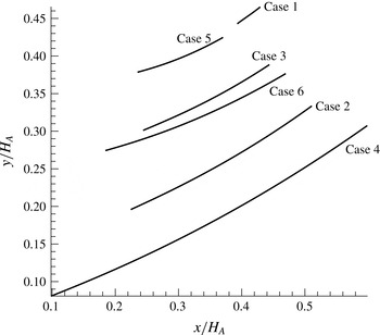
Figure 11. Shape of the reflected shock wave.

Figure 12. Shock angle of the reflected shock wave.
We have seen in table 2 that the error in the prediction of Mach stem height is relatively large for cases 5 and 6. When we look at table 3, we see that the slipline angle
 $\unicode[STIX]{x1D6FF}_{s}^{T}$
at the triple point is large for cases 5 and 6. In these cases, the secondary waves generated over the free part of the slipline are relatively strong so that the transmitted expansion waves should be more seriously disturbed by these secondary waves. This means that the utilization of regularized transmitted expansion waves rather than curved Mach waves would become less accurate for higher
$\unicode[STIX]{x1D6FF}_{s}^{T}$
at the triple point is large for cases 5 and 6. In these cases, the secondary waves generated over the free part of the slipline are relatively strong so that the transmitted expansion waves should be more seriously disturbed by these secondary waves. This means that the utilization of regularized transmitted expansion waves rather than curved Mach waves would become less accurate for higher
 $\unicode[STIX]{x1D6FF}_{s}^{T}$
. Gao & Wu (Reference Gao and Wu2010) used a point-wise wave interaction model so that the curvature of transmitted expansion waves can be captured. Thus for these two cases they gave better results (with an error of 3.2 % compared to 14.5 % by the present theory in case 5, and an error of 4.9 % compared to 13.3 % by the present theory in case 6). A future study to improve the accuracy of the present model would be the improvement of the regularized transmitted expansion wave model (for instance, by introducing a physically related model to make the transmitted expansion waves have a change of direction).
$\unicode[STIX]{x1D6FF}_{s}^{T}$
. Gao & Wu (Reference Gao and Wu2010) used a point-wise wave interaction model so that the curvature of transmitted expansion waves can be captured. Thus for these two cases they gave better results (with an error of 3.2 % compared to 14.5 % by the present theory in case 5, and an error of 4.9 % compared to 13.3 % by the present theory in case 6). A future study to improve the accuracy of the present model would be the improvement of the regularized transmitted expansion wave model (for instance, by introducing a physically related model to make the transmitted expansion waves have a change of direction).
3.3 Properties of the turning point of the slipline and significance
In § 3.2 a discontinuity of the slope of slipline at the turning point is found. As shown in figure 13, we use
 $\unicode[STIX]{x1D6FF}_{s}^{BL}$
to denote the slope at B on its left side, and
$\unicode[STIX]{x1D6FF}_{s}^{BL}$
to denote the slope at B on its left side, and
 $\unicode[STIX]{x1D6FF}_{s}^{BR}$
the slope at B on its right side. Table 4 shows
$\unicode[STIX]{x1D6FF}_{s}^{BR}$
the slope at B on its right side. Table 4 shows
 $\unicode[STIX]{x1D6FF}_{s}^{BL}$
,
$\unicode[STIX]{x1D6FF}_{s}^{BL}$
,
 $\unicode[STIX]{x1D6FF}_{s}^{BR}$
, the slope difference
$\unicode[STIX]{x1D6FF}_{s}^{BR}$
, the slope difference
 $\unicode[STIX]{x1D703}_{s}^{B}=\unicode[STIX]{x1D6FF}_{s}^{BL}-\unicode[STIX]{x1D6FF}_{s}^{BR}$
and the derivatives
$\unicode[STIX]{x1D703}_{s}^{B}=\unicode[STIX]{x1D6FF}_{s}^{BL}-\unicode[STIX]{x1D6FF}_{s}^{BR}$
and the derivatives
 $\text{d}\unicode[STIX]{x1D6FF}_{s}^{BL}/\text{d}x$
,
$\text{d}\unicode[STIX]{x1D6FF}_{s}^{BL}/\text{d}x$
,
 $\text{d}\unicode[STIX]{x1D6FF}_{s}^{BR}/\text{d}x$
at point B. The slope difference
$\text{d}\unicode[STIX]{x1D6FF}_{s}^{BR}/\text{d}x$
at point B. The slope difference
 $\unicode[STIX]{x1D703}_{s}^{B}$
is several degrees in all cases and is the largest for case 1. There is also a discontinuity of the derivative
$\unicode[STIX]{x1D703}_{s}^{B}$
is several degrees in all cases and is the largest for case 1. There is also a discontinuity of the derivative
 $\text{d}\unicode[STIX]{x1D6FF}_{s}^{BL}/\text{d}x-\text{d}\unicode[STIX]{x1D6FF}_{s}^{BR}/\text{d}x$
.
$\text{d}\unicode[STIX]{x1D6FF}_{s}^{BL}/\text{d}x-\text{d}\unicode[STIX]{x1D6FF}_{s}^{BR}/\text{d}x$
.

Figure 13. Turning point B.
The slope difference
 $\unicode[STIX]{x1D703}_{s}^{B}$
represents a flow deflection angle, and such a flow angle deviation should produce a shock wave if the slip line could be considered as a wall. However, a slipline cannot sustain a single oblique shock wave like a solid wall. Possibly, a series of compression waves (
$\unicode[STIX]{x1D703}_{s}^{B}$
represents a flow deflection angle, and such a flow angle deviation should produce a shock wave if the slip line could be considered as a wall. However, a slipline cannot sustain a single oblique shock wave like a solid wall. Possibly, a series of compression waves (
 $C_{t}$
) lie in the close vicinity of point B, as shown in figure 13, and these compression waves focus soon into a shock wave, which may be the wave
$C_{t}$
) lie in the close vicinity of point B, as shown in figure 13, and these compression waves focus soon into a shock wave, which may be the wave
 $\text{BB}^{\prime }$
shown in figure 3.
$\text{BB}^{\prime }$
shown in figure 3.
If
 $\text{BB}^{\prime }$
is a compression Mach wave, the direction of
$\text{BB}^{\prime }$
is a compression Mach wave, the direction of
 $\text{BB}^{\prime }$
is determined by the Mach angle
$\text{BB}^{\prime }$
is determined by the Mach angle
 $\unicode[STIX]{x1D707}_{B}=\arcsin (1/Ma_{s}^{B})$
and the initial direction (direction of
$\unicode[STIX]{x1D707}_{B}=\arcsin (1/Ma_{s}^{B})$
and the initial direction (direction of
 $\text{BB}^{\prime }$
close to point B) with respect to the horizontal axis is
$\text{BB}^{\prime }$
close to point B) with respect to the horizontal axis is
 $\unicode[STIX]{x1D6FC}_{\unicode[STIX]{x1D707}}^{B}=\unicode[STIX]{x1D707}_{B}-\unicode[STIX]{x1D6FF}_{s}^{BL}$
. If it is a shock wave, this direction is determined by
$\unicode[STIX]{x1D6FC}_{\unicode[STIX]{x1D707}}^{B}=\unicode[STIX]{x1D707}_{B}-\unicode[STIX]{x1D6FF}_{s}^{BL}$
. If it is a shock wave, this direction is determined by
 $\unicode[STIX]{x1D6FC}_{\unicode[STIX]{x1D6FD}}^{B}=\unicode[STIX]{x1D6FD}_{B}-\unicode[STIX]{x1D6FF}_{s}^{BL}$
, where
$\unicode[STIX]{x1D6FC}_{\unicode[STIX]{x1D6FD}}^{B}=\unicode[STIX]{x1D6FD}_{B}-\unicode[STIX]{x1D6FF}_{s}^{BL}$
, where
 $\unicode[STIX]{x1D6FD}_{B}$
is the shock angle of a hypothetical shock wave that would be produced at point B if the flow direction deviates an angle
$\unicode[STIX]{x1D6FD}_{B}$
is the shock angle of a hypothetical shock wave that would be produced at point B if the flow direction deviates an angle
 $\unicode[STIX]{x1D703}_{s}^{B}$
.
$\unicode[STIX]{x1D703}_{s}^{B}$
.

Figure 14. Hypothetical shock wave and Mach wave superimposed on the CFD contour lines, taken respectively from Ben-Dor et al. (Reference Ben-Dor, Ivanov, Vasilev and Elperin2002) and Gao & Wu (Reference Gao and Wu2010).
Table 4. Some parameters at the turning point B.
Table 5 displays the results for several conditions with CFD results. The direction
 $\unicode[STIX]{x1D6FC}_{cfd}^{B}$
is measured from the CFD contourlines, with the first two cases given by Gao & Wu (Reference Gao and Wu2010) and the last three cases given by Ben-Dor et al. (Reference Ben-Dor, Ivanov, Vasilev and Elperin2002). We draw a line
$\unicode[STIX]{x1D6FC}_{cfd}^{B}$
is measured from the CFD contourlines, with the first two cases given by Gao & Wu (Reference Gao and Wu2010) and the last three cases given by Ben-Dor et al. (Reference Ben-Dor, Ivanov, Vasilev and Elperin2002). We draw a line
 $\text{BB}^{\prime }$
which coincides with the slope change line of contourlines and
$\text{BB}^{\prime }$
which coincides with the slope change line of contourlines and
 $\unicode[STIX]{x1D6FC}_{cfd}^{B}$
is the direction of
$\unicode[STIX]{x1D6FC}_{cfd}^{B}$
is the direction of
 $\text{BB}^{\prime }$
approaching the point B. There is of course some uncertainty for measuring
$\text{BB}^{\prime }$
approaching the point B. There is of course some uncertainty for measuring
 $\unicode[STIX]{x1D6FC}_{cfd}^{B}$
in this way. It is seen that the measured value
$\unicode[STIX]{x1D6FC}_{cfd}^{B}$
in this way. It is seen that the measured value
 $\unicode[STIX]{x1D6FC}_{cfd}^{B}$
is more close to the shock solution (
$\unicode[STIX]{x1D6FC}_{cfd}^{B}$
is more close to the shock solution (
 $\unicode[STIX]{x1D6FC}_{\unicode[STIX]{x1D6FD}}^{B}$
) than the Mach wave solution (
$\unicode[STIX]{x1D6FC}_{\unicode[STIX]{x1D6FD}}^{B}$
) than the Mach wave solution (
 $\unicode[STIX]{x1D6FC}_{\unicode[STIX]{x1D707}}^{B}$
) for all the five cases. This would suggest that the slope discontinuity at the turning point B produces a weak shock wave. Figure 14 displays the slope change line of contours, hypothetical shock wave from point B and hypothetical Mach wave from point B, for one case by Gao & Wu (Reference Gao and Wu2010) and one case by Ben-Dor et al. (Reference Ben-Dor, Ivanov, Vasilev and Elperin2002) (which comes from Ivanov et al.
Reference Ivanov, Ben-Dor, Elperin, Kudryavtsev and Khotyanovsky2001). The difference in the direction of the hypothetical shock wave and hypothetical Mach wave are not as pronounced in figure 14 as in table 5. One may draw the conclusion that, close to the point B, the line with change of slope of contours is better approached by the hypothetical shock wave from point B, generated due to a flow deflection angle
$\unicode[STIX]{x1D6FC}_{\unicode[STIX]{x1D707}}^{B}$
) for all the five cases. This would suggest that the slope discontinuity at the turning point B produces a weak shock wave. Figure 14 displays the slope change line of contours, hypothetical shock wave from point B and hypothetical Mach wave from point B, for one case by Gao & Wu (Reference Gao and Wu2010) and one case by Ben-Dor et al. (Reference Ben-Dor, Ivanov, Vasilev and Elperin2002) (which comes from Ivanov et al.
Reference Ivanov, Ben-Dor, Elperin, Kudryavtsev and Khotyanovsky2001). The difference in the direction of the hypothetical shock wave and hypothetical Mach wave are not as pronounced in figure 14 as in table 5. One may draw the conclusion that, close to the point B, the line with change of slope of contours is better approached by the hypothetical shock wave from point B, generated due to a flow deflection angle
 $\unicode[STIX]{x1D703}_{s}^{B}$
.
$\unicode[STIX]{x1D703}_{s}^{B}$
.

Figure 15. Dividing point
 $q$
from which the Mach wave intersects point F.
$q$
from which the Mach wave intersects point F.
Table 5. Shock angle and Mach angle and directions of hypothetical shock wave or Mach wave
 $\text{BB}^{\prime }$
produced by the turning point. Here
$\text{BB}^{\prime }$
produced by the turning point. Here
 $\unicode[STIX]{x1D6FC}_{\unicode[STIX]{x1D6FD}}^{B}=\unicode[STIX]{x1D6FD}_{B}-\unicode[STIX]{x1D6FF}_{s}^{BL}$
and
$\unicode[STIX]{x1D6FC}_{\unicode[STIX]{x1D6FD}}^{B}=\unicode[STIX]{x1D6FD}_{B}-\unicode[STIX]{x1D6FF}_{s}^{BL}$
and
 $\unicode[STIX]{x1D6FC}_{\unicode[STIX]{x1D707}}^{B}=\unicode[STIX]{x1D707}_{B}-\unicode[STIX]{x1D6FF}_{s}^{BL}$
.
$\unicode[STIX]{x1D6FC}_{\unicode[STIX]{x1D707}}^{B}=\unicode[STIX]{x1D707}_{B}-\unicode[STIX]{x1D6FF}_{s}^{BL}$
.
As shown in figure 15, there is a dividing point, denoted
 $q$
, on the free part of the slipline, the Mach wave coming from this point intersects point F. The position of
$q$
, on the free part of the slipline, the Mach wave coming from this point intersects point F. The position of
 $q$
is thus given by
$q$
is thus given by
 $$\begin{eqnarray}y_{F}-y_{q}=(x_{F}-x_{q})\tan (\unicode[STIX]{x1D707}_{s}^{+}-\unicode[STIX]{x1D6FF}_{s}),\end{eqnarray}$$
where
 $\unicode[STIX]{x1D707}_{s}^{+}=\arcsin (1/M_{s}^{+})$
is the Mach angle. Table 6 displays the position and slope at this point. Hence, the difference of slopes between point
$\unicode[STIX]{x1D707}_{s}^{+}=\arcsin (1/M_{s}^{+})$
is the Mach angle. Table 6 displays the position and slope at this point. Hence, the difference of slopes between point
 $q$
and the triple point,
$q$
and the triple point,
 $\unicode[STIX]{x1D6FF}_{s}^{q}-\unicode[STIX]{x1D6FF}_{s}^{T}$
is one order smaller than
$\unicode[STIX]{x1D6FF}_{s}^{q}-\unicode[STIX]{x1D6FF}_{s}^{T}$
is one order smaller than
 $\unicode[STIX]{x1D6FF}_{s}^{BL}-\unicode[STIX]{x1D6FF}_{s}^{T}$
(the difference of slopes between point B and point T). This means that the expansion waves generated on the free part of the slipline have little influence on the head part TF of the reflected shock wave.
$\unicode[STIX]{x1D6FF}_{s}^{BL}-\unicode[STIX]{x1D6FF}_{s}^{T}$
(the difference of slopes between point B and point T). This means that the expansion waves generated on the free part of the slipline have little influence on the head part TF of the reflected shock wave.
Expansion waves generated over the segment
 $q\text{B}$
of the slipline enters into the region of transmitted expansion waves. This shall disturb the transmitted expansion waves. However, the hypothetical weak shock
$q\text{B}$
of the slipline enters into the region of transmitted expansion waves. This shall disturb the transmitted expansion waves. However, the hypothetical weak shock
 $\text{BB}^{\prime }$
has a counter effect to cancel the overall effect of this perturbation. According to the last column of table 6, the slope
$\text{BB}^{\prime }$
has a counter effect to cancel the overall effect of this perturbation. According to the last column of table 6, the slope
 $\unicode[STIX]{x1D6FF}_{s}^{BR}$
is almost equal to
$\unicode[STIX]{x1D6FF}_{s}^{BR}$
is almost equal to
 $\unicode[STIX]{x1D6FF}_{s}^{T}$
, hence the total amount of expansion (over
$\unicode[STIX]{x1D6FF}_{s}^{T}$
, hence the total amount of expansion (over
 $q\text{B}$
) and compression (by
$q\text{B}$
) and compression (by
 $\text{BB}^{\prime }$
at point B) almost cancels out. This may be the reason that the regularized transmitted expansion wave assumption adopted here works.
$\text{BB}^{\prime }$
at point B) almost cancels out. This may be the reason that the regularized transmitted expansion wave assumption adopted here works.
Table 6. Parameters near the dividing point
 $q$
, compared to the turning point B.
$q$
, compared to the turning point B.
4 Concluding remarks
In this paper analytical expressions for the slipline and reflected shock wave for Mach reflection in steady supersonic flow are derived. The effect of secondary expansion waves or compression waves over the slipline is included in the theory. The transmitted expansion waves, which should be curved due to the interaction of these secondary waves, are treated as straight lines (assumption of regularized transmitted expansion waves) in this paper. An easily solvable algorithm is provided that gives simultaneously the Mach stem height and the shape of slipline and reflected shock wave.
Due to the analytical treatment of the slipline, the turning point of the slipline can be studied in detail, this point is the intersection of the slipline with the leading characteristics of the expansion wave from the wedge corner. By this study, a slope discontinuity, of several degrees for the conditions considered in this paper, is discovered.
When using this slope discontinuity as the flow deflection angle, the calculated hypothetical shock wave matches an apparent wave seen from CFD results. Across this apparent wave, the contour lines of flow parameters change direction abruptly. The slope discontinuity of the slipline at the turning point and the existence of a hypothetical shock wave are new findings of this paper.
Thus, Mach reflection in steady supersonic flow contains an additional shock wave arising from the turning point of the slipline, though this shock wave may be very weak depending on the flow conditions.
The secondary expansion waves produced over the slipline have one part intersecting the front portion of the reflected shock wave and another part intersecting directly the transmitted expansion waves. It is found that the strength of the first part is negligible while the second part can not be neglected. This means that the front part of the reflected shock wave can be regarded as a straight shock wave. However, the second part corresponds to a total deflection angle that is almost equal to the negative of the slope discontinuity at the turning point. This means that the total effect by these secondary expansion waves almost cancel out the effect of the compression wave from the turning point. As a result, the transmitted expansion waves carry the information from the reflected shock wave to the slipline as if they were straight characteristics. This is the reason to have a simple and fast model for prediction of the Mach stem height and shapes of slipline and reflected shock wave, and the accuracy is very good if the slope of the slipline at the triple point is a few degrees. The predicted Mach stem height compares very well with the recent experimental data and CFD data for small shock angles, for the case with
 $H_{R}/w=0.4$
and
$H_{R}/w=0.4$
and
 $M_{0}=3.98$
.
$M_{0}=3.98$
.
Utilization of the regularized transmitted expansion wave assumption causes a relatively large error in the estimation of the Mach stem height for large slipline angle at the triple point. Thus, if the accuracy of the model should be improved, a better (but simpler than the point-wise wave interaction model of Gao & Wu Reference Gao and Wu2010) treatment of the transmitted expansion waves needs to be studied.
Acknowledgements
We are grateful to the referees for their valuable comments that helped to clarify a number of questions and to improve the paper. This work was supported by the Natural National Science Foundation of China (no. 11472157).


