3.1. Uniform momentum zones

The dynamics within the UMZs is governed by the two-dimensional (2-D) but three-component (i.e. $x$-independent) NS equations, since the streamwise-varying fluctuation fields are exponentially small. Thus, the momentum equations reduce to

(3.2)\begin{gather} \partial_t \bar{u}+\left( \bar{\boldsymbol{v}}_{\bot}\boldsymbol{\cdot}\boldsymbol{\nabla}_\bot \right)\bar{u}=\frac{1}{Re}\nabla_\bot^2\bar{u}, \end{gather}

(3.3)\begin{gather}\partial_t \bar{\boldsymbol{v}}_{\bot} + \left(\bar{\boldsymbol{v}}_{\bot}\boldsymbol{\cdot}\boldsymbol{\nabla}_\bot\right) \bar{\boldsymbol{v}}_{\bot}=-\boldsymbol{\nabla}_\bot \bar{p}+\frac{1}{Re}\nabla_\bot^2\bar{\boldsymbol{v}}_{\bot}, \end{gather}

where the $\bot$ subscript refers to the $y$–$z$ plane and the perpendicular (i.e. roll) velocity vector $\bar {\boldsymbol {v}}_\bot =(\bar {v},\bar {w})$. From (3.2), it is clear that the mean streamwise velocity acts as a passive scalar within the UMZs, being advected by the rolls and diffused. The rolls are not directly forced within the UMZs and therefore would decay in the absence of the forcing localized within the bounding VFs. An immediate and significant physical implication is that the internal layers (sometimes referred to as ‘interfaces’ in the literature, e.g. see de Silva et al. Reference de Silva, Philip, Hutchins and Marusic2017) are not dynamically passive; rather, the driving agency for the staircase-like profiles of streamwise velocity is confined within the regions of concentrated vorticity.

As noted in § 2, we insist that the dynamical influence of viscosity on the streak and roll flow is weak, at least in a volume-averaged sense. In particular, if the amplitude of the roll flow is denoted by $\bar {a}$, where $\bar {a}(Re)\to 0$ as $Re\to \infty$ (implying that the rolls are weak compared to the $\mathit {O}(1)$ streamwise streak flow), then we require the effective Reynolds number $\bar {a}Re$ governing the dynamics of the rolls and streaks within the UMZs to become unbounded in the large-$Re$ limit. It is well known that in the presence of a steady cellular (2-D) velocity field, a passive scalar will be homogenized in the limit of large Péclet number (Rhines & Young Reference Rhines and Young1983). Since $\bar {a}Re\to \infty$, and given that we seek stacked ECS with steady rolls, the passive streak velocity field $\bar {u}$ therefore is differentially homogenized within regions of closed streamlines of the roll flow.

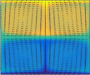
This process is clearly depicted in figure 6. The right-hand plot shows the initial and steady-state spanwise-averaged streamwise velocity profiles $\overline {u}^{xz}(y)$. These profiles are obtained by numerically integrating (3.2) using a Fourier–Chebyshev pseudospectral algorithm with the prescribed steady roll velocity field given below in (3.9)–(3.10) and plotted in figure 6(a) for an effective Reynolds number $\bar {a}Re\approx 10^4$. Of particular note is the emergence of an internal shear layer centred on the plane $y=0$.

Figure 6. Differential homogenization of a background Couette flow (a,b) by stacked, counter-rotating steady rolls (vector plot in (a), obtained from (3.9)–(3.10)) leading to the emergence of UMZs and an internal shear layer (b); i.e. an embedded VF. This process is realized only for sufficiently large values of the effective Reynolds number $\bar {a}Re$, where the roll amplitude $\bar {a}(Re)\to 0$ as $Re\to \infty$. For example, in the Fourier–Chebyshev pseudospectral computations used to generate these results, $\bar {a}Re\approx 10^4$ (and $\bar {\Omega }_c\approx 7.35$.)

Rhines & Young (Reference Rhines and Young1983) demonstrate that if the evolution is laminar (e.g. driven by a strictly steady 2-D cellular velocity field acting on a scalar field exhibiting a uniform gradient at some initial time, say $t=0$), scalar homogenization in the large Péclet number ($Pe$) limit generically occurs in two stages. During a time $t=\mathit {O}(Pe^{1/3})$, shear-augmented dispersion acts to homogenize the scalar field along streamlines. The subsequent homogenization of the scalar field across streamlines occurs over a much longer time $t=\mathit {O}(Pe)$. Crucially, diffusion is a leading-order process only during the first phase: in the present context, advection dominates perturbations due to diffusion, ‘locking’ contours of constant $\bar {u}$ to the streamline pattern induced by the rolls, throughout the second phase as well as in the final steady state. Plausibly, the time scale for homogenization may be reduced by turbulent mixing processes, but we make no judgment regarding the time taken for a turbulent trajectory to visit the neighbourhood of the steady ECS we construct. Nevertheless, we emphasize that within the UMZs viscous diffusion is a weak dynamical process relative to roll-induced advection for these ECS, in accord with the mean momentum balance outboard of the Reynolds stress peak (figure 2a).

For steady rolls and streaks within the homogenized core of the UMZs, the following asymptotic expansions are posited:

(3.4)\begin{gather} u(x,y,z,t;Re)\sim \overline{u}_0(y,z)+\mbox{E.S.T.}, \end{gather}

(3.5)\begin{gather}v(x,y,z,t;Re)\sim \bar{a}\overline{v}_2(y,z)+\cdots, \end{gather}

(3.6)\begin{gather}w(x,y,z,t;Re)\sim \bar{a}\overline{w}_2(y,z)+\cdots, \end{gather}

(3.7)\begin{gather}p(x,y,z,t;Re)\sim \bar{a}^2\overline{p}_4(y,z)+\cdots. \end{gather}

The numeric subscripts refer to a posteriori determined powers of the small parameter $\Delta$ defining $\bar {a}$, and E.S.T. denotes terms that are exponentially small in $Re$. These terms include the $x$-varying fluctuation fields within the UMZs and transcendentally small corrections to the homogenized fields. Indeed, not only is $\bar {u}$ homogenized but, in accord with the Prandtl–Batchelor theorem (Batchelor Reference Batchelor1956), the steady $x$-mean $x$-vorticity $\bar {\Omega }$ also is uniform within regions foliated by steady closed streamlines on which viscous diffusion is weak relative to advection. That is,

(3.8)\begin{equation} \bar{\Omega}\equiv\partial_y\bar{w}-\partial_z\bar{v}\sim \nabla_\bot^2\left(\bar{a}\overline{\psi}_2\right)\sim\bar{a}\bar{\Omega}_c + \mbox{E.S.T.},\end{equation}

where the (rescaled) roll streamfunction $\overline {\psi }_2(y,z)$ is defined by $(\kern .5pt\overline {v}_2,\overline {w}_2)=(-\partial _z\overline {\psi }_2,\partial _y\overline {\psi }_2)$. Unlike the constant core value of the $x$-mean streamwise velocity, which by symmetry must satisfy $\overline {u}_0\sim 1/2$ for $0<y<1$ and $\overline {u}_0=-1/2$ for $-1<y<0$, the (rescaled) homogenized value of the $x$-mean $x$-vorticity $\bar {\Omega }_c$, which fixes the precise value of the roll-induced circulation, is a primary unknown to be determined as part of the asymptotic analysis: effectively, $\bar {\Omega }_c$ is a nonlinear eigenvalue that will be shown to couple information from the various subdomains of the flow. Nonetheless, as demonstrated in Chini (Reference Chini2008), (3.8) is readily solved analytically on a rectangular domain of (asymptotically) known dimensions one unit in $y$ and $L_z/2$ units in $z$ (where $L_z$ is the prescribed spanwise periodicity length of the rolls), subject to $\overline {\psi }_2(y,z)\to 0$ as the rectangular cell boundaries are approached. Using the given notation,

(3.9)\begin{gather} \overline{v}_{2} = \bar{\Omega}_c\sum_{n=1, \mathrm{odd}}^{\infty}\frac{2L_z}{(n{\rm \pi})^2}\left[\frac{\cosh[(2n{\rm \pi}/ L_z)(1/2-y)]}{\cosh(n{\rm \pi}/L_z)}-1\right]\cos{\left(\frac{2n{\rm \pi} z}{L_z}\right)}, \end{gather}

(3.10)\begin{gather}\overline{w}_{2} =\bar{\Omega}_c\sum_{n=1, \mathrm{odd}}^{\infty}\frac{2L_z}{(n{\rm \pi})^2}\left[\frac{\sinh[(2n{\rm \pi}/L_z)(1/2-y)]}{\cosh(n{\rm \pi}/L_z)}\right] \sin{\left(\frac{2n{\rm \pi} z}{L_z}\right)}. \end{gather}

To avoid the need for iteration in the subsequent solution algorithm, and noting that $\bar {\Omega }_c = O(1)$, it proves useful here to introduce the slightly modified small parameter $\tilde {\Delta } = \bar {\Omega }_c^{-1/4}\Delta$ and rescaled mean fields $\bar {v} = \bar {\Omega }_c\tilde {v}$, $\bar {w} = \bar {\Omega }_c\tilde {w}$ and $\bar {p} = \bar {\Omega }_c^2\tilde {p}$, where all fields are (re-)expanded in asymptotic series in powers of $\tilde {\Delta }$ rather than $\Delta$. With this rescaling the governing equations in the UMZ become

(3.11)\begin{gather} \left( \tilde{\boldsymbol{v}}_{2\bot}\boldsymbol{\cdot}\boldsymbol{\nabla}_\bot \right)\bar{u}_{0}= \tilde{\Delta}^2\nabla_\bot^2\overline{u}_{0}, \end{gather}

(3.12)\begin{gather}\left(\tilde{\boldsymbol{v}}_{2\bot}\boldsymbol{\cdot}\boldsymbol{\nabla}_\bot\right)\tilde{\boldsymbol{v}}_{2\bot}=-\boldsymbol{\nabla}_\bot \tilde{p}_{4}+\tilde{\Delta}^2\nabla_\bot^2\tilde{\boldsymbol{v}}_{2\bot}. \end{gather}

Thus, with the understanding that $\bar {\Omega }_c$ is a to-be-determined constant, the steady roll velocity field within the UMZs is known, a key simplification.

3.2. Vortical fissures

In the asymptotic limit $Re\to \infty$, the differential homogenization of $\bar {\Omega }$ leads to jump discontinuities in this field across the separatrices between adjacent roll cells. Moreover, in addition to the jumps in $\bar {u}$ induced between stacked cells, streamwise velocity anomalies in the form of narrow jets are driven between neighbouring roll pairs at each fixed $y$ location away from the fissures. These various discontinuities are smoothed by viscous forces and torques that act on the mean fields within asymptotically thin regions along the periphery of each cell. Here, we focus on the emergent shear layer centred on $y=0$, but analogous considerations apply to all other VFs (located at $y=n$, for integer $n=\pm 1, \pm 2\ldots$). Similar scalings also apply to the narrow jets centred on $z=m L_z/2$, for integer $m=0, \pm 1, \pm 2\ldots$, albeit with the roles of $y$ and $z$ interchanged and with the important distinction that, unlike the VFs, the jets are dynamically passive since in the present theory the $x$-varying fluctuations are exponentially small there.

The thickness of each VF follows from the usual laminar-BL scaling in which normal diffusion is balanced with advection, viz. $\tilde {\Delta }=(\bar {a}\bar {\Omega }_c Re)^{-1/2}$. For the VF centred on $y=0$, we therefore introduce a rescaled $y$ coordinate ${\mathcal {Y}}\equiv y/\tilde {\Delta }$, and we decompose all field variables into mean plus slowly modulated fluctuation components:

(3.13)\begin{align} \begin{bmatrix} u(x,y,z,t;Re)\\ v(x,y,z,t;Re)\\ w(x,y,z,t;Re)\\ p(x,y,z,t;Re) \end{bmatrix} &\sim \begin{bmatrix} \overline{{\mathcal{U}}}_0({\mathcal{Y}},z)\\ \bar{a}\tilde{\Delta}\overline{{\mathcal{V}}}_3({\mathcal{Y}},z)\\ \bar{a}\,\overline{{\mathcal{W}}}_2({\mathcal{Y}},z)\\ \bar{a}^2\overline{{\mathcal{P}}}_4({\mathcal{Y}},z) \end{bmatrix} \nonumber\\ &\quad +a'{\mathcal{A}} \begin{bmatrix} \hat{{\mathcal{U}}}_3({\mathcal{Y}};z)\\ \hat{{\mathcal{V}}}_3({\mathcal{Y}};z)\\ \hat{{\mathcal{W}}}_3({\mathcal{Y}};z)\\ \hat{{\mathcal{P}}}_3({\mathcal{Y}};z) \end{bmatrix} A(z)\exp\left({\textrm{i}\big[\alpha (x-ct)+\theta(z/\tilde{\Delta})\big]}\right)+\textrm{c.c.}, \end{align}

where c.c. denotes complex conjugate. In these expansions, the fluctuations, which have a to-be-determined asymptotic magnitude $a'(Re)$ and $\mathit {O}(1)$$z$-varying amplitude ${\mathcal {A}}A(z)$, are represented using a WKBJ approximation in which the fast phase $\theta (z/\tilde {\Delta })\equiv \Theta (z)/\tilde {\Delta }$ and the rescaled spanwise wavenumber $\tilde {\beta }\equiv \partial _z\Theta =\mathit {O}(1)$. We also define the $O(1)$ streamwise wavenumber $\tilde {\alpha } = \alpha \tilde {\Delta }$ and, for subsequent reference, note that $\breve {\alpha } = \tilde {\alpha }\bar {\Omega }_c^{1/4}$, i.e. the $O(1)$ streamwise wavenumber scaled by $\Delta$ rather than by $\tilde {\Delta }$. The $\mathit {O}(1)$ phase speed $c$ is strictly real for neutral Rayleigh modes implicated in a steady SSP and vanishes only for the VF at $y=0$. Although the real scalar ${\mathcal {A}}$ could be absorbed into the definition of the amplitude function $A(z)$, it proves convenient to explicitly retain this factor as a control parameter. (That is, we take ${\mathcal {A}}$ and the rescaled, $\mathit {O}(1)$ streamwise wavenumber $\breve {\alpha }$ as control parameters for the Rayleigh mode and self-consistently determine the slowly varying spanwise wavenumber $\tilde {\beta }(z)$ and amplitude function $A(z)$.) To disentangle ${\mathcal {A}}$ from $A(z)$, we normalize the latter such that $A(0)=1$. An additional normalization condition will be specified below to distinguish the ${\mathcal {Y}}$- and $z$-varying eigenfunction from the amplitude, thereby rendering the decomposition of the fluctuation fields in (3.13) unique.

The scaling of the mean streamwise and spanwise velocity components in (3.13) ensures smooth matching with the flow in the adjacent UMZs is possible, while the scaling of the mean fissure-normal velocity follows from incompressibility. In the proposed configuration, no physical (i.e. no-slip) boundary exists along the horizontal planes separating rows of stacked counter-rotating rolls. Consequently, the leading-order mean spanwise velocity component within the VF is not sheared; i.e. $\partial _{{\mathcal {Y}}}\overline {{\mathcal {W}}}_2=0$, hence $\overline {{\mathcal {W}}}_2=\overline {{\mathcal {W}}}_2(z)$, only. Through the mean incompressibility condition, this ansatz implies that within the fissure $\overline {{\mathcal {V}}}_3({\mathcal {Y}},z)$ varies linearly with the normal coordinate ${\mathcal {Y}}$. A second immediate consequence is that the roll vorticity will have the same asymptotic size, namely $\mathit {O}(\bar {a})$, within the VF and adjacent UMZs, ensuring smooth matching of this field is possible. To close the global vorticity budget, however, a ${\mathcal {Y}}$-dependent correction $\bar {a}\tilde {\Delta }\overline {{\mathcal {W}}}_3({\mathcal {Y}},z)$ must be appended to the expansion for the mean spanwise velocity component in (3.13); see Harper (Reference Harper1963). Finally, in contrast to the mean fields, the fluctuations are isotropic within the fissure and thus each fluctuation field has the same asymptotic magnitude $a'$. (We find that $a'\le \bar {a}$ as $Re\to \infty$ for sensible physical balances to be realized in the mean equations.) Recalling that the streamwise wavelength of the fluctuation fields is commensurate with ${\Delta }$, the VF thickness, the fluctuations consequently decay exponentially away from the centre of the fissure.

3.2.1. Viscous mean dynamics: Childress cell problem

Substituting (3.13) into the incompressibility condition and the NS equations, applying the streamwise/fast-phase averaging operation and collecting terms at leading order in $\tilde {\Delta }$ yields

(3.14)\begin{gather} \partial_{{\mathcal{Y}}}\tilde{{\mathcal{V}}}_3+\partial_z\tilde{{\mathcal{W}}_2}=0, \end{gather}

(3.15)\begin{gather}\tilde{{\mathcal{V}}}_3\partial_{{{\mathcal{Y}}}}\overline{{\mathcal{U}}}_0+\tilde{{\mathcal{W}}}_2\partial_z\overline{{\mathcal{U}}}_0= \partial_{{{\mathcal{Y}}}}^2\overline{{\mathcal{U}}}_0, \end{gather}

(3.16)\begin{gather}\partial_{{\mathcal{Y}}}\tilde{{\mathcal{P}}}_4=0, \end{gather}

(3.17)\begin{gather}\tilde{{\mathcal{W}}}_2\partial_z\tilde{{\mathcal{W}}}_2=-\partial_z\tilde{{\mathcal{P}}}_4, \end{gather}

(3.18)\begin{gather}\tilde{{\mathcal{V}}}_3\partial_{{{\mathcal{Y}}}}\left(\partial_{{\mathcal{Y}}}\tilde{{\mathcal{W}}}_3\right)+\tilde{{\mathcal{W}}}_2\partial_z\left(\partial_{{\mathcal{Y}}}\tilde{{\mathcal{W}}}_3\right)=-\frac{\partial_{{\mathcal{Y}}}^2\left(\overline{{\mathcal{V}}'_3{\mathcal{W}}'_3}\right)}{\bar{\Omega}_c^2}+\partial_{{{\mathcal{Y}}}}^2\left(\partial_{{\mathcal{Y}}}\tilde{{\mathcal{W}}}_3\right), \end{gather}

where $(\overline {{\mathcal {V}}}_3,\overline {{\mathcal {W}}}_{2,3}) = \bar {\Omega }_c(\tilde {{\mathcal {V}}}_3,\tilde {{\mathcal {W}}}_{2,3})$ and $\overline {{\mathcal {P}}}_4=\bar {\Omega }_c^2\tilde {{\mathcal {P}}}_4$. The key simplification to the mean-flow equations in this region is that asymptotic matching enables the leading-order roll flow $(\tilde {{\mathcal {V}}}_3,\tilde {{\mathcal {W}}}_2)$ to be obtained by extrapolating the UMZ roll solution to the VF. Specifically, the tangential component of the roll flow in the fissure is obtained simply by evaluating (3.10) at $y = 0$. Using the incompressibility constraint (3.14) and the symmetry condition $\tilde {{\mathcal {V}}}_3({\mathcal {Y}} = 0,z) = 0$ to determine a constant of integration, the normal flow component $\tilde {{\mathcal {V}}}_3$ also can be determined, yielding

(3.19)\begin{gather} \tilde{{\mathcal{V}}}_{3}({{\mathcal{Y}}},z) = -{{\mathcal{Y}}} \sum_{n=1, \mathrm{odd}}^{\infty}\left(\frac{4}{n{\rm \pi}}\right)\tanh\left(\frac{n{\rm \pi}}{L_z}\right)\cos\left(\frac{2n{\rm \pi} z}{L_z}\right), \end{gather}

(3.20)\begin{gather}\tilde{w}_{2}(y=0,z) = \tilde{{\mathcal{W}}}_2(z) = \sum_{n=1, \mathrm{odd}}^{\infty}\left(\frac{2L_z}{(n{\rm \pi})^2}\right)\tanh\left(\frac{n{\rm \pi}}{L_z}\right)\sin\left(\frac{2n{\rm \pi} z}{L_z}\right). \end{gather}

The leading-order roll flow within the VF (3.19)–(3.20) satisfies the mean equations (3.14), (3.16) and (3.17), with $\tilde {{\mathcal {P}}}_4(z) = \tilde {p}_4(y$=$0,z)$ for matching with the adjacent UMZs.

Given (3.19) and (3.20), the ($\perp$) velocity field that advects the leading-order streak flow $(\overline {{\mathcal {U}}}_0)$ and $x$-vorticity $(\partial _{{\mathcal {Y}}}\tilde {{\mathcal {W}}}_3)$ within the fissure is known, and the equations for these fields effectively linearize. Analogous considerations apply to the viscous jet regions around the remainder of the roll-cell periphery. By choosing $a' = \tilde {\Delta }\overline {a}$, the torque provided by the gradient of the fluctuation-induced Reynolds stress divergence $-\partial _{{\mathcal {Y}}}(\overline {{\mathcal {V}}_3'{\mathcal {W}}_3'})$ arises consistently in (3.18) and seemingly has the potential to generate $x$-vorticity within the VF and, thence, to drive roll motions within the UMZ. Subsequently, however, it is confirmed that ${\mathcal {V}}_3'$ and ${\mathcal {W}}_3'$ are out of phase for a (3-D) neutral Rayleigh mode. Consequently, this correlation vanishes and no driving of the rolls by this mechanism is realized. Instead, as in VWI theory, the driving to sustain the roll motions arises from a critical-layer phenomenon (see §§ 3.3 and 3.4).

The vorticity equation (3.18) must be solved subject to the matching condition $\partial _{{\mathcal {Y}}}\tilde {{\mathcal {W}}}_3\rightarrow -1$ as ${\mathcal {Y}}\rightarrow \infty$ (e.g. for matching with the upper UMZ in $0\le z\le L_z/2$). The appropriate boundary condition on this vorticity component as ${\mathcal {Y}}\rightarrow 0^+$ is not obvious a priori, but will be determined in § 3.3. Indeed, in the absence of driving from the Reynolds stress term in (3.18), this boundary condition will be shown to give rise to the forcing that sustains the rolls, revealing that the CL plays a key role in maintaining the staircase-like profile of streamwise velocity in the proposed asymptotic SSP.

The mean streamwise momentum equation (3.15) must be solved subject to the symmetry conditions $\overline {{\mathcal {U}}}_0 \rightarrow 1/2$ as ${\mathcal {Y}}\rightarrow \infty$ (for the UMZ located in $0<y<1$) and $\overline {{\mathcal {U}}}_0 \rightarrow 0$ as ${\mathcal {Y}}\rightarrow 0$. Identical equations and boundary conditions apply within the VF centred on $y=1$ upon replacing $\tilde {\Delta }{\mathcal {Y}} \rightarrow 1-\tilde {\Delta }{\mathcal {Y}}$ and $z \rightarrow L_z/2-z$. The same steady advection–diffusion equation also applies within the streamwise jets centred on $z=0$ and $z = L_z/2$, with the roles of $y$ and $z$ (and $\tilde {{\mathcal {V}}}_3$ and $\tilde {{\mathcal {W}}}_2$) interchanged. The resulting problem for $\overline {{\mathcal {U}}}_0$ is formally identical to that for the temperature field in steady 2-D Rayleigh–Bénard convection (RBC) in the limit of asymptotically large Rayleigh number. This observation provides an interesting and potentially useful connection between coherent structures arising in strongly nonlinear convection and wall-bounded shear flows. (Of course, in RBC, the cellular flow is driven by buoyancy torques acting within vertical plumes, while in the proposed SSP, the roll flow is driven by Reynolds stresses arising from the nonlinear interaction of a streamwise-varying shear instability mode confined to the horizontal fissures.) As demonstrated in Chini & Cox (Reference Chini and Cox2009), the advected and diffused scalar field can be determined by formulating a Childress cell problem (Childress Reference Childress1979), in which the fissures and jets (or thermal boundary layers and plumes in the RBC context) around each cell are stitched together to form a connected domain; see figure 7. Here, we simply lift the key results from Chini & Cox (Reference Chini and Cox2009); see appendix A for further details. In particular, solution of the Childress cell problem yields the shear $\tilde {\lambda }(z) \equiv \partial _{{\mathcal {Y}}} \overline {{\mathcal {U}}}_0({\mathcal {Y}}=0,z)$ induced by the mean streamwise velocity component at the centre of the fissure.

Figure 7. Formulation of Childress cell problem, as adapted from Chini & Cox (Reference Chini and Cox2009). (a) Contour plot of $\overline {u}_0(y,z)$. (b) Corresponding multiregion asymptotic structure of a steady roll cell as $Re\to \infty$. The white region is the dynamically inviscid vortex core. The light grey regions indicate the $O(\Delta )$ thick VFs as well as $O(\Delta )$ thick positive and negative streamwise jets. The streamwise-averaged streamwise velocity is passively advected through the outer corner regions also indicated by the light grey shading. (The viscous inner corner regions highlighted in dark grey also are dynamically passive.) $\zeta$ is a stretched arc-length coordinate running around the cell perimeter, and $\eta$ is a scaled coordinate measuring distance normal to the VFs and jets.

The solution for $\tilde {\lambda }(z)$ obtained from the Childress cell problem, i.e. in the limit $Re\to\infty$, is compared in figure 8 to that obtained by numerically solving the advection–diffusion equation (3.11) for small but finite $\tilde {\Delta }^2$ (corresponding to large but finite $Re$). The two profiles agree closely except at $z=0$, where diffusion heals a passive singularity arising in the solution of the Childress cell problem. This validation enables the finite-$Re$ data (i.e. with viscous regularization) to be used in the calculation of the fluctuation velocities within the VF, which is considered next. This strategy proves to be more convenient and robust than attempting to directly reconstruct $\overline {{\mathcal {U}}}_0({\mathcal {Y}},z)$ from the solution of the Childress cell problem.

Figure 8. Normalized streak-induced shear $\tilde {\lambda }(z)\equiv \partial _{{\mathcal {Y}}}\overline {{\mathcal {U}}}_0(0,z)$ at the mid-plane of the VF obtained from the solution of the Childress cell problem (i.e. in the limit $Re\rightarrow \infty$, solid curve) and from the numerical solution of the full advection–diffusion equation (3.11) for finite $Re$ (dotted curve).

3.2.2. Inviscid fluctuation dynamics: Rayleigh, eikonal and amplitude equations

Recalling the WKBJ ansatz in (3.13), the leading-order equations for the fluctuation fields within the VF are

(3.21)\begin{gather} \textrm{i}\tilde{\alpha}\hat{{\mathcal{U}}}_3+\partial_{{\mathcal{Y}}}\hat{{\mathcal{V}}}_3+\textrm{i}\tilde{\beta}\hat{{\mathcal{W}}}_3=0, \end{gather}

(3.22)\begin{gather}\textrm{i}\tilde{\alpha}\left(\overline{{\mathcal{U}}}_0-c\right)\hat{{\mathcal{U}}}_3+\hat{{\mathcal{V}}}_3\partial_{{\mathcal{Y}}}\overline{{\mathcal{U}}}_0+\textrm{i}\tilde{\alpha}\hat{{\mathcal{P}}}_3=0, \end{gather}

(3.23)\begin{gather}\textrm{i}\tilde{\alpha}\left(\overline{{\mathcal{U}}}_0-c\right)\hat{{\mathcal{V}}}_3+\partial_{{\mathcal{Y}}}\hat{{\mathcal{P}}}_3=0, \end{gather}

(3.24)\begin{gather}\textrm{i}\tilde{\alpha}\left(\overline{{\mathcal{U}}}_0-c\right)\hat{{\mathcal{W}}}_3+\textrm{i}\tilde{\beta}\hat{{\mathcal{P}}}_3=0. \end{gather}

From (3.21)–(3.24), it can be deduced that $\hat {{\mathcal {V}}}_3$ and $\hat {{\mathcal {W}}}_3$ are ${\rm \pi} /2$ out of phase, confirming that the correlation $\overline {{\mathcal {V}}_3'{\mathcal {W}}_3'}=0$ in (3.18). Utilizing Squire's transformation, this 3-D system can be reduced to a 2-D system. Specifically, adding $\tilde {\alpha }\times$(3.22) to $\tilde {\beta }\times$(3.24) and dividing the sum by $\tilde {\alpha }$ yields

(3.25)\begin{gather} \textrm{i} \tilde{k} \hat{{\mathcal{U}}}_{3r}+\partial_{{\mathcal{Y}}}\hat{{\mathcal{V}}}_3=0, \end{gather}

(3.26)\begin{gather}\textrm{i}\tilde{k} \left(\overline{{\mathcal{U}}}_0-c\right)\hat{{\mathcal{U}}}_{3r}+\hat{{\mathcal{V}}}_3\partial_{{\mathcal{Y}}}\overline{{\mathcal{U}}}_0+\textrm{i} \tilde{k}\hat{\Pi}_3=0, \end{gather}

(3.27)\begin{gather}\textrm{i} \tilde{k} \left(\overline{{\mathcal{U}}}_0-c\right)\hat{{\mathcal{V}}}_3+\partial_{{\mathcal{Y}}}\hat{\Pi}_3=0, \end{gather}

along with a decoupled but important equation for $\hat {{\mathcal {W}}}_{3r}$,

(3.28)\begin{equation} \hat{{\mathcal{W}}}_{3r}= \frac{1}{\textrm{i}\tilde{k}}\frac{\tilde{\beta}}{\tilde{\alpha}}\frac{\hat{{\mathcal{V}}}_{3}\partial_{{\mathcal{Y}}}\overline{{\mathcal{U}}}_0}{(\overline{{\mathcal{U}}}_0-c)}, \end{equation}

where

(3.29)\begin{gather} \tilde{k}=\sqrt{\tilde{\alpha}^2+\tilde{\beta}^2},\quad \tilde{k}\hat{{\mathcal{P}}}_3=\tilde{\alpha}\hat{\Pi}_3, \end{gather}

(3.30)\begin{gather}\tilde{k}\hat{{\mathcal{U}}}_{3r}=\tilde{\alpha}\hat{{\mathcal{U}}}_3+\tilde{\beta}\hat{{\mathcal{W}}}_3\quad \Longleftrightarrow \quad \tilde{k}\hat{{\mathcal{U}}}_3=\tilde{\alpha}\hat{{\mathcal{U}}}_{3r}-\tilde{\beta}\hat{{\mathcal{W}}}_{3r}, \end{gather}

(3.31)\begin{gather}\tilde{k}\hat{{\mathcal{W}}}_{3r}=\tilde{\alpha}\hat{{\mathcal{W}}}_3-\tilde{\beta}\hat{{\mathcal{U}}}_3\quad \Longleftrightarrow \quad \tilde{k}\hat{{\mathcal{W}}}_3=\tilde{\beta}\hat{{\mathcal{U}}}_{3r}+\tilde{\alpha}\hat{{\mathcal{W}}}_{3r}. \end{gather}

Equations (3.25)–(3.27) comprise a linear homogeneous eigensystem and are recognizable as the equations governing the stability of plane parallel shear flows to small-amplitude 2-D disturbances in the inviscid limit; indeed, (3.25)–(3.27) may be collapsed into Rayleigh's stability equation, albeit here with a base flow $\overline {{\mathcal {U}}}_0$ that depends parametrically on the spanwise coordinate $z$. Since a neutral mode is sought and the associated wave phase speed is set by symmetry considerations (i.e. $c=n$ for the VF centred at $y=n$, where $n=0,\pm 1, \pm 2 \ldots$), the total horizontal wavenumber $\tilde {k}$ may be taken as the eigenvalue. Once $\tilde {k}$ is computed, the spanwise wavenumber $\tilde {\beta }$ may be determined. Note that this 1-D eigenvalue problem must be solved over the domain $z \in [-L_z/2, L_z/2]$, since the streak field $\overline {{\mathcal {U}}}_0$ varies (slowly) with $z$. The shape of the resulting neutral mode is given by the eigenfunction. To determine the slowly $z$-varying amplitude, however, the fluctuation equations must be analysed at higher order.

To that end, collecting terms at the next order in $\tilde {\Delta }$ yields

(3.32)\begin{align} \left.\begin{array}{c@{}} B\left[\textrm{i}\tilde{\alpha}\hat{{\mathcal{U}}}_4+\partial_{{\mathcal{Y}}}\hat{{\mathcal{V}}}_4+\textrm{i}\tilde{\beta}\hat{{\mathcal{W}}}_4\right]= - \partial_z (A\hat{{\mathcal{W}}_3}),\\ B\left[\textrm{i}\tilde{\alpha}\left(\overline{{\mathcal{U}}}_0-c\right)\hat{{\mathcal{U}}}_4+\hat{{\mathcal{V}}}_4\partial_{{\mathcal{Y}}}\overline{{\mathcal{U}}}_0+\textrm{i}\tilde{\alpha}\hat{{\mathcal{P}}}_4\right]= -(\textrm{i}\tilde{\alpha})\overline{{\mathcal{U}}}_1A\hat{{\mathcal{U}}}_3-A\hat{{\mathcal{V}}}_3\partial_{{\mathcal{Y}}}\overline{{\mathcal{U}}}_1-A\hat{{\mathcal{W}}_3}\partial_z\overline{{\mathcal{U}}}_0,\\ B\left[\textrm{i}\tilde{\alpha}\left(\overline{{\mathcal{U}}}_0-c\right)\hat{{\mathcal{V}}}_4+\partial_{{\mathcal{Y}}}\hat{{\mathcal{P}}}_4\right]=-(\textrm{i}\tilde{\alpha})\overline{{\mathcal{U}}}_1A\hat{{\mathcal{V}}}_3,\\ B\left[\textrm{i}\tilde{\alpha}\left(\overline{{\mathcal{U}}}_0-c\right)\hat{{\mathcal{W}}}_4+\textrm{i}\tilde{\beta}\hat{{\mathcal{P}}}_4\right]=-(\textrm{i}\tilde{\alpha})\overline{{\mathcal{U}}}_1A\hat{{\mathcal{W}}}_3-\partial_z(A\hat{{\mathcal{P}}}_3), \end{array}\right\} \end{align}

where $B(z)$ is the $z$-varying amplitude of the $O(\tilde {\Delta }^4)$ fluctuation fields. The Fredholm alternative solvability condition along with strategic use of the fluctuation incompressibility constraint to eliminate terms proportional to the unknown mean-field correction $\overline {{\mathcal {U}}}_1$ then yields an amplitude equation of the form

(3.33)\begin{equation} a_1\frac{\textrm{d}A}{\textrm{d}z}+a_2 A=0, \end{equation}

where

(3.34)\begin{align} \left.\begin{array}{c@{}} \displaystyle a_1= \int_{-\infty}^{\infty}\left(\dfrac{\textrm{i}\hat{{\mathcal{V}}}^*_3}{\overline{{\mathcal{U}}}_0-c}\right)\left[\dfrac{\tilde{\beta}}{\tilde{k}}\partial_{{\mathcal{Y}}}\hat{\Pi}_3-\partial_{{\mathcal{Y}}}\overline{{\mathcal{U}}}_0\left(\dfrac{\tilde{\beta}}{\tilde{k}}\hat{{\mathcal{U}}}_{3r}+\dfrac{\tilde{\alpha}}{\tilde{k}}\hat{{\mathcal{W}}}_{3r}\right)\right.\\ \displaystyle \hskip-1.2cm\left.-\left(\overline{{\mathcal{U}}}_0-c\right)\partial_{{\mathcal{Y}}}\left(\dfrac{\tilde{\beta}}{\tilde{k}}\hat{{\mathcal{U}}}_{3r}+\dfrac{\tilde{\alpha}}{\tilde{k}}\hat{{\mathcal{W}}}_{3r}\right)\right]\textrm{d}{{\mathcal{Y}}},\\ \displaystyle a_2 = \int_{-\infty}^{\infty}\left(\dfrac{\textrm{i}\hat{{\mathcal{V}}}^*_3}{\overline{{\mathcal{U}}}_0-c}\right)\left[\tilde{\beta}\partial_z\left(\dfrac{\partial_{{\mathcal{Y}}}\hat{\Pi}_3}{\tilde{k}}\right)-\left(\partial_{{\mathcal{Y}}}\overline{{\mathcal{U}}}_0\right)\partial_z\left(\dfrac{\tilde{\beta}}{\tilde{k}}\hat{{\mathcal{U}}}_{3r}+\dfrac{\tilde{\alpha}}{\tilde{k}}\hat{{\mathcal{W}}}_{3r}\right)\right.\\ \displaystyle \qquad \qquad \ +\,\partial_z(\partial_{{\mathcal{Y}}}\overline{{\mathcal{U}}}_0)\left(\dfrac{\tilde{\beta}}{\tilde{k}}\hat{{\mathcal{U}}}_{3r}+\dfrac{\tilde{\alpha}}{\tilde{k}}\hat{{\mathcal{W}}}_{3r}\right) -\left(\overline{{\mathcal{U}}}_0-c\right)\partial_z\left(\partial_{{\mathcal{Y}}}\left(\dfrac{\tilde{\beta}}{\tilde{k}}\hat{{\mathcal{U}}}_{3r}+\dfrac{\tilde{\alpha}}{\tilde{k}}\hat{{\mathcal{W}}}_{3r}\right)\right)\\ \displaystyle \hskip-3.5cm \left.+\left(\partial_z\overline{{\mathcal{U}}}_0\right)\partial_{{\mathcal{Y}}}\left(\dfrac{\tilde{\beta}}{\tilde{k}}\hat{{\mathcal{U}}}_{3r}+\dfrac{\tilde{\alpha}}{\tilde{k}}\hat{{\mathcal{W}}}_{3r}\right)\right]\textrm{d}{\mathcal{Y}} \end{array}\right\} \end{align}

and an asterisk denotes complex conjugation. The apparent singularities arising from the prefactor $(\overline {{\mathcal {U}}}_0-c)^{-1}$ in the expressions for $a_1$ and $a_2$ can be removed by utilizing (3.25)–(3.27), yielding

(3.35)\begin{equation} \left.\begin{array}{c@{}} \displaystyle a_1 =2\tilde{\beta} \int_{-\infty}^{\infty}\hat{{\mathcal{V}}}_3\hat{{\mathcal{V}}}^*_3\,\textrm{d}{\mathcal{Y}},\\ \displaystyle a_2 = \int_{-\infty}^{\infty}\left\{2\tilde{\beta}(\partial_z\hat{{\mathcal{V}}}_3)\hat{{\mathcal{V}}}_3^*+(\partial_z\tilde{\beta})\hat{{\mathcal{V}}}_3\hat{{\mathcal{V}}}_3^* -2\dfrac{\tilde{\beta}}{\tilde{k}^2}\partial_{{\mathcal{Y}}}\left(\dfrac{\partial_z\overline{{\mathcal{U}}}_0}{\overline{{\mathcal{U}}}_0-c}\right)(\partial_{{\mathcal{Y}}}\hat{{\mathcal{V}}}_3)\hat{{\mathcal{V}}}_3^*\right.\\ \displaystyle \hskip-2.8cm\left.+\,2\dfrac{\tilde{\beta}}{\tilde{k}^2}\partial_{{\mathcal{Y}}}\left(\dfrac{\partial_z\overline{{\mathcal{U}}}_0}{\overline{{\mathcal{U}}}_0-c}\right)\left[\dfrac{\hat{{\mathcal{V}}}_3\hat{{\mathcal{V}}}_3^*\partial_{{\mathcal{Y}}}\overline{{\mathcal{U}}_0}}{\overline{{\mathcal{U}}}_0-c}\right]\right\}\textrm{d}{\mathcal{Y}}. \end{array}\right\} \end{equation}

Upon noting $\overline {{\mathcal {U}}}_0\sim \tilde {\lambda }{\mathcal {Y}}$ as ${\mathcal {Y}}\rightarrow 0$, it can be confirmed that these expressions for the $z$-dependent coefficients are not singular.

The amplitude equation (3.33) can be integrated to obtain

(3.36)\begin{equation} A(z) = \exp\left(-\int_{0}^{z}\frac{a_2(\hat{z})}{a_1(\hat{z})}\,\textrm{d}\hat{z}\right), \end{equation}

where $A(z) = A(-z)$, i.e. $A$ is even about $z=0$, and the constant of integration has been subsumed into the constant ${\mathcal {A}}$ arising in the WKBJ ansatz. This solution breaks down at those $z$ locations where $a_1\rightarrow 0$. In particular, the coefficient $a_1\rightarrow 0^+$ while $a_2<0$ remains finite as $\tilde {\beta }\rightarrow 0^+$, as can be corroborated using (3.35). Thus, there is a curve (a line in the $x$–$z$ plane in the present context), termed a caustic, on which the amplitude $A(z)$ formally becomes unbounded. The caustic separates the flow within the VF into a region with finite-amplitude fluctuations, termed the ‘illuminated’ region, and a region in which the fluctuations are exponentially small, termed the ‘shadow’ region. A more careful analysis (see appendix B) confirms that within an asymptotically small neighbourhood of each caustic the amplitude is viscously regularized and thus does not become unbounded. Moreover, the spanwise fluctuation velocity is suppressed at the caustic since the spanwise fluctuation pressure gradient is weak there relative to its magnitude in the illuminated region, enabling the incident Rayleigh mode to two-dimensionalize prior to being reflected. Upon reflection, the rays leaving each caustic experience a ${\rm \pi} /2$ phase shift in $z$. Finally, it can be shown that the contribution to the roll-flow energy budget (performed in § 3.4) from this neighbourhood of each caustic is asymptotically small (again, because $w'$ is suppressed there) and therefore can be neglected from the integral (3.58) used to calculate $\bar {\Omega }_c$.

3.3. Critical layers

Although the rotated neutral-mode velocity components $\hat {{\mathcal {U}}}_{3r}$ and $\hat {{\mathcal {V}}}_{3}$ are regular for all ${\mathcal {Y}}$, the rotated spanwise fluctuation velocity $\hat {{\mathcal {W}}}_{3r}$ is singular as ${\mathcal {Y}}\to 0$, as evident from inspection of (3.28). Thus, a critical layer emerges within the VF, where the horizontal mean streamwise flow speed matches the phase speed (i.e. 0, for the VF centred at $y = 0$) of the instability mode. Within this CL, the ${\mathcal {Y}}^{-1}$ amplification of the (non-rotated) fluctuation fields $\hat {{\mathcal {U}}}_3$ and $\hat {{\mathcal {W}}}_3$ is viscously regularized.

To examine the dynamics within the CL, we introduce a rescaled fissure-normal coordinate $Y\equiv y/\tilde {\delta }$, where $\tilde {\delta }$ is the scaled thickness of the critical layer (and, again, $\tilde {\delta }/\tilde {\Delta }\to 0$ as $Re\to \infty$), and posit the following expansions:

(3.37)\begin{gather} u(x,y,z,t;Re)\sim\tilde{\Delta}\overline{U}_1(Y,z)+a'\frac{\tilde{\Delta}}{\tilde{\delta}}U'_2(x,Y,z)+\cdots, \end{gather}

(3.38)\begin{gather}v(x,y,z,t;Re)\sim\overline{a}\tilde{\delta}\,\overline{V}_4(Y,z)+a'V'_3(x,Y,z)+\cdots, \end{gather}

(3.39)\begin{gather}w(x,y,z,t;Re)\sim\overline{a}\overline{W}_2(z)+a'\frac{\tilde{\Delta}}{\tilde{\delta}}W'_2(x,Y,z)+\overline{a}\tilde{\Delta}\overline{W}_3(Y,z)+\cdots, \end{gather}

(3.40)\begin{gather}p(x,y,z,t;Re)\sim\overline{a}^2\overline{P}_4(z)+a'P'_3(x,Y,z)+\cdots. \end{gather}

For smooth matching with the streak and roll flow in the VF, the streak velocity becomes small, i.e. $\mathit {O}(\tilde {\Delta })$, while the mean spanwise velocity component remains $\mathit {O}(\bar {a})$ within the CL. The latter scaling follows because, within the CL, $\bar {w}$ is not sheared at leading order. In addition, the fissure-normal fluctuation velocity component $v'$ remains $\mathit {O}(a')$ as the CL is approached while the tangential components $u'$ and $w'$ blow-up algebraically; this growth is accounted for by the amplification of these fluctuation velocity components by the factor $\tilde {\Delta }/\tilde {\delta }$ in (3.37) and (3.39).

The requirement that viscous forces arise at leading order in the fluctuation equations yields the scaling relationship $Re\tilde {\delta }^3 = \tilde {\Delta }^2$. For the CL at $y=0$, the leading-order fluctuation equations thus reduce to

(3.41)\begin{gather} \textrm{i}\tilde{\alpha}\hat{U}_2+\partial_{Y}\hat{V}_3+\textrm{i}\tilde{\beta}\hat{W}_2=0, \end{gather}

(3.42)\begin{gather}\textrm{i}\tilde{\alpha}\overline{U}_1\hat{U}_2+\hat{V}_3\partial_{Y}\overline{U}_1 =-\textrm{i}\tilde{\alpha}\hat{P}_3+\bar{\Omega}_c\partial_Y^2\hat{U}_2, \end{gather}

(3.43)\begin{gather}\partial_{Y}\hat{P}_3=0, \end{gather}

(3.44)\begin{gather}\textrm{i}\tilde{\alpha}\overline{U}_1\hat{W}_2 =-\textrm{i}\tilde{\beta}\hat{P}_3+\bar{\Omega}_c\partial_Y^2\hat{W}_2, \end{gather}

where the factor $\bar {\Omega }_c$ appears as a diffusion coefficient in the fluctuation momentum equations owing to the redefinition of the small parameter $\Delta \to \tilde {\Delta }$. Since the leading-order mean streamwise momentum equation requires $\partial _Y^2\overline {U}_1=0$, the streak velocity field varies linearly within the CL, i.e. $\overline {U}_1=\tilde {\lambda }(z)Y$, where the streak shear $\tilde {\lambda }(z)$ at ${\mathcal {Y}}=0$ is known from the solution of the Childress cell problem. Noting from (3.43) that $\hat {P}_3$ is independent of $Y$ and rearranging (3.44), viz.

(3.45)\begin{equation} \partial_{Y}^2\hat{W}_2-\textrm{i}\left(\frac{\tilde{\alpha}}{\bar{\Omega}_c} \tilde{\lambda}\right) Y\hat{W}_2 =\frac{\textrm{i}\tilde{\beta}}{\bar{\Omega}_c}\hat{{\mathcal{P}}}_3|_{{\mathcal{Y}}=0}, \end{equation}

$\hat {W}_2$ is found to satisfy a forced Airy-like equation, the solution of which may be found, e.g. in Balmforth, Del-Castillo-Negrete & Young (Reference Balmforth, Del-Castillo-Negrete and Young1997) and Hall & Sherwin (Reference Hall and Sherwin2010):

(3.46)\begin{equation} \hat{W}_2 = -\bar{\Omega}_c^{-1/3}\left(\tilde{\alpha}\tilde{\lambda}\right)^{-2/3}\left(\textrm{i}\tilde{\beta}\hat{{\mathcal{P}}}_3|_{{\mathcal{Y}}=0}\right)\int_0^\infty \textrm{e}^{-\textrm{i}\left({\tilde{\alpha}\tilde{\lambda}}/{\bar{\Omega}_c}\right)^{1/3}Y\varphi-\varphi^3/3}\,\textrm{d}\varphi. \end{equation}

With $\hat {W}_2$ known, solutions for $\hat {U}_2$ and $\hat {V}_3$ also may be obtained, although these are not recorded here.

We next demonstrate that the nonlinear self-interaction of the fluctuation mode within the CL gives rise to a Reynolds stress divergence that ultimately drives a spanwise mean flow. To determine this transverse mean-flow response, we apply the streamwise/fast-phase averaging operation to the $\bot$-momentum equations. When integrated across the CL, the leading-order (i.e. $\mathit {O}(\tilde {\Delta }^3)$) balance $\partial _Y^2\overline {W}_3-\partial _{Y}(\overline {V_3'W_2'})=0$ fails to induce a jump in the mean $x$-vorticity. Accordingly, we turn to the mean equations at $\mathit {O}(\tilde {\Delta }^4)$

(3.47)\begin{gather} \partial_{Y}\tilde{P}_4 = 0, \end{gather}

(3.48)\begin{gather}\tilde{W}_2\partial_z\tilde{W}_2 = -\partial_z\tilde{P}_4-\frac{\partial_z(\overline{W_2'W_2'})}{\overline{\Omega}_c^{2}} -\frac{\partial_{Y}(\overline{V_3'W_3'})}{\overline{\Omega}_c^{2}}+\partial_Y^2\tilde{W}_4, \end{gather}

(3.49)\begin{gather}\partial_{Y}\tilde{V}_4+\partial_z\tilde{W}_2 = 0. \end{gather}

Here, again, the mean transverse velocities and pressure have been rescaled so that $(\overline {V}_4,\overline {W}_2)=\bar {\Omega }_c(\tilde {V}_4,\tilde {W}_2)$ and $\overline {P}_4=\bar {\Omega }_c^2\tilde {P}_4$. Balancing the fluctuation-induced forcing with mean diffusion in both the $\mathit {O}(\tilde {\Delta }^3)$ and the $\mathit {O}(\tilde {\Delta }^4)$ mean $\bot$-momentum equations requires the scaling relationship $(a')^2=\overline {a}/(\bar {\Omega }_c Re)$ to be satisfied. Recalling that $\overline {a}=1/(\bar {\Omega _c}Re\tilde {\Delta }^2)$, the former relation is consistent with the requirement that $a'=\tilde {\Delta }\overline {a}$, an ordering already presumed in the analysis of the mean dynamics within the VF (see § 3.2.1). From the analysis of the VF it is also known that

\[ -\partial_z{\tilde{{\mathcal{P}}}_4} = \tilde{{\mathcal{W}}}_2\partial_z\tilde{{\mathcal{W}}}_2. \]

Since both $\tilde {P}_4$ and $\tilde {W}_2$ are independent of $Y$, this equality also must hold within the critical layer. Subtracting this asymptotic balance from (3.48) and integrating the result across the CL (noting that the term involving the cross-correlation again integrates to zero) yields

(3.50)\begin{equation} \left[\partial_{Y}\tilde{W}_4\right]^+_- = \frac{1}{\bar{\Omega}_c^2}\int_{-\infty}^{\infty} \partial_z\left(\overline{W_2'W_2'}\right)\, \textrm{d}Y, \end{equation}

where $[\cdot ]^+_-$ denotes the jump across the CL.

Matching the mean $x$-vorticity at the edges of the CL with that at the centre of the VF yields a crucial final scaling relationship $\tilde {\delta }=\tilde {\Delta }^2$. Using this relation in conjunction with the three other scaling relationships linking the asymptotic parameters $\tilde {\Delta }$, $\tilde {\delta }$, $\overline {a}$ and $a'$ gives

(3.51a–d)\begin{equation} \tilde{\Delta} = \left(\bar{\Omega}_c Re\right)^{-1/4},\quad \tilde{\delta} = \left(\bar{\Omega}_c Re\right)^{-1/2},\quad \overline{a} = \tilde{\Delta}^2,\quad a' = \tilde{\Delta}^3, \end{equation}

implying $\Delta =Re^{-1/4}$ and $\delta = Re^{-1/2}$ (see table 1). Moreover, the jump in the mean $x$-vorticity across the CL now can be expressed as

(3.52)\begin{equation} \left[\partial_{{\mathcal{Y}}}\tilde{{\mathcal{W}}}_3\right]^+_- = \frac{1}{\bar{\Omega}_c^2}\int_{-\infty}^{\infty} \partial_z(\overline{W_2'W_2'})\, \textrm{d}Y. \end{equation}

Thus, as in VWI theory, a jump in the $x$-mean spanwise shear across the CL is induced by the nonlinear self-interaction of the Rayleigh mode within the CL. A key distinction, however, arises because of the separation in length scales between the rolls and the instability mode; in particular, a modulational spanwise derivative of the Rayleigh-mode-induced Reynolds stress is operative in the present construction.

To evaluate this stress jump, we substitute (3.46) into (3.52) to obtain

(3.53)\begin{equation} \left[\partial_{{\mathcal{Y}}}\tilde{{\mathcal{W}}}_3\right]^+_- = \frac{4n_0 {\mathcal{A}}^2\tilde{\alpha}^{1/3}}{\bar{\Omega}_c^{7/3}}\partial_z\left( \frac{A^2\tilde{\beta}^2|\hat{\Pi}_3|_{{\mathcal{Y}}=0}|^2}{\tilde{k}^2\tilde{\lambda}^{5/3}} \right), \end{equation}

where $n_0=2{\rm \pi} (2/3)^{2/3}\Gamma (1/3)$ and $\Gamma$ is the gamma function (Hall & Sherwin Reference Hall and Sherwin2010). Finally, normalizing so that $|\hat {\Pi }_3|_{{\mathcal {Y}}=0}=\tilde {\lambda }/\tilde {k}$ (conveniently yielding $\hat {{\mathcal {V}}}_3|_{{\mathcal {Y}}=0}=-i$) gives

(3.54)\begin{equation} \left[\partial_{{\mathcal{Y}}}\tilde{{\mathcal{W}}}_3\right]^+_- = \frac{4n_0 {\mathcal{A}}^2\tilde{\alpha}^{1/3}}{\bar{\Omega}_c^{7/3}}\partial_z\left( \frac{A^2\tilde{\beta}^2\tilde{\lambda}^{1/3}}{\tilde{k}^4} \right), \end{equation}

where, again, for the fluctuation field $\partial _z$ is a modulational derivative. Consequently, the jump in spanwise shear stress across the CL is known in terms of the Rayleigh-mode parameters, i.e. the scalar amplitude ${\mathcal {A}}$, amplitude function $A(z)$, streamwise wavenumber $\tilde {\alpha }$ and spanwise wavenumber $\tilde {\beta }(z)$, and in terms of the streak shear stress $\tilde {\lambda }(z)$ and the to-be-determined roll vorticity $\bar {\Omega }_c$. Note that $\bar {\Omega }_c$ also must be determined to relate the $\mathit {O}(1)$ streamwise wavenumbers $\tilde {\alpha }$ and $\breve {\alpha }$. Since the latter of these wavenumbers is rendered dimensionless using only $Re^{1/4}$ and $l_y$, it is a more natural control parameter, e.g. for numerical computations of ECS at large but finite $Re$ using the full NS equations.

3.4. Roll-flow energy balance

To close the analysis, the nonlinear eigenvalue $\bar {\Omega }_c$ must be self-consistently determined. The required calculation exploits the fact that, physically, the stress jump across the CL drives a spanwise flow within and, thence, a roll flow outside the VFs. More specifically, the work done by the mean viscous tangential stress at the CL/VF boundary is balanced by dissipation of roll kinetic energy within the UMZ. This constraint can be utilized to determine the unknown roll vorticity $\bar {\Omega }_c$ by integrating the steady form of the $x$-mean $\perp$-kinetic energy equation over one roll cell, excluding the critical layers at $y=0,1$:

(3.55)\begin{align} &\int_0^{L_z/2}\int_{0^+}^{1^-}\left[\overline{v}\partial_y\left(\frac{\overline{v}^2+\overline{w}^2}{2}\right)+\overline{w}\partial_z \left(\frac{\overline{v}^2+\overline{w}^2}{2}\right) +\overline{v}\partial_y\overline{p}+\overline{w}\partial_z\overline{p}\right]\textrm{d}y\,\textrm{d}z\nonumber\\ &\quad =-\int_0^{L_z/2}\int_{0^+}^{1^-}\left[\overline{v}\partial_y(\overline{v'v'})+\overline{v} \partial_z(\overline{v'w'})+\overline{w}\partial_y(\overline{v'w'}) +\overline{w}\partial_z(\overline{w'w'})\right]\textrm{d}y\,\textrm{d}z\nonumber\\ &\qquad +\frac{1}{Re}\int_0^{L_z/2}\int_{0^+}^{1^-}\left(\overline{v}\nabla_\perp^2 \overline{v}+\overline{w}\nabla_\perp^2\overline{w}\right)\textrm{d}y\,\textrm{d}z. \end{align}

The leading-order balance in this roll-flow energy budget arises at $\mathit {O}(\Delta ^8)$ and, using the $x$-mean incompressibility condition and boundary and symmetry conditions around the roll-cell perimeter, can be shown to include only the term proportional to $1/Re$. Following an integration by parts, this term can be split into a diffusive flux of $\bot$-kinetic energy across the edge of the CL and viscous dissipation of $\bot$-kinetic energy within the domain of integration. Thus, accounting for the forcing arising from the CL near $y=0^+$ and that from $y=1^-$, (3.55) reduces to

(3.56)\begin{align} -2\int_0^{L_z/2}\overline{w}\partial_y\overline{w}|_{y=0^+}\,\textrm{d}z \sim\int_0^{L_z/2}\int_{0^+}^{1^-}\left(|\boldsymbol{\nabla}_\bot\overline{v}|^2+|\boldsymbol{\nabla}_\bot \overline{w}|^2\right)\textrm{d}y\,\textrm{d}z=\int_0^{L_z/2} \int_{0^+}^{1^-}\bar{\Omega}^2\,\textrm{d}y\,\textrm{d}z.\end{align}

The dissipation integral on the right-hand side of (3.56) is dominated by the contribution from the interior of the integration domain, i.e. from the UMZ, since the mean $x$-vorticity is of the same asymptotic magnitude, $\mathit {O}(\bar {a})$, within the VFs and UMZ, but the area of the UMZ is $\mathit {O}(1)$ while that of the VFs is $\mathit {O}(\Delta )$. Within the UMZ, the mean $x$-vorticity is homogenized so that $\bar {\Omega }\sim \bar {a}\bar {\Omega }_c$. Consequently, (3.56) further simplifies to

(3.57)\begin{equation} -2\int_0^{L_z/2}\tilde{w}_2|_{y=0}\partial_{{\mathcal{Y}}}\tilde{{\mathcal{W}}}_3|_{{\mathcal{Y}}=0^+}\,\textrm{d}z\sim \frac{L_z}{2}.\end{equation}

Finally, employing (3.54) to evaluate (3.57) yields

(3.58)\begin{align} \bar{\Omega}_c^{7/3} = \frac{32{\mathcal{A}}^2n_0\tilde{\alpha}^{1/3}}{{\rm \pi}^2}\int_0^{L_z/2} \sum_{n=0, \mathrm{odd}}^{n=\infty} \left[ \frac{1}{n^2}\tanh\left(\frac{n{\rm \pi}}{L_z}\right) \sin\left(\frac{2n{\rm \pi} z}{L_z}\right)\right]\partial_z\left(\frac{A^2\tilde{\beta}^2\tilde{\lambda}^{1/3}}{\tilde{k}^4}\right)\textrm{d}z. \end{align}

This expression relates $\bar {\Omega }_c$ to known or computable quantities, thereby closing the problem for the construction of inertial ECS.

4.1. Three-dimensional structure

Figure 9(a) shows a ‘unit ECS’ excised from the flow domain centred on the VF at $y=0$ and intended to mimic the highlighted region in figure 2(b). Colour indicates the streamwise-averaged streamwise flow speed in the $y$–$z$ and $x$–$y$ planes, as well as the $O({\Delta }^3)$ fissure-normal fluctuation velocity in the exposed $x$–$z$ plane. The parameters used to generate this ECS are ${\mathcal {A}}=5$, $\tilde {\alpha }=0.35$ and $L_z = 2$. With these inputs, the $x$-mean vorticity $\bar {\Omega }_c = 7.35$ is self-consistently computed. The true streamwise wavenumber, i.e. the dimensional streamwise wavenumber divided by $Re^{1/4}l_y^{-1}$ independently of $\bar {\Omega }_c$, is found to be $\breve {\alpha } = 0.576$. For ease of interpretation, visualizations are presented in three planes: the $y$–$z$ plane at $x=0$ (c), an $x$–$z$ plane within the VF (d) and an $x$–$y$ plane restricted in $y$ to show a close-up near the centre of the VF (b).

Figure 9. Three-dimensional reconstruction of inertial ECS exhibiting VFs coupled to adjacent UMZs in unbounded plane Couette flow. Input parameters are ${\mathcal {A}}=5$, $\breve {\alpha }=0.576$ and $L_z = 2$. ($Re = 1.36 \times 10^7$ for computation of the streak velocity field.) (a) Three-dimensional rendering. Colour indicates the streamwise-averaged streamwise flow speed in the $y$–$z$ and $x$–$y$ planes and the fissure-normal fluctuation velocity, scaled by $O({\Delta }^3)$, in the exposed $x$–$z$ plane. Arrows show in-plane velocity vectors. (b) Close-up view of streamlines in a streamwise/wall-normal plane (i.e. $z=-0.0437$) on which the spanwise fluctuation velocity vanishes, and within the VF centred on $y=0$, highlighting the appearance of the fine-scale Kelvin's cat's-eyes vortex pattern within the VF. (Arrows are also plotted to indicate in-plane velocity vectors.) (c) Mean velocity field in the fissure-normal/spanwise plane. Colour indicates the value of the streamwise-averaged streamwise velocity component while arrows show the roll velocity field. (d) Fissure-normal fluctuation velocity component in a streamwise/spanwise plane within the VF near $y=0$. Colour indicates the value of this component normalized by ${\Delta }^3$. The solid black lines indicate caustics, which partition the plane into an illuminated region ($-0.75\lesssim z\lesssim 0.75$) and shadow zones ($|z|\gtrsim 0.75$).

Figure 9(c) shows a plane perpendicular to the streamwise flow. Only mean velocities are plotted because the fluctuation fields are exponentially small except within the asymptotically thin VF. The colours indicate the values of the mean streamwise velocity component, while the arrows show the in-plane roll velocity field with the size of the arrows indicating the flow velocities relative to an arbitrary maximum value. This construction enables the rolls to be visualized but it should be recalled that, asymptotically, the roll flow is weak relative to the streamwise velocity component. The steady solution clearly exhibits the homogenization driven by the rolls as well as the spontaneous emergence of a fissure at $y = 0$. Additional shear layers located above at $y=1$ and below at $y=-1$ also are apparent. As expected from symmetry considerations, the streak speed within the upper UMZ is homogenized to a value $\overline {u}_0 = 1/2$ while the lower UMZ has $\overline {u}_0 = -1/2$. For the upper UMZ, fluid having relatively high (low) streamwise momentum is carried downward (upward) in narrow jets centred on $z=0$ ($z=\pm 1$).

Figure 9(d) shows the fissure-normal fluctuation velocity component ${\mathcal {V}}_3'$ in a streamwise/spanwise plane located within the VF close to the CL (i.e. close to ${\mathcal {Y}}=0$). Colour is used to represent flow speeds with yellow corresponding to positive and blue to negative values. This visualization reveals two important features of the inertial ECS supported by the SSP investigated here. Firstly, caustics partition the spanwise domain within the VF into an illuminated region, within which the fluctuations are confined, and shadow zones, where the instability mode is exponentially small. Note that only the fluctuations are plotted in figure 9(d); the mean fields do not vanish in the shadow regions, so the fluid is in motion there. The shadow zones are observed to align with the upwelling (downwelling) regions in the mean flow for $y>0$ ($y<0$), suggesting that the caustics arise from divergent straining of the shear layer to the extent that the shear within the VF is too diffuse to support the Rayleigh instability mode. A second feature that is clearly evident is the slow $z$ modulation of the Rayleigh-mode spanwise wavenumber and amplitude; indeed, the lines of constant instability-wave phase appear to bend in this plane, forming cusps at the caustics. This patterning highlights the horizontal scale separation between the instability mode and the roll/streak flow.

Figure 9(b) shows a close-up view of streamlines in a streamwise/fissure-normal plane within the VF centred on $y=0$. On this particular symmetry plane, the spanwise fluctuation velocity vanishes, thereby highlighting the emergence of a fine-scale Kelvin's cat's-eyes vortex pattern within the VF. This patterning is commonly observed in the neighbourhood of critical layers when streamlines are plotted in a reference frame travelling with the marginally stable disturbance mode.

4.2. Parametric dependencies

We next analyse the impact of varying the key control parameters ${\mathcal {A}}$, $\breve {\alpha }$ and $L_z$ on the ECS. For this purpose, a convenient metric is the homogenized value of the $x$-mean $x$-vorticity $\bar {\Omega }_c$ within the UMZs. Equation (3.58) gives $\bar {\Omega }_c$ as a function of $L_z$, $\tilde {\alpha }$ and ${\mathcal {A}}$. To recover the dependence of $\bar {\Omega }_c$ on the true streamwise wavenumber $\breve {\alpha }$, the substitution $\breve {\alpha }=[\bar {\Omega }_c(\tilde {\alpha })]^{1/4}\tilde {\alpha }$ is made. In addition, for a given roll-cell wavelength $L_z$, the dependence of $\bar {\Omega }_c$ on ${\mathcal {A}}$ can be removed by scaling $\bar {\Omega }_c\to {\mathcal {A}}^{6/7}\bar {\Omega }_c$, provided that the true streamwise wavenumber is also rescaled according to $\breve {\alpha }\to {\mathcal {A}}^{3/14}\breve {\alpha }$. When rescaled in this way, plots of $\bar {\Omega }_c$ versus $\breve {\alpha }$ for fixed $L_z$ but varying ${\mathcal {A}}$ will collapse onto a single curve. Physically, the roll circulation achieved for a given $L_z$, ${\mathcal {A}}$ and $\breve {\alpha }$ also can be realized by appropriately modifying both ${\mathcal {A}}$ and $\breve {\alpha }$.

Figure 10(a) shows the $x$-mean vorticity versus the true streamwise wavenumber $\breve {\alpha }$ for different given values of $L_z$. When $\bar {\Omega }_c$ is plotted versus the true streamwise wavenumber $\breve {\alpha }$, a saddle-node bifurcation with upper- and lower-branch solutions is revealed; in contrast, as a function of $\tilde {\alpha }$, $\bar {\Omega }_c$ is not multi-valued and decreases monotonically to zero as $\tilde {\alpha }$ is increased beyond a threshold value. This latter trend may be understood by recalling the eikonal equation $\tilde {\alpha }^2+\tilde {\beta }^2(z)=\tilde {k}^2(z)$. For a given $L_z$, the $z$-varying profile of the eigenvalue $\tilde {k}^2$ qualitatively resembles that of the streak shear $\tilde {\lambda }(z)$, which itself is independent of $\tilde {\alpha }$, shown in figure 8: the total horizontal wavenumber of the neutral Rayleigh mode is larger where the shear is locally larger and the fissure is locally thinner (and conversely). As $\tilde {\alpha }$ is increased, the eikonal equation therefore requires the width of the illuminated region to decrease. Consequently, both the magnitude of the $z$-integrated forcing from the Rayleigh mode and the resulting value of $\bar {\Omega }_c$ also must decrease. The caveat is that, as the turning point is approached from the upper branch, our ECS solutions become non-uniformly asymptotic; that is, for the lower-branch states, ever larger values of $Re$ are required to ensure that the width of the illuminated region remains asymptotically larger than the widths of the caustics and the streamwise jets. For this reason, we have used a dashed line to designate the lower-branch states in figure 10(a,b).

Figure 10. The homogenized value of the roll vorticity $\bar {\Omega }_c$ normalized by ${\mathcal {A}}^{6/7}$ plotted (a) versus the ‘true’ streamwise wavenumber $\breve {\alpha }$ normalized by ${\mathcal {A}}^{3/14}$, with the different curves corresponding to different constant values of the roll wavelength $L_z$; and (b) versus $L_z$, with the different curves corresponding to different constant values of $\breve {\alpha }$.

For the upper-branch solutions in figure 10(a), it can be seen that $\bar {\Omega }_c$ increases monotonically as the roll-cell size is decreased. In contrast, the roll vorticity associated with the lower-branch states does not vary monotonically with $L_z$. Moreover, the bifurcation curve for each fixed $L_z$ possesses a maximum along the upper branch, implying that for a given $L_z$ there exists a specific streamwise wavenumber at which the roll-cell circulation is maximized. Figure 10(b) shows the $x$-mean vorticity as a function of cell width for a range of given, constant streamwise wavenumbers. In this figure, too, the solution bifurcates into upper and lower branches. The upper branch is characterized by stronger roll-cell circulation arising at smaller $\breve {\alpha }$ (i.e. for streamwise-varying instability modes with longer wavelengths), while the lower branch exhibits the opposite trend. Again, the primary qualitative distinction between the upper- and lower-branch solutions is that the illuminated regions associated with the upper-branch states are larger than those associated with the corresponding lower-branch ECS.