2 Experimental set-up

The analysis presented in this work is based on data acquired at two pipe flow Reynolds numbers, $Re_{D}=U_{b}D/{\it\nu}=51\,700$ and $104\,000$ , with corresponding friction Reynolds numbers $Re_{{\it\tau}}=u_{{\it\tau}}R/{\it\nu}=1330$ and $2460$ respectively. Here, $D$ is the pipe diameter ( $=2R$ ), $U_{b}$ is the bulk velocity, $u_{{\it\tau}}=\sqrt{{\it\tau}_{w}/{\it\rho}}$ , where ${\it\tau}_{w}$ is the wall shear stress, and ${\it\nu}$ and ${\it\rho}$ are the kinematic viscosity and density of the working fluid (water) respectively. The dataset for $Re_{D}=104\,000$ is the same as that reported by Hellström et al. (Reference Hellström, Ganapathisubramani and Smits2015), but the dataset for $Re_{D}=51\,700$ was acquired specifically for the present work.

The experiments were conducted in a $200D$ long pipe facility, consisting of seven glass sections each 1.2 m long with an inner diameter $D=38.1\pm 0.025~\text{mm}$ , with water seeded with $10~{\rm\mu}\text{m}$ glass hollow spheres as the working fluid. The data were acquired in a cross-sectional plane using stereoscopic PIV (2D-3C), using a pair of 5.5 Megapixel LaVision Imager sCMOS cameras operating at 30 Hz with interframe times of 40 and $80~{\rm\mu}\text{s}$ for the lower and higher Reynolds numbers, corresponding to convective bulk displacements between two consecutive data planes of $2.38R$ and $4.77R$ for the two Reynolds numbers respectively.

The test section was enclosed by an acrylic box, filled with water to minimize the optical distortion due to refraction through the pipe wall. An access port was located immediately downstream of the test section in order to insert the stereo PIV calibration targets while the pipe was filled with water. The target was a 1.6 mm thick plate with 272 dots set in a rectangular grid. The target was traversed 2 mm in each direction of the laser sheet, resulting in three calibration images for each stereo PIV camera.

The data consisted of 10 blocks, each containing 2200 image pairs. The images were processed using DaVis 8.1.6, and the resulting velocity field for the cross-plane consisted of 20 vectors $\text{mm}^{-2}$ on a square mesh. This corresponds to a grid resolution of ${\rm\Delta}y/R=0.0076$ , or ${\rm\Delta}y^{+}=10.1$ and $18.7$ for $Re_{{\it\tau}}=1330$ and $2460$ respectively. Here, ${\rm\Delta}y$ is the grid spacing in the wall-normal direction, and all ‘plus’ variables are non-dimensionalized by using ${\it\nu}/u_{{\it\tau}}$ (see also table 1). The velocity components $[u_{{\it\theta}},u_{r},u_{x}]$ were interpolated onto a new mesh with polar coordinates $\boldsymbol{x}=[{\it\theta},r,x]$ , having 133 radial mesh points spaced a distance ${\rm\Delta}r$ , and 512 azimuthal mesh points, matching the vector density at the wall to the nearest power of 2, while oversampling at the pipe centre. The singularity point at $r=0$ , shown in (3.6), was avoided by offsetting the inner mesh points by ${\rm\Delta}r/2$ .

3 Proper orthogonal decomposition

Proper orthogonal decomposition was introduced to the community by Lumley (Reference Lumley1967), and seeks a set of basis functions that has the maximum mean square projection onto the original velocity field. We performed this ‘direct’ POD analysis on the full three-component fluctuating velocity field as obtained by experiment. In polar coordinates,

where ${\it\Phi}^{(n)}$ and ${\it\lambda}^{(n)}$ are the optimal three-component eigenfunctions with corresponding eigenvalues for each POD mode number $(n)$ . The two-point correlation tensor, $\unicode[STIX]{x1D64E}$ , is defined as

with $^{\ast }$ denoting the conjugate transpose. When considering the azimuthal direction, the two-point correlation tensor $\unicode[STIX]{x1D64E}$ only depends on the azimuthal shift, as it is a homogeneous direction, ${\rm\Delta}{\it\theta}={\it\theta}^{\prime }-{\it\theta}$ . The azimuthal POD modes can be shown to be the Fourier series decomposition. When properly resolved, the same argument can be made for the streamwise and temporal directions, where the modes can be described with a Fourier transformation. This would, however, require an alternative averaging process in (3.2). Here, we combine the procedures of Hellström & Smits (Reference Hellström and Smits2014) and Hellström et al. (Reference Hellström, Ganapathisubramani and Smits2015), who performed direct and snapshot POD on a cross-sectional plane, while decomposing the azimuthal direction using a Fourier series expansion. The POD equation in pipe cross-sectional coordinates can be written as

where $m$ represents the azimuthally decomposed mode number. The nature of the cylindrical coordinate system of the axisymmetric pipe flow creates an asymmetry in the kernel with respect to $r^{\prime }$ . Glauser & George (Reference Glauser and George1987) addressed this problem by absorbing $r^{\prime }$ into the two-point correlation tensor and the eigenfunctions, denoted by an overline, creating a set of substitute equations which can be solved for using Hilbert–Schmidt theory,

where the time-averaged two-point correlation tensor becomes

Each mode, $\overline{{\it\Phi}}^{(n)}(m;r)$ , is normalized such that its $L^{2}$ -norm is unity, and ${\it\lambda}^{(n)}(m)$ represents its energy content. The optimal POD modes can be retrieved by

The activity of each mode can be identified by the POD modal (or random) coefficients ${\it\alpha}^{(n)}(m;t)$ , which are determined by projecting the modes back onto the fluctuating velocity field,

The relative turbulence kinetic energies of the first 20 azimuthal modes $m$ and five POD modes $n$ are shown in figure 1, for $Re_{{\it\tau}}=1330$ and $2460$ . The integrated energy for the first POD mode and the first 20 azimuthal modes represents approximately 25 % of the energy, and approximately 45 % when considering the first five POD modes. The eigenvalues for the first 64 azimuthal modes and 10 POD modes are considered to be fully converged, in that they are within $\pm 2\,\%$ of those found using only the first half of the full dataset.

Figure 1. The relative energy distribution of the first 20 azimuthal modes $(m)$ and first five POD modes $(n)$ . The cumulative energy contents of the first and first five POD modes are represented by – – – and — ⋅ — respectively; (a) $Re_{{\it\tau}}=1330$ ; (b) $Re_{{\it\tau}}=2460$ .

The POD modes ${\it\Phi}^{(n)}(m;r)$ may be reduced to radial profiles, one for each POD mode number and azimuthal mode number combination. Figure 2 shows the streamwise velocity component of the first three radial POD modes for azimuthal mode numbers 5, 15 and 35. The azimuthal mode numbers are chosen such that they span the self-similar region discussed in § 4. The pipe wall is located at $y/R=0$ , while the centreline is at $y/R=1$ . The higher-order POD modes $(n>1)$ have an increasing number of radial eddies, which approach the wall as the azimuthal mode number increases. As indicated earlier, the magnitude of the mode is defined such that the integral of $\overline{{\it\Phi}}^{(n)}(m;r)$ is unity.

Figure 2. The modal profiles of the streamwise component for the POD modes at $Re_{{\it\tau}}=2460$ : (a) first radial mode, $n=1$ ; (b) second radial mode, $n=2$ ; (c) third radial mode, $n=3$ ; ——,  $m=5$ ; – – –, $m=15$ ; — ⋅ —,  $m=35$ .

We see from figures 1 and 2(a) that the most energetic structure is composed of one radial and three azimuthal eddies, $(n,m)=(1,3)$ , and they are identical to those described by Hellström & Smits (Reference Hellström and Smits2014) and Hellström et al. (Reference Hellström, Ganapathisubramani and Smits2015). The modes approach but do not go to zero at the wall (as they should), as the near-wall region is limited by the PIV grid size (see table 1). The influenced region is contained within $y/R<2{\rm\Delta}y/R=0.0152$ , which corresponds to $y^{+}<20.2$ and 37.4 for $Re_{{\it\tau}}=1330$ and 2460 respectively. In this region, viscosity will be important, and it is therefore of limited interest to the present study.

For clarity, the modes in figure 2 are reconstructed as two-dimensional modes in figure 3 to display their radial and azimuthal behaviour. Figure 3 shows the first three radial modes for azimuthal mode numbers 5 and 15. The streamwise component is shown using contours, while the in-plane components for the $(m=5)$ modes are shown as streamlines (the $(m=15)$ modes are too small for a useful visualization). These modes show an anticorrelation between the streamwise and wall-normal components, making them large contributors to the Reynolds shear stress, as already observed by Hellström & Smits (Reference Hellström and Smits2014).

Figure 3. Contour plots of the streamwise components of sample POD modes for $Re_{{\it\tau}}=2460$ , where white and black represent positive and negative values respectively. The streamlines indicate the in-plane components of the POD modes, ${\it\Phi}^{(n)}(m;r)$ : (a) ${\it\Phi}^{(1)}(5;r)$ ; (b) ${\it\Phi}^{(1)}(15;r)$ ; (c) ${\it\Phi}^{(2)}(5;r)$ ; (d) ${\it\Phi}^{(2)}(15;r)$ ; (e) ${\it\Phi}^{(3)}(5;r)$ ; (f) ${\it\Phi}^{(3)}(15;r)$ .

It is important to remember that the concept of ‘representative eddies’ is a statistical measure which represents the overall features of an assemblage of eddies, and it does not necessarily reflect the shape or structure of any individual eddy. However, in order to validate the use of the POD modes as representative eddies we can compare ${\it\Phi}^{(1)}(5;r)$ with instantaneous images of the fluctuating streamwise velocity field. The instantaneous images shown in figure 4 were chosen from the subset of images for which the magnitude of the POD coefficient ${\it\alpha}^{(1)}(5;t)$ is larger than twice its root mean square value. There are 330 images satisfying this condition, which corresponds to 1.5 % of the realizations, and is comparable to the 2.6 % relative energy contained within this particular mode. Although we see that there are a wide range of ‘representative eddies’ present at any given time, there is a qualitative resemblance between the largest instantaneous eddies and this particular POD mode, giving us some confidence that the POD modes describe representative eddies.

Figure 4. The activity of the POD modes in the instantaneous velocity field. (a) The streamwise component of ${\it\Phi}^{(1)}(5;r)$ ; (b,c) show the instantaneous streamwise velocity fluctuations at data block 6 and images 900 and 2108 respectively; $Re_{{\it\tau}}=2460$ .

4 Modal self-similarity

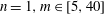
The POD modes in the azimuthal direction are harmonic and simply described with a set of sine waves and are therefore inherently self-similar. As mentioned in § 3, the modes in the temporal and streamwise directions are also self-similar, as they too are harmonic. The modes in the radial direction, however, are driven by the dataset and are not known a priori to solving the eigenvalue problem. Here, we will address the self-similarity in the azimuthal and radial directions and the existence of a universal length scale.

The size of the eddy is estimated by its azimuthal and radial length scales. The wall-normal length scale is estimated as the radius of the eddy in the wall-normal direction, here measured as the distance from the wall to the peak location of the first POD mode for the investigated azimuthal mode number, ${\it\Phi}^{(1)}(m;r)$ . The azimuthal wavelength is estimated as ${\it\lambda}_{{\it\theta}}=2{\rm\pi}R_{p}/m$ , where $R_{p}=(R-y_{p})$ and $y_{p}$ is the wall-normal location of the mode maximum. Figure 5 shows the wall-normal length scale, $y_{p}/R$ , and the azimuthal wavenumber, $k_{{\it\theta}}R=2{\rm\pi}R/{\it\lambda}_{{\it\theta}}$ , for the eddies resolved within the first POD mode and azimuthal mode numbers $m\in [1,64]$ , where the square brackets indicate the range of mode numbers. The azimuthal mode number is indicated on the upper abscissa, where the axis was mapped using $k_{{\it\theta}}R=m(R_{p}/R)$ and $R_{p}/R$ was taken from the modes obtained from the $Re_{{\it\tau}}=2460$ data.

Figure 5. The modal peak locations for the first POD mode $(n=1)$ and azimuthal mode numbers $m\in [1,64]$ : ▴,  $Re_{{\it\tau}}=1330$ ; ▪,  $Re_{{\it\tau}}=2460$ ; $\cdots \cdots$ , $y_{p}/R=2{\rm\pi}C(k_{{\it\theta}}R)^{-1}$ , with $C=0.2$ . Modes with a peak location $y_{p}^{+}<75$ are identified with open symbols. The lower abscissa indicates the azimuthal wavenumber, while the upper abscissa shows the corresponding azimuthal mode number, for $Re_{{\it\tau}}=2460$ .

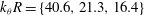
The aspect ratio of the eddy can be defined as $y_{p}/{\it\lambda}_{{\it\theta}}$ and is constant for all self-similar eddies. Hence, $y_{p}/R=2{\rm\pi}C(k_{{\it\theta}}R)^{-1}$ , where the constant $C$ is estimated to be 0.2 to fit the data in figure 5, see the dotted line. The eddies exhibit a self-similar behaviour for almost a decade, with wavenumbers $k_{{\it\theta}}R\in [4.29,22.3]$ (or $m\in [3,21]$ ) with corresponding wall-normal distance 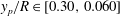$y_{p}/R\in [0.30,0.060]$ , for $Re_{{\it\tau}}=1330$ . At $Re_{{\it\tau}}=2460$ , the structures stay self-similar for a wider span, with 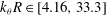$k_{{\it\theta}}R\in [4.16,33.3]$ ( $m\in [3,32]$ ), with 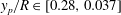$y_{p}/R\in [0.28,0.037]$ (see table 1). In this region, the wall-normal distance $y_{p}$ is the appropriate length scale for both directions.

The deviation of the larger eddies $(m\in \{1,2\})$ is expected to be caused by the pipe geometry, as the larger eddies are more influenced by the pipe curvature (Chung et al. Reference Chung, Marusic, Monty, Vallikivi and Smits2015). The smaller eddies, estimated by $y_{p}^{+}<75$ , are influenced by the viscosity and are indicated with open symbols in figure 5. It should be noted that the aspect ratio stays constant for eddies reaching far into the wake region, with the centre of the largest self-similar eddy, $(n,m)=(1,3)$ , located at $y/R=0.28$ .

Figure 5 shows the self-similarity of the mode peak locations, while the self-similarity of the radial POD modes themselves is shown in figure 6. The magnitude of the scaled POD modes, $\widehat{{\it\Phi}}^{(n)}(m;r)$ , has been rescaled using its maximum value, instead of its $L^{2}$ -norm as in figure 2. The wall-normal direction should be scaled with the eddy radius, characterized by the distance from the wall to its peak location. As this distance is sensitive to any offset in the wall location, the eddy size was instead estimated by the distance from the peak location to the outer edge of the eddy. The outer edge was identified as the location where the magnitude of the POD mode reaches 5 % of its peak value, $y_{5}$ . All modes in figure 6 are scaled using the length scale estimated from the first POD mode for any given azimuthal mode, shown in figure 6(a). The scaled modes are insensitive to the chosen threshold within the range 2.5 % to 10 % of the peak value.

Figure 6. The scaled modal profiles of the streamwise component for the radial POD modes: (a) $n=1,m\in [5,40]$ ; (b) $n=1,m\in [5,35]$ ; (c) $n=2,m\in [5,40]$ ; (d) $n=2,m\in [5,20]$ ; (e) $n=3,m\in [5,40]$ ; (f) $n=3,m\in [5,15]$ . Here, $Re_{{\it\tau}}=2460$ .

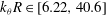
The scaled first, second and third POD modes, for $k_{{\it\theta}}R\in [6.22,40.6]$ , are shown in figure 6(a), (c) and (e) respectively. The first three POD modes show a clear collapse for the near-wall eddies, for all azimuthal wavenumbers, while the higher order POD modes $(n>1)$ show deviations for the eddies farther from the wall. The eddies farther from the wall do show a collapse when excluding the higher wavenumber modes, figure 6(d,f). Although these eddies are physically detached from the wall in the sense that there are eddies, of opposite sign, present closer to the wall, they are attached in the sense of Townsend; they can be scaled using a single length scale estimating their size as their distance from the wall. Moreover, the modes exhibiting self-similarity are the lower-order azimuthal modes, while the higher-order azimuthal modes show relatively weaker outer structures. The higher limit of the azimuthal wavenumber is estimated by eye to be $k_{{\it\theta}}R=\{40.6,21.3,16.4\}$ for the first, second and third POD modes respectively. Hellström et al. (Reference Hellström, Ganapathisubramani and Smits2015) related the combination of the first three POD modes to the hairpin packets and the transition between consecutive structures. Figure 6 suggests that there is a lower limit to the size of the packets for which they can detach; hence, the physically detached eddies are getting weaker relative to their near-wall counterparts.

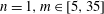
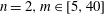
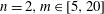
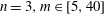
The two-dimensional reconstruction of the self-similar modes can be seen in figure 7. Figure 7(a,c,e) shows the largest of the self-similar eddies, $m=5$ , while figure 7(b,d,f) shows the smallest of the self-similar eddies, for each respective POD mode. The white marks indicate $y_{p}$ and $y_{5}$ , which are used as the fixed points for the scaling. The first POD modes can be seen in figure 7(a,b), where a strong similarity is maintained despite the large difference in eddy size. The larger of the eddies is 6.71 times and 3.51 times larger in the azimuthal and wall-normal directions respectively.

Figure 7. Scaled modes: (a) $(n,m)=(1,5)$ , (b) $(n,m)=(1,40)$ , (c) $(n,m)=(2,5)$ , (d)  $(n,m)=(2,20)$ , (e) $(n,m)=(3,5)$ , (f) $(n,m)=(3,15)$ . White represents positive and black negative values; the white marks indicate the points used for scaling.

5 Discussion and conclusions

The energetic POD modes in turbulent pipe flows have previously been shown to be associated with the large-scale motions, where the first three radial POD modes represent the same coherent structure at different stages of its evolution, initiation, growth and wall detachment. During this evolution, the POD modes maintain its azimuthal wavelength, which is known a priori to the POD evaluation. Here, we provide evidence that these POD modes exhibit a self-similar behaviour, where there is a single length scale representing the complete structure. This geometric self-similarity of the energy-containing motions directly supports the recent findings of Hwang (Reference Hwang2015) and is inherent to models based on Townsend’s attached eddy hypothesis.

The eddies are found to exhibit a self-similar behaviour, with the azimuthal wavenumbers of the largest to the smallest eddies spanning a decade. The centre of the largest self-similar eddy reaches far into the wake region and is located at $y/R=0.28$ . The modes resolving the energetic eddies in the homogeneous directions are the harmonic ones, and thus are inherently self-similar. In the wavenumber range $k_{{\it\theta}}R\in [4.16,33.3]$ , where the only non-homogeneous directions also are self-similar, all eddies can be fully described with a single radial profile. The length scale representing the eddy is estimated by its wall-normal radius, which is the universal length scale completely describing the cross-sectional shape or the structure through all stages of its evolution. However, with the current dataset, we are unable to verify whether the wall-normal length scale is the appropriate streamwise length scale.