


1. Introduction
The intrinsic multiscale features present in many natural and industrial processes, including cavitation and bubble growth (Ghahramani, Arabnejad & Bensow Reference Ghahramani, Arabnejad and Bensow2019), advanced functional materials (Chen et al. Reference Chen, Kuang, Zhu, Burgert, Keplinger, Gong, Li, Berglund, Eichhorn and Hu2020) and lithium-ion batteries (Abada et al. Reference Abada, Marlair, Lecocq, Petit, Sauvant-Moynot and Huet2016), originate from nanometre-to-millimetre phenomena across a wide range of temporal and spatial scales. In general, even for the same physical system, the dominant factors in the microscale and macroscale dynamic processes may be different. Taking the bubble growth dynamics as an example, at the macroscale, we can apply the continuum hypothesis, assume spherical bubbles and constant surface tension, ignore the compressibility of the surrounding fluid and all stochastic effects to derive the Rayleigh–Plesset model (Plesset & Prosperetti Reference Plesset and Prosperetti1977). However, at the microscale, the bubble surface can exhibit thermal waves (Aarts, Schmidt & Lekkerkerker Reference Aarts, Schmidt and Lekkerkerker2004), the surrounding fluid is compressible (Zhao, Xia & Cao Reference Zhao, Xia and Cao2020) and thermally induced fluctuations (Baidakov & Protsenko Reference Baidakov and Protsenko2020) could play an important role in the dynamic processes. Therefore, to correctly consider significantly different dominant physics across scales, we have to employ multiple physical models expressed in different mathematical forms each for a specific band of spatio-temporal scales (Goel et al. Reference Goel2020). For instance, molecular dynamics (MD) models are governed by Newton's equations of motion and are limited to submicron phenomena, while macroscale models in the form of partial differential equations derived from the continuum hypothesis work well in the continuum limit but often breakdown at the microscale. Consequently, correct physics at multiple and disparate scales should be described by appropriate physical models expressed in mathematical forms that can be computationally solvable. However, simulating multiscale problems with coupled nanoscale processes and macroscale material response over several decades or more of spatio-temporal scales is beyond the capability of any single simulation solver (Yip & Short Reference Yip and Short2013). Multiscale modelling that couples heterogeneous physical models at different scales is a key to creating more accurate predictive tools for analysis of multiscale phenomena.
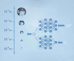
To concurrently couple different physics across scales, the concept of handshaking has been widely used in traditional multiscale simulations to communicate essential information between scales, where two adjoint domains with different scales and resolutions are linked together through an overlapped region (or handshake region) (Gooneie, Schuschnigg & Holzer Reference Gooneie, Schuschnigg and Holzer2017). Figure 1 presents a handshaking example of the cavitation and bubble growth dynamics. In the continuum limit ( $>10^{-6}\,\textrm {m}$), the Rayleigh–Plesset (R–P) model derived from the Navier–Stokes equations under the assumption of spherical symmetry can be used to describe how a bubble grows in response to pressure changes. In the atomistic regime (
 $<10^{-6}\,\textrm {m}$), where the stochastic effects and interfacial fluctuations can play an important role in bubble dynamics, a two-phase dissipative particle dynamics (DPD) model can be used to simulate the bubble growth dynamics. To investigate the full-scale phenomena of cavitation and bubble growth, a handshaking algorithm should be adopted to couple the continuum regime and the stochastic regime at the demarcation boundary around
  $10^{-6}\,\textrm {m}$. Many handshake algorithms have been developed and successfully applied to diverse multiscale problems, i.e. coupling of atomistic and coarse-grained scales for crack growth in silicon (Budarapu et al. Reference Budarapu, Javvaji, Reinoso, Paggi and Rabczuk2018), coupling of MD and DPD for functionalized surfaces (Wang et al. Reference Wang, Li, Xu, Yang and Karniadakis2019) and coupling of the classical density functional theory and the continuum-based Poisson–Nernst–Planck equations for charged fluids (Cheung et al. Reference Cheung, Frischknecht, Perego and Bochev2017). The triple-decker algorithm for fluid flows proposed by Fedosov & Karniadakis (Reference Fedosov and Karniadakis2009) couples the MD with DPD and the Navier–Stokes equations in a tri-layer structure. However, multiscale production simulations are still rare in engineering applications due to the lack of appropriate frameworks that unify multiscale models and streamline the multiscale modelling process despite recent progress (Tang et al. Reference Tang, Kudo, Bian, Li and Karniadakis2015).

Figure 1. Multiscale bubble growth problem, from the scale of nucleation to a centimetre. To model this process, different methods are needed at different scales, e.g. the Rayleigh–Plesset model on the macroscale and dissipative particle dynamics on the microscale. The ‘handshaking’ problem involves coupling between the two physical models involving different mathematical descriptions at the demarcation boundary around 1  $\mathrm {\mu }\textrm {m}$.
Machine learning (ML)-based approaches, especially neural network models, have achieved remarkable successes recently in diverse scientific applications (Peng et al. Reference Peng2021). Learning the governing equations or operators from data makes it possible to uncover an appropriate multiscale approach valid across scales for complex problems. In the present work, we develop a supervised ML approach named DeepONet to learn effective operators for multiscale physics from mixed mean-field and stochastic simulation data. DeepONet drastically simplifies the multiscale modelling procedure by eliminating the handshaking processes in traditional multiscale modelling and unifying multiple physical models across scales. This, in turn, will allow modellers to explore the hidden physics in multiscale data and establish pathways between data-driven research and physics-based research for multiscale and multiphysics problems.
In previous work in Lin et al. (Reference Lin, Li, Lu, Cai, Maxey and Karniadakis2021), we demonstrated that using different DeepONets we can train them separately to predict the bubble growth dynamics either in the continuum or atomistic regimes with good accuracy. However, the challenging question is if a single DeepONet can learn the dynamics simultaneously from both regimes and therefore predict seamlessly the growth of nanobubbles or millibubbles. This is the problem we are tackling in this work, starting from the data generation, the required training in a properly scaled spatio-temporal domain and the validation of the method based on testing and predictions for unseen pressure data and unseen initial bubble radius.
2. Data generation
2.1. DPD (stochastic regime)
The DPD model was introduced by Hoogerbrugge & Koelman (Reference Hoogerbrugge and Koelman1992). It is considered as one of the coarse-grained approaches of MD simulation. As with MD systems, a DPD model consists of many interacting particles governed by Newton's equation of motion (Groot & Warren Reference Groot and Warren1997),
 \begin{equation} m_i\frac{\textrm{d}^{2}\boldsymbol{r}_i}{\textrm{d}t^{2}} = m_i\frac{\textrm{d}\boldsymbol{v}_i}{\textrm{d}t} = \boldsymbol{F}_i = \sum_{j\ne i}\left(\boldsymbol{F}^{C}_{ij} + \boldsymbol{F}^{D}_{ij} + \boldsymbol{F}^{R}_{ij}\right), \end{equation}
where  $m_i$ is the mass of a particle
  $i$,
$i$,  $\boldsymbol {r}_i$ and
  $\boldsymbol {v}_i$ are the position and velocity vectors of particle
  $i$ and
  $\boldsymbol {F}_i$ is the total force acting on the particle
  $i$ due to the presence of neighbouring particles. The summation for computing
  $\boldsymbol {F}_i$ is carried out over all neighbouring particles within a cutoff range. The pairwise force is comprised of a conservative force
  $\boldsymbol {F}^{C}_{ij}$, a dissipative force
  $\boldsymbol {F}^{D}_{ij}$ and a random force
  $\boldsymbol {F}^{R}_{ij}$, given in the following forms:
 \begin{equation} \left. \begin{aligned} & \boldsymbol{F}^{C}_{ij} = a_{ij}\omega_C(r_{ij})\boldsymbol{e}_{ij}, \\ & \boldsymbol{F}^{D}_{ij} ={-}\gamma_{ij}\omega_D(r_{ij})(\boldsymbol{v}_{ij}\boldsymbol{e}_{ij})\boldsymbol{e}_{ij}, \\ & \boldsymbol{F}^{R}_{ij}\boldsymbol{\cdot} \textrm{d}t = \sigma_{ij}\omega_R(r_{ij})\,\textrm{d}\tilde{W}_{ij}\boldsymbol{e}_{ij}, \end{aligned} \right\} \end{equation}
where  $r_{ij}=|\boldsymbol {r}_{ij}| = |\boldsymbol {r}_i-\boldsymbol {r}_j|$ is the distance between particles
  $i$ and
  $j$,
$j$,  $\boldsymbol {e}_{ij}=\boldsymbol {r}_{ij}/r_{ij}$ is the unit vector,
  $\boldsymbol {v}_{ij} = \boldsymbol {v}_i-\boldsymbol {v}_j$ is the velocity difference and
  $\textrm {d}\tilde {W}_{ij}$ is an independent increment of the Wiener process (Español & Warren Reference Español and Warren1995). The coefficients
  $a_{ij}$,
  $\gamma _{ij}$ and
  $\sigma _{ij}$ determine the strength of the three forces, respectively. To satisfy the fluctuation–dissipation theorem (Español & Warren Reference Español and Warren1995), the dissipative force and the random force are constrained by
  $\sigma _{ij}^{2} = 2\gamma _{ij}k_BT$ and
  $\omega _D(r_{ij})=\omega ^{2}_R(r_{ij})$.
With the purely repulsive conservative forces, DPD is most suitable for simulating a gas, which fills the space spontaneously. To simulate the liquid phase, we use the many-body DPD (MDPD), which is an extension of DPD by modifying the conservative force to include both an attractive force and a repulsive force (Warren Reference Warren2003; Arienti et al. Reference Arienti, Pan, Li and Karniadakis2011),
 \begin{equation} \boldsymbol{F}_{ij}^{C} = A_{ij}w_c(r_{ij}) + B_{ij}(\rho_i + \rho_j) w_d(r_{ij}). \end{equation}
Since a DPD model with a single interaction range cannot maintain a stable interface (Pagonabarraga & Frenkel Reference Pagonabarraga and Frenkel2001), the repulsive contribution is set to act within a shorter range  $r_d < r_c$ than the soft pair attractive potential. The many-body repulsion is chosen in the form of a self-energy per particle, which is quadratic in the local density,
  $B_{ij}(\rho _i+\rho _j)w_d(r_{ij})$, where
  $B_{ij}>0$. The density of each particle is defined as
 \begin{equation} \rho_i = \sum_{j \neq i}w_{\rho}(r_{ij}), \end{equation}
and its weight function  $w_{\rho }$ is defined as
 \begin{equation} w_{\rho}=\frac{15}{2 {\rm \pi}r_d^{3}}\left(1-\frac{r}{r_d}\right)^{2}, \end{equation}
where  $w_\rho$ vanishes for
  $r > r_d$.
Figure 2(a) illustrates the DPD–MDPD coupled simulation system, where the traditional DPD particles (yellow) are used for the gas phase and MDPD particles (blue) for the liquid phase. The model has been validated by comparing it with the R–P equation for the larger size bubbles and with MD for the smaller size bubbles (Pan et al. Reference Pan, Zhao, Lin and Shao2018). To reduce the computational cost, a thin box with periodic boundaries in the  $x$ and
  $z$ directions is used. To change the system pressure, the top and bottom walls are set to have one degree of freedom moving just in the
  $y$ direction. The external force (green arrows) on the walls evolves following a preset function. We continuously monitor the volume of the gas phase and use it to compute the effective bubble radius. Specifically, we adopt a Voronoi tessellation (Rycroft Reference Rycroft2009) to estimate the instantaneous volume occupied by the gas particles. The particle density ratio of liquid to gas is
  $5.0$. More details of the DPD simulations can be found in our preliminary work (Lin et al. Reference Lin, Li, Lu, Cai, Maxey and Karniadakis2021).

Figure 2. (a) The DPD system at the microscale. The blue particles represent the liquid phase while the yellow particles represent the gas phase. Time-varying external forces are exerted on both the top and bottom walls to control the system pressure. The bubble radius,  $R(t)$, is computed by measuring the volume occupied by the gas particles. (b) The R–P model at macroscale. A circular bubble is at rest in liquid. The change of pressure,
  $\Delta P(t)$, at the boundary at
  $R_E$ induces the change to the bubble size. (c) Value of
  $R(t)$ of an initial bubble of radius 1.258
  $\mathrm {\mu }\textrm {m}$ responding to
  $\Delta P(t)$; the inset shows
  $\Delta P(t)$. The comparison of the R–P solution and the mean DPD simulation results shows a discrepancy of
  $1.8\,\%$. (d) When the bubble size is 92.4 nm, the discrepancy increases to over
  $15\,\%$. For a fair comparison,
  $\Delta P(t)$ values are the same. Such systematic comparisons suggest that 1
  $\mathrm {\mu }\textrm {m}$ is a reasonable demarcation boundary between the R–P and the DPD models.
2.2. The R–P model (continuum regime)
The standard R–P equation (Plesset & Prosperetti Reference Plesset and Prosperetti1977) is derived from the continuum-level Navier–Stokes equations. It describes the change in radius  $R(t)$ of a single, spherical gas-vapour bubble in liquid as the far-field pressure,
  $p_{\infty }(t)$, varies with time
  $t$. In order to be consistent with the mean-field dynamics of the DPD system, we develop a new two-dimensional (2-D) version of the R–P model for a gas bubble in a finite body of liquid with a finite gas–liquid density ratio. The schematic of this model is depicted in figure 2(b), showing a circular gas bubble with radius
  $R$ inside an external circular boundary with radius
  $R_{E}$. The external boundary is needed as there is no finite limit for the fluctuating pressure as
  $r \to \infty$. Here,
  $R_{E}$ is determined by matching the volume of the liquid between the R–P system and the DPD system.
We consider first the motion in the surrounding liquid, which we assume to be incompressible, with constant density  $\rho _L$ and viscosity
  $\mu _L$. As the bubble expands, there is a radial potential flow
  $u(r, t)$ that matches the kinematic conditions at
  $r = R$ and
  $r = R_E$ such that
 \begin{gather} u(R, t) = \frac{\mathrm{d} R}{\mathrm{d} t} \end{gather}
 \begin{gather}u(R_E,t) = \frac{\mathrm{d} R_E}{\mathrm{d} t} = \frac{R}{R_E} \frac{\mathrm{d} R}{\mathrm{d} t}. \end{gather}
The latter determines  $R_E (t)$ and ensures that
  ${\rm \pi} (R_E^{2} - R^{2}) = V_L$ is constant, where
  $V_L$ is the liquid volume per unit length in
  $z$. The pressure in the liquid is found from the Navier–Stokes equation with
  $u=R/r \cdot \mathrm {d}R/\mathrm {d}t$, and up to some arbitrary function
  $g(t)$
 \begin{equation} -p_{L} (r,t) = \rho_{L} \left \{ \frac{\mathrm{d}}{\mathrm{d}t} \left( R\frac{\mathrm{d}R}{\mathrm{d}t} \right) \log r + \frac{u^{2}}{2} \right \} + g(t). \end{equation}
The liquid pressure at  $r=R_E$ is specified as
  $p_{L} (R_E,t) = p_{E} (t)$. At
  $r=R$, the difference in the normal stresses balances the surface tension,
 \begin{equation} \left.\left\{{-}p_{L} + 2\mu_{L} \frac{\partial u}{\partial r} \right \} \right|_{R+} + \frac{\gamma}{R} = \tau^{B}_{rr}(t), \end{equation}
where  $\gamma$ is the coefficient of surface tension at the gas–liquid interface and
  $\tau ^{B}_{rr}(t)$ is the normal stress in the gas phase at the bubble surface.
If we neglect the inertia and the viscous stresses of the gas phase, the only contribution to the normal stress is the gas pressure,  $\tau ^{B}_{rr}(t) = -p_B(t)$. The resulting 2-D R–P model for a circular gas bubble is
 $$\begin{gather} p_B(t) - p_{L} (R_E,t) = \rho_{L}\log_{e}\left(\frac{R_E}{R}\right)\frac{\textrm{d}}{\textrm{d}t}\left(R\frac{\textrm{d}R}{\textrm{d}t}\right) - \frac{1}{2}\rho_L\left(1-\frac{R^{2}}{R_{E}^{2}}\right)\left(\frac{\textrm{d}R}{\textrm{d}t}\right)^{2} \nonumber\\ + 2 \mu_L \frac{1}{R}\frac{\mathrm{d}R}{\mathrm{d}t} + \frac{\gamma}{R}. \end{gather}$$
Within the bubble, the thermodynamic pressure of the gas is assumed to be given by a polytropic gas law,
 \begin{equation} {p_{B}(t) = p_{G0} \left(\frac{T_B}{T_\infty}\right) \left(\frac{R_0}{R}\right)^{k}}, \end{equation}
where  $k$ is approximately constant and related to the system state. A number of quasi-static DPD simulations were conducted at different liquid pressures to calibrate
  $k$ and a value of
  $k = 3.68$ was obtained as a best fit to the simulation data over the working range. The DPD simulations employ a thermostat to maintain stability of the simulations and so the system may be considered to be approximately isothermal. Although the temperature of an oscillating bubble may be changed by viscous heating or pressure work, in the present study, we consider that the fluid system is connected to a thermostat bath to maintain a constant system temperature, and thus we neglect the effect of temperature difference between the gas and the liquid, setting
  $T_{B} = T_{\infty }$. For both the DPD simulations and the R–P model, the initial conditions are that the gas bubble is in a thermal equilibrium state at
  $t = 0$ with an initial radius of
  $R_0$, a gas pressure
  $p_{G0}$ and a liquid pressure
  $p_{L}(0)=p_{E}(0)$. The initial gas and liquid pressures satisfy the 2-D Young–Laplace equation
 \begin{equation} {p_{G0} = p_{L}(0)+\frac{\gamma}{R_{0}}}. \end{equation}
In the initial equilibrium state, any inertial effect of the gas phase can be neglected because  $\textrm {d}R/\textrm {d}t|_{t=0}=0$.
For the present DPD simulations, the gas–liquid density ratio is not negligible,  $\rho _G / \rho _L \sim 0.2$ and so the motion in the gas phase needs to be considered. In principle, this is a compressible flow, but the time scale for pressure waves to traverse the bubble
  $R/c_G$, where
  $c_G$ is the sound speed in the gas phase, is very short compared with the other processes. In other words, the Mach number
  $\epsilon = u(R,t)/c_G \ll 1$. This is in keeping with other compressible R–P models (Prosperetti & Lezzi Reference Prosperetti and Lezzi1986; Fuster, Dopazo & Hauke Reference Fuster, Dopazo and Hauke2011; Wang Reference Wang2014), where the focus is on pressure waves in the liquid at large distances from the bubble and where conditions in the near field are still essentially incompressible. So as the gas bubble expands, the first approximation is that the local rate of expansion is the same at all points within the bubble. There is again a radial potential flow,
  $\boldsymbol {u} = \boldsymbol {\nabla } \phi$ with
 \begin{gather} \nabla^{2} \phi = \frac{2}{R} \frac{\mathrm{d} R}{\mathrm{d}t}, \end{gather}
 \begin{gather}u(r,t) = \frac{r}{R} \frac{\mathrm{d} R}{\mathrm{d}t}. \end{gather}
 Correspondingly, the density of the gas  $\rho _G (t)$ is uniform within the bubble and relative to the initial conditions,
 \begin{equation} \rho_G(t) = \rho_{G0} (R_0 / R(t) )^{2}. \end{equation}
 The pressure is primarily the thermodynamic pressure as given by  $p_{B}(t)$ with an additional small correction due to the fluid motion in the gas phase,
  $p_{1} (r, t)$ and
  $p_G(r,t) = p_B(t) + p_{1} (r, t)$. These pressure variations are not sufficient to modify the gas density appreciably if
  $\epsilon \ll 1$, and corrections to the density would be higher order in
  $\epsilon$. The pressure variation can be found from the Navier–Stokes equation, along with a Stokes model for the bulk viscosity, as
 \begin{equation} p_1(r,t) = f(t) - \frac{\rho_G(t)}{2R} r^{2} \frac{\mathrm{d}^{2}R}{\mathrm{d}t^{2}}. \end{equation}
Here, there is an arbitrary function  $f(t)$ from the integration. We could choose to set
  $p_1(0,t)=0$ and use the centre of the bubble as the reference point. Instead, we set the average value of
  $p_1$ within the bubble to be zero, leaving
  $p_B$ as the average pressure in the bubble. This is consistent with the way the gas pressure in the bubble is evaluated in the DPD simulations. The result is,
 \begin{equation} 0=\int_{0}^{R}2{\rm \pi} rp_2(r,t)\mathrm{d}r ={-}\rho_1(t)\left ( \frac{1}{2R} \frac{\mathrm{d}^{2}R}{\mathrm{d}t^{2} } \right ) \frac{{\rm \pi} R^{4}}{2} + {\rm \pi}R^{2} f(t). \end{equation}
These results may be combined to give a corrected estimate for the normal stress in the gas phase at the bubble surface,
 \begin{equation} \tau^{B}_{rr}(t) ={-}p_B(t) +\frac{1}{4} \rho_G (t) R \frac{\mathrm{d}^{2}R}{\mathrm{d}t^{2} } + 2 \mu_G \frac{1}{R}\frac{\textrm{d}R}{\textrm{d}t}. \end{equation}
Finally, the modified version of the 2-D R–P equation that includes the gas flow in the bubble is
 \begin{align} &p_B(t) - \frac{1}{4}\rho_{G}(t) R \frac{\mathrm{d}^{2}R}{\mathrm{d}t^{2}} - p_{L}(R_E,t) \nonumber\\ &\quad = \rho_L \log_e \left ( \frac{R_E}{R} \right ) \frac{\mathrm{d}}{\mathrm{d}t}\left ( R \frac{\mathrm{d}R}{\mathrm{d}t} \right ) - \frac{1}{2}\rho_L \left ( 1-\frac{R^{2}}{R_E^{2}} \right ) \left ( \frac{\mathrm{d}R}{\mathrm{d}t} \right )^{2} \nonumber\\ &\qquad + \left ( 2\mu_L + \frac{2}{3}\mu_G \right ) \frac{1}{R} \frac{\mathrm{d}R}{\mathrm{d}t} + \frac{\gamma}{R}. \end{align}
This equation is used in the present study. It should be noted that the DPD simulations give the average force on the upper and lower walls, which are no-slip boundaries (Lin et al. Reference Lin, Li, Lu, Cai, Maxey and Karniadakis2021). As these are flat surfaces and the liquid is essentially incompressible, there is no normal viscous stress and the average force will correspond to the liquid pressure. For this reason, we do not consider the viscous normal stress at  $r = R_E$ and simply relate
  $R(t)$ to
  $p_{E} (t)$.
3. DeepONet
Our work is inspired by the work of Lu et al. (Reference Lu, Jin, Pang, Zhang and Karniadakis2021a), who proposed a deep operator network (DeepONet) to approximate nonlinear continuous operators. The DeepONet architecture is based on rigorous mathematical theory, namely the universal operator approximation theorem (Chen & Chen Reference Chen and Chen1995), which has been extended to deep neural networks (DNNs).
In order to test whether DeepONet can represent a unified surrogate model for multiscale problems, first, we need to define a reasonable multiscale spatio-temporal domain for training. Figure 3(a) shows an example domain, which we designed for the bubble dynamics problem. In this spatio-temporal domain, the length scale equals to  $R_0$, and the time scale equals to the whole time interval,
  $T$. The domain has a shape of trapezoid, meaning that
  $T$ for different
  $R_0$ is different. It is not only physically meaningful but also practical to make the time scale linked to the length scale, and it greatly expedites the training process.

Figure 3. (a) The spatio-temporal domain for operator regression. The length scale equals to the initial bubble radius,  $R_0$. The upper and lower boundary values for
  $R_0$ are 100 nm and 10
  $\mathrm {\mu }\textrm {m}$, respectively. The time scale equals to the whole time interval,
  $T$. The boundary of
  $T$ is related to
  $R_0$ by defining a dimensionless characteristic time,
  $\tau _c$, so that
  $T_{\tau _c} = 5$ in all the different regimes. The training data are composed of two parts: when
  $R_0$ is between 1 and 10
  $\mathrm {\mu }\textrm {m}$ data are generated by the R–P model, while when
  $R_0$ is between 100 nm and 1.25
  $\mathrm {\mu }\textrm {m}$ data are generated by the DPD model. The demarcation region is between 1 and 1.25
  $\mathrm {\mu }\textrm {m}$ and contains data from both physical models. (b) The architecture of DeepONet. The branch net takes
  $\Delta P$ as input while the trunk net takes
  $R_0$ and time
  $t$ as input. The output of the network is the relative bubble size change.
Next, we introduce the characteristic time  $\tau _c$, defined as
  $\tau _c=(\rho R_{0}^{2} / \Delta P_c)^{{1}/{2}}$, where
  $\Delta P_c$ is the characteristic pressure change. With the help of
  $\tau _c$, we can transform the trapezoid domain to a regular domain. Take figure 3(a) for example, a different physical time
  $T$ can be described by the same corresponding dimensionless time,
  $T_{\tau _c} = 5$. The transformed regular domain will be used to train DeepONet later.
In this example problem, we set limits for  $R_0$, i.e. the upper and lower boundaries 10
  $\mathrm {\mu }\textrm {m}$ and 100 nm, and set the corresponding
  $T = 50\,\mu \textrm {s}$ and 500 ns, in other words,
  $T_{\tau _c} = 5$ for all
  $R_0$. According to the simulations (see figure 2c,d), we set the demarcation boundary between two physical models at the scale of 1
  $\mathrm {\mu }\textrm {m}$. Specifically, data with
  $R_0$ between 100 nm and 1.25
  $\mathrm {\mu }\textrm {m}$ are generated by the DPD simulations, while data with
  $R_0$ between 1 and 10
  $\mathrm {\mu }\textrm {m}$ are generated by the R–P model. The data in the handshaking region (between 1 and 1.25
  $\mathrm {\mu }\textrm {m}$) are a mix of data from both physical models. The data from two sources can be simply concatenated or even arbitrarily blended as the order of mixing has no effect on DeepONet.
The liquid pressure is set to be randomly time varying and drawn from a Gaussian random process ( $\mathcal {GP}$), with an exponential function mask ensuring a smooth transition from the initial equilibrium state (
 $P_{L}(0)=2.93\times 10^{6}\,\textrm {Pa}$). We define the liquid pressure variation
  $\Delta P(t)$, as
 \begin{equation} \left. \begin{aligned} & g(t) \sim \mathcal{GP}(\mu, \sigma k_{lT}(t_1, t_2)), \\ & s(t) = \begin{cases} \left( \dfrac{t}{qT} \right)^{10} & 0 \leq t < qT, \\ 1 & qT \leq t \leq T, \\ \end{cases} \\ & \Delta P(t) = g(t)s(t), \\ \end{aligned} \right\} \end{equation}
where the mean of the variation  $\mu =0 \,\textrm {Pa}$ and the standard deviation
  $\sigma =9.76\times 10^{5}\,\textrm {Pa}$, the parameter
  $\sigma$ is also used to set the value of
  $\Delta P_c$ in
  $\tau _c$. The Gaussian covariance kernel
  $k_{lT}(t_1, t_2) = \exp (-\| t_1 - t_2 \|^{2} / 2l^{2}T^{2})$ has a correlation time scale based on the time-scale parameter
  $lT > 0$. The dimensionless parameter
  $l$ determines the smoothness of the sampled function and we choose
  $l=0.2$ in this study. A systematic study on the effect of the correlation length can be found in (Lin et al. Reference Lin, Li, Lu, Cai, Maxey and Karniadakis2021). The parameter
  $q$ controls the pressure transition period and we set
  $q=0.1$.
The architecture of the DeepONet is shown in figure 3(b); it consists of a DNN for encoding the discrete input function space (branch net) and another DNN for encoding the coordinates of the output functions (trunk net). For the multiscale bubble dynamics application, the input function is  $\Delta P$, while the output function is the relative bubble radius change
  $(R(t)-R_0)/R_0$. There are different ways to represent a function but here the input to the branch is represented by discrete function values at a sufficient but finite number of locations, which we call ‘sensors’. The architecture we used in this study is shown in figure 3(b). The trunk network takes initial bubble radius
  $R_0$ and time
  $t$ as the input and outputs
  $[a_1,a_2,\ldots,a_p]^\textrm {T}$. The branch network takes
  $[\Delta p(t_1),\Delta p(t_2),\ldots,\Delta p(t_m)]^\textrm {T}$ as the input and outputs a vector
  $[b_1,b_2,\ldots,b_p]^\textrm {T}$. This architecture corresponds to the unstacked DeepONet (Lu et al. Reference Lu, Jin, Pang, Zhang and Karniadakis2021a). Then, the two vectors are merged together to predict the relative bubble radius change:
  $(R(t)-R_0)/R_0 = G(\Delta P)(R_0)(t) = \varSigma ^{p}_{k=1}b_{k}a_{k}$.
For each input function,  $\Delta P$, DeepONet requires evaluations at the same set of discrete times. However, DeepONet does not have any constraint on the number or location of the evaluation of the output function,
  $(R(t)-R_0)/R_0$. In this study, for the efficient training of the networks, we choose a fixed number of evaluations for each output function but at randomly selected times within the whole interval.
To generate the training data,  $10$ DPD systems are constructed with different
  $R_0$ ranging from 100 nm to 1.25
  $\mathrm {\mu }\textrm {m}$, denoted by blue dots in figure 3(a). For each
  $R_0$,
  $50$ different
  $\Delta P(t)$ are considered. So a total of
  $500$ pairs of input
  $\Delta P(t)$ and output
  $R(t)$ are generated by the DPD model. Technically, in order to average the inherent thermal fluctuations of DPD simulation, each
  $R(t)$ is the ensemble average of
  $12$ separate simulations. Similar to DPD, the R–P model is used to generate
  $500$ pairs of input
  $\Delta P(t)$ and the resulting
  $R(t)$ with
  $10$ fixed
  $R_0$. The
  $10$ discrete values of
  $R_0$ are shown in figure 3(a) with orange dots.
Following the best practice of our preliminary study (Lin et al. Reference Lin, Li, Lu, Cai, Maxey and Karniadakis2021), the training dataset takes  $50$ evenly spaced points on the input function,
  $P(t)$, and
  $50$ randomly spaced points on the output function,
  $(R(t)-R_0)/R_0$. It is worth noting that, because
  $T$ depends on
  $R_0$ in this spatio-temporal domain, fetching
  $50$ sample points from the output function means that the time step or sampling density is automatically dependent on
  $R_0$. However, from the perspective of
  $\tau _c$ units, the sampling density is always the same.
The loss function we employ is the mean squared error between the true value and the network prediction. We apply the Adam optimizer with a small learning rate  $5\times 10^{-4}$ to train the DeepONet for
  $2\times 10^{5}$ iterations. The rectified linear unit is used for the activation function. The width and depth of both the branch and trunk net are
  $200$ and
  $3$. We use a feedforward neural network as the architecture of the two sub-networks, which are implemented in the Python library DeepXDE (Lu et al. Reference Lu, Meng, Mao and Karniadakis2021b).
4. Results
Upon training, we test DeepONet on unseen  $R_0$ and unseen
  $\Delta P(t)$. Figure 4 shows some examples. Here, the DeepONet outputs are converted so that we can compare with the ground truth, i.e. from the relative radius change to physical radius, from dimensionless time to physical time, based on the given
  $R_0$. We show
  $6$ representative cases (figure 4a–f) at three length scales, the upper (10
  $\mathrm {\mu }\textrm {m}$), the handshaking (1
  $\mathrm {\mu }\textrm {m}$) and the lower (100 nm) scale. The inset figures are the input function
  $\Delta P(t)$. The predictions in the continuum regime (figure 4a,b) are compared with the results from the continuum model R–P equation. The predictions in the handshaking regime (figure 4c,d) are shown along with both the R–P model solutions and the DPD simulation results. The raw DPD data with thermal fluctuations and a mean trajectory obtained from ensemble averages are both plotted. The results show that DeepONet predictions agree with the DPD mean and R–P results very well. The predictions in the stochastic regime (figure 4e,f) are shown along with the DPD simulation results and R–P results. We note that there is noticeable noise in the DPD data at this scale, and DeepONet captures the mean trajectory. The additional R–P results demonstrate the discrepancy between continuum model and microscopic model at this scale. Figure 4(g,h) shows overviews of
  $50$ cases of DeepONet predictions on top of ground truth. The overlap indicates that good predictions exist at every
  $R_0$ across the spatio-temporal domain.

Figure 4. Predictions of DeepONet at different scales on unseen  $R_0$ and unseen
  $\Delta P(t)$. (a,b) Two examples near the upper boundary of length scale; comparisons against the R–P solutions. (c,d) Two examples near the demarcation region; comparisons against both the R–P solutions and the DPD simulations; the DPD mean is the ensemble average of
  $12$ separate simulations. (e, f) Two examples near the lower boundary of length scale; comparisons against both the R–P solutions and the DPD simulations. The inset plots show the input signal
  $\Delta P(t)$. (g, h) Overview of multiple cases showing DeepONet predictions on top of ground truth in the ranges [1
  $\mathrm {\mu }\textrm {m}$, 10
  $\mathrm {\mu }\textrm {m}$] (compared with R–P) and [100 nm, 1
  $\mathrm {\mu }\textrm {m}$] (compared with DPD).
Furthermore, in figure 5(a), we show the errors of DeepONet predictions at different scales. For each specific  $R_0$, we test DeepONet on
  $100$ unseen
  $\Delta P(t)$ and measured the relative
  $L2$-norm error of
  $R(t)$ between DeepONet prediction and ground truth. In figure 5(a), data marked with a blue colour indicating the predictions are compared with DPD simulations results, and orange coloured data indicating the predictions are compared with R–P model solutions. Consistent with the training data, the testing data of DPD are the ensemble average. Overall, the errors across scales are between
  $1\,\%$ and
  $3\,\%$, showing that the DeepONet learns from both models simultaneously and effectively. We note that at scales near the lower boundary (100 nm
  $\sim$ 300 nm) the errors are relative higher. The main reason is that at this scale the thermal fluctuations are large and the ensemble average of
  $12$ DPD simulations still contains some noise. Since DeepONet only captures the mean part, such noise introduces additional discrepancies in the mean. Besides the very small scale, we also notice that the errors slightly increase near the handshaking region (1
  $\mathrm {\mu }\textrm {m}$). This is reasonable since at this scale the training data are a mix of DPD and R–P, and a small discrepancy between the two physical models would cause this problem. Fortunately, the error at this scale is still very low when compared with both physical models (below
  $3\,\%$), indicating that DeepONet finds a good balance in this handshaking region.

Figure 5. (a) Test errors (relative  $L2$) of DeepONet at different scales. For each scale, we test DeepONet with
  $100$ unseen
  $\Delta P(t)$. Below length scale 1.25
  $\mathrm {\mu }\textrm {m}$, the predictions are compared with DPD simulations (blue), while above 1
  $\mathrm {\mu }\textrm {m}$, the predictions are compared with the R–P model (orange). The errors are relatively higher near the lower boundary of length scale due to the noise in the ground truth (DPD mean). The errors increase slightly near the demarcation scale due to the small discrepancy between the two physical models. Overall, the errors at different scales are relatively low (below
  $3\,\%$). (b) Parity plot of predicted
  $R(t)$ against the ground truth; the data points fall on the diagonal line indicating very good prediction. Overall, the results show that DeepONet can learn from both physical models accurately.
Figure 5(b) is the parity plot of predicted  $R(t)$ against the physical model's results. The diagonal line indicates the good accuracy. The plot consists of
  $1\times 10^{5}$ points, half of which are compared with the DPD simulation results (blue background) and half compared with the R–P model solutions (orange background). The R–P part consists of
  $1000$ testing cases, and each case comprises
  $50$ sample points. The
  $R_0$ in the
  $1000$ cases are all different, and the
  $\Delta P(t)$ are unseen at training and different. The DPD part also consists of
  $1000$ cases. However, for practical reasons, only
  $20$ DPD systems with different
  $R_0$ are constructed, and
  $50$ unseen
  $\Delta P(t)$ are applied for each system. As with the R–P part,
  $50$ sample points are collected from each
  $R(t)$. Figure 5(b) shows the prediction data almost lie on the diagonal line, indicating the predictions are reliable at both continuum and stochastic scales as well as in the handshaking region. Moreover, the computational cost at any scale is the same for DeepONet (approximately a fraction of a second). For comparison, a DPD simulation of a 1
  $\mathrm {\mu }\textrm {m}$ bubble takes
  $14$ hours on a
  $36$ CPU cluster while solving the R–P equation takes
  $5$ seconds. We note that the training data and test data we use here are all from numerical models (DPD and R–P), and the accuracy of DeepONet is limited by the accuracy of these two numerical models.
5. Conclusion and discussion
We have presented a multiscale modelling approach based on DeepONet, which serves as a unified surrogate model for tackling the multiscale challenges in bubble growth dynamics. Instead of coupling standalone bubble growth models for different scales, DeepONet learns effective governing equations or operators for bubble growth dynamics from mixed multiscale data to form a unified modelling approach for this multiscale problem, which can then make accurate predictions across scales without the seam of traditional multiscale modelling approaches. Establishing the micro-to-macro relationship for the bubble growth dynamics in a unified computational framework will allow us to better understand the interplay of fluid physics at multiple length scales that arise in multirate bubble growth phenomena. By avoiding the fragile and time-consuming handshaking interface of algorithms for stitching together heterogeneous descriptions of multiscale phenomena, the new DeepONet-based framework offers a new paradigm for the development of predictive computational methods for complex fluid phenomena by seamlessly coupling multiphysics across scales. Moreover, the simplicity and generality of the DeepONet framework make it readily applicable to a diverse range of multiscale applications.
It is worth noting that the microscale MDPD model considers the bubble growth dynamics under hydrodynamic fluctuations, and thus the MDPD results contain stochastic properties. However, the current DeepONet framework does not include any probabilistic learning of the noise terms, even though we train the DeepONet on raw MDPD simulation data with fluctuations. The training of DeepONet will stop at predicting mean behaviour and cannot learn the correct stochastic properties. It is obvious from figure 4 that the fluctuations in the MDPD results are not simple Gaussian white noises. Reproducing the stochastic properties is an interesting topic for future work, where the Bayesian neural networks (Maulik et al. Reference Maulik, Fukami, Ramachandra, Fukagata and Taira2020; Yang, Meng & Karniadakis Reference Yang, Meng and Karniadakis2021) show great potential to explore the stochastic features in the microscale data.
Funding
This work is supported by DOE/PhILMs (DE-SC0019453) and ARL-Utah (Cooperative Agreement No. W911NF-12-2-0023). ZL gratefully acknowledges financial support from the NASA project 80NSSC21M0153.
Declaration of interests
The authors report no conflict of interest.


