2. Experimental details

2.2. Plasma-actuator array

The PA array (figure 1b ) to generate counter-rotating streamwise vortices is similar to configuration B in Cheng et al. (Reference Cheng, Wong, Hussain, Schröder and Zhou2021b ). However, the dielectric panel is made up of one layer of 0.2 mm thick mica paper to replace Mylar and Kapton tapes used in Cheng et al. (Reference Cheng, Wong, Hussain, Schröder and Zhou2021b ). As a result, it is possible to use the FE force balance to capture the real-time friction drag variation in the actuation area. The PA is placed on the FE ( $210\, \rm mm \times 240\, \rm mm$ ) of our newly improved force balance where the load cell is well isolated from the thermal and electrical effects associated with the PA. The plasma actuation is generated by using a sinusoidal-AC waveform applied with a voltage $E_{p{-}p}=$ 1.2–6.0 kV $_{{{p{-}p}}}$ (subscript ‘p–p’ denotes peak-to-peak). Following Cheng et al. (Reference Cheng, Wong, Hussain, Schröder and Zhou2021b ), the frequency of $E_{p{-}p}$ is fixed at 11 kHz, which is the optimum operating frequency of the power supply. As illustrated in figure 1(b), the total streamwise length of the PA array is 210 mm, and its effective length (excluding a length of 15 mm at each end for wire connection) is 180 mm. The distance $L$ between the positive electrodes of two adjacent PAs or one pair of PAs is 60 mm which has been demonstrated to be optimal in Cheng et al. (Reference Cheng, Wong, Hussain, Schröder and Zhou2021b ). The plasma-generated forcing is unsteady, with the same frequency as the power supply signal, and produces a series of compressional waves, originating at the junction of the positive and negative electrodes. The wave exhibits only spanwise dependence, resulting in a spanwise wall jet (Thomas et al. Reference Thomas, Corke, Duong, Midya and Yates2019).

Figure 1. (a) Schematic of experimental set-up for the generation of a TBL and the floating-element (FE) balance. (b) Top view of schematic of the PA array (not to scale; dimensions are in millimetres).

Table 1. Characteristic parameters of the uncontrolled TBL.

3. Experimental results

3.1. Dependence of DR on flow and control parameters

The spatially averaged DR on the FE is measured using the force balance (figure 1 a). The DR is evaluated through $\Delta F = (F_{on} - F_{off})/F_{off}$ , where $F$ is the skin-friction drag on the FE, and subscripts ‘on’ and ‘off’ denote the cases with and without control, respectively. The $\Delta F$ depends on $E_{p{-}p}$ imposed as well as on $Re_\tau$ as shown in figure 2(a), where the dashed line is a least-square fitting curve (cubic polynomial) to the data. In general, $\Delta F$ dips with increasing $E_{p{-}p}$ for $Re_\tau$ = 564–811. With increasing $E_{p{-}p}$ , the PGSVs and associated spanwise wall jets are strengthened, resulting in a more pronounced DR (Yao et al. Reference Yao, Chen and Hussain2018). The maximum DR of all Reynolds numbers occurs at $E_{p{-}p}$ = 5.6–6.0 kV $_{\textrm {p-p}}$ . However, $\Delta F$ increases or DR diminishes with increasing $Re_\tau$ , from 70 % at $Re_\tau$ = 564 to only 18 % at $Re_\tau$ = 811. This drop is attributed to the weakened strength of PGSVs at higher $Re_\tau$ compared with their lower $Re_\tau$ counterparts, which will be discussed in detail in §3.2. Evidently, $\Delta F$ exhibits a logarithmic decrease with a rise in the maximum spanwise mean velocity $\overline {W}_{max}^+$ for a given $Re_\tau$ , as shown in figure 2(b), where $W$ is measured in the absence of flow. This finding stands in stark contrast to that of Thomas et al. (Reference Thomas, Corke, Duong, Midya and Yates2019), who reported a linear relationship between $\Delta F$ and $\overline {W}_{max}^+$ for the PGSVs over the range of $Re_\theta$ = 4538–11 636. Their result is probably attributed to their imposed ‘spikes’ by plasma forcing and narrow range of $\overline {W}_{max}^+$ , from 0.4 to 1.6, much smaller than the present range of 0.01–6.87.

The $\Delta F$ depends further on $L^+$ and $Re_\tau$ (figure 2 $c{,}d$ ). The data for this study and Thomas et al. (2019) are least-squares-fitted to a cubic polynomial. Their PA array generated co-rotating streamwise vortices, different from the present counter-rotating streamwise vortices. Evidently, DR decreases with the increasing $L^+$ or $Re_\tau$ for a given $\overline {W}_{max}$ , be it the present data or Thomas et al.’s (2019) data. Noting $Re_\tau = u_{\tau }{\delta } / {\upsilon } = {\delta } / {\delta }_{\upsilon } = {\delta }^+$ , $Re_\tau$ is in the wall unit as $L^+$ . In fact, the dependence of $\Delta F$ on $Re_{\tau }$ is quite similar to that on $L^+$ .

Figure 2. Dependence of drag variation $\Delta F$ on (a) $E_{p{-}p}$ , (b) $\overline {W}_{max}^+$ , (c) $L^+$ and (d) $Re_\tau$ . $L^{+}_{Thomas}$ and $Re_{{\tau}Thomas}$ are the values of $L^{+}$ and $Re_{\tau}$ in Thomas et al.’s (Reference Thomas, Corke, Duong, Midya and Yates2019) experiments. The broken and solid curves are cubic polynomial fits to the present and Thomas et al. (Reference Thomas, Corke, Duong, Midya and Yates2019) data, respectively.

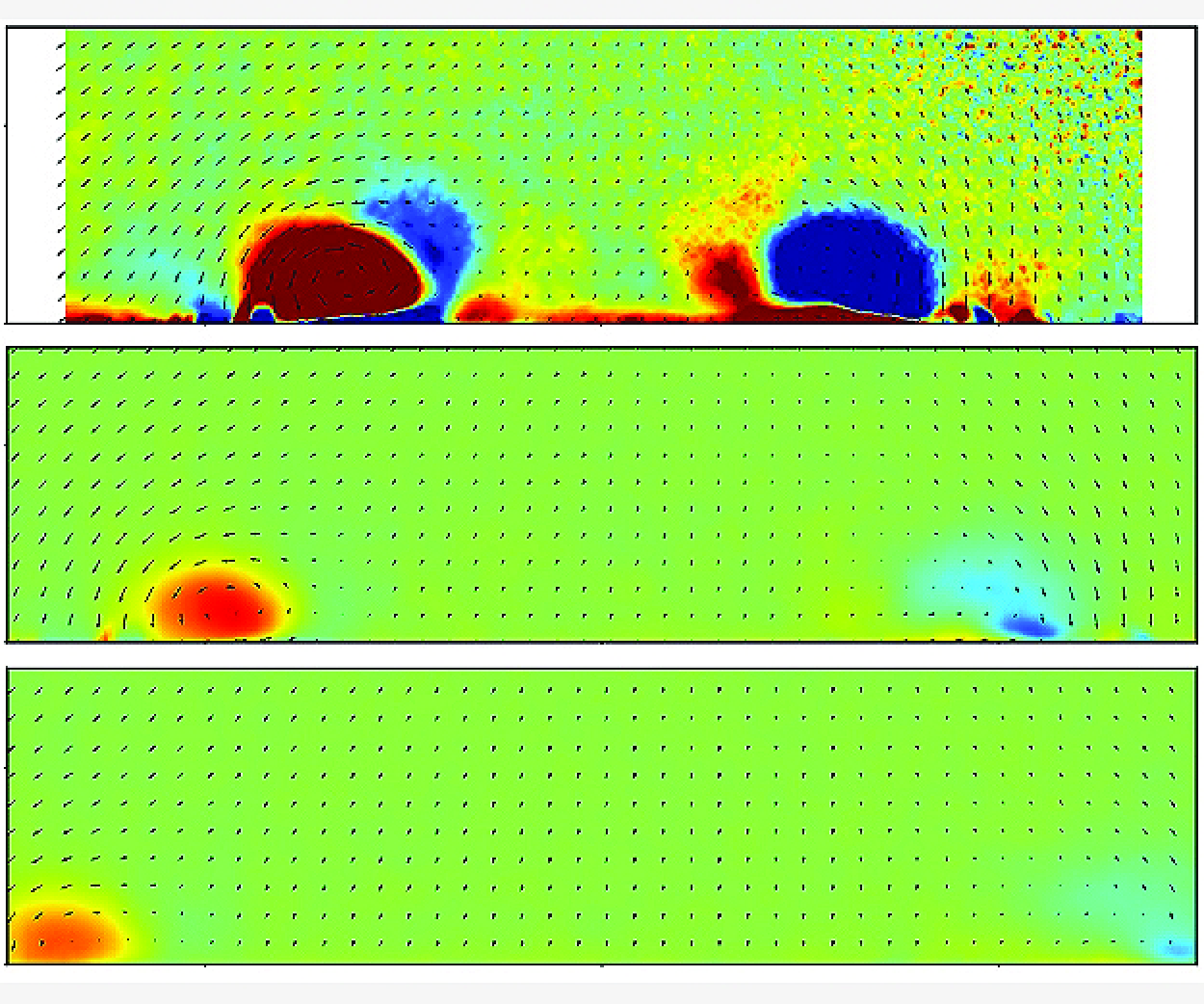
3.2. Plasma-induced flow structure

Each PA generates one pair of counter-rotating streamwise vortices, as is evident in the PIV images (figure 3) captured half-way through the PA array, i.e. $x = -105$ mm (figure 1 b). At $Re_\tau$ = 564 or $x^+= -741$ , the maximum vorticity ${\lvert {\overline {\omega _x^+}}\rvert }_{max}$ is approximately 0.42. However, at $Re_\tau$ = 685 or $x = -1032$ and $Re_\tau$ = 811 or $x^+ = -1352$ , ${\lvert {\overline {\omega _x^+}}\rvert }_{max}$ drops to only 0.24 and 0.18, respectively. The PGSVs at $Re_\tau$ = 564 appear strong, as manifested by their size and vorticity concentration, thus inducing oppositely signed vorticity concentrations around them. This phenomenon is not evident at the higher $Re_\tau$ when the PGSVs weaken in strength (figure 3 $b{,}c$ ). This weakened strength at higher $Re_\tau$ is internally consistent with a decrease in DR with increasing $Re_\tau$ (figure 2 $a{,}b$ ). Note that the cross-sectional area $L^+ \times Re_\tau$ = $L^+ \times {\delta }^+$ of the TBL gradually grows with increasing $Re_\tau$ , implying that the area under the influence of PGSVs contracts at a higher $L^+$ or $Re_\tau$ , with respect to the cross-sectional area of the TBL, which also accounts for the diminished effect of PGSVs and the decreased DR for higher $L^+$ or $Re_\tau$ (figure 2 $c{,}d$ ).

Figure 3. Time-averaged velocity vectors ( $\overline {V^+}$ , $\overline {W^+}$ ) and isocontours of vorticity $\overline {\omega _x^+}$ $\overline {\omega _x^+} = \overline {\textrm {d} V^+ / \textrm {d} z^+} - \overline {\textrm {d} W^+ / \textrm {d} y^+}$ $\overline {\textrm {d} W^+ / \textrm {d} y^+}$ in the $y$ – $z$ plane at the centre ( $x = -105$ mm) of the PA array. Here (a) $Re_\tau$ = 564, (b) 658 and (c) 811. The applied voltage on PAs is 6.0 kV $_{\textrm {p-p}}$ .

4. Theoretical consideration

Vorticity concentrations, as seen in figure 3, originate from the surface of the flat plate, moving with respect to fluid, under the viscosity effect and the no-slip condition (Wu & Wu Reference Wu and Wu1996). In this section, we attempt to understand the generation of skin-friction drag and its reduction based on vorticity dynamics on the boundary between the solid surface and fluid.

On a surface $S$ with unit normal vector $\boldsymbol {n}$ , either inside the fluid or on the boundary, the surface stress may be given following a triple decomposition by

(4.1) \begin{equation} \boldsymbol {t} \equiv \boldsymbol {n} \boldsymbol {\cdot } \boldsymbol {T} = -{\Pi } \boldsymbol {n} + \boldsymbol {\tau } + \boldsymbol {t_s}, \end{equation}

where $\boldsymbol {T}$ is the stress tensor. The terms on the right-hand side of (4.1) are the normal stress, shear stress and surface-deformation stress, respectively, from left to right, and may be written as

(4.2a) \begin{align} -{\Pi }\! \boldsymbol {n} &= -[p-(\lambda +2\mu ) \boldsymbol {\nabla } \boldsymbol {\cdot } \boldsymbol {u}]\boldsymbol {n}, \end{align}

(4.2b) \begin{align} \boldsymbol {\tau } &= \mu \boldsymbol {\omega } \times \boldsymbol {n}, \end{align}

(4.2c) \begin{align} \boldsymbol {t_s} &= -2 \mu \boldsymbol {n} \boldsymbol {\cdot } [(\boldsymbol {\nabla } \boldsymbol {\cdot } \boldsymbol {u}) \boldsymbol {I} -\boldsymbol {\nabla }{\boldsymbol {u}}^T], \end{align}

where $p$ is the pressure, $\lambda$ is the second dynamic viscosity that can be dropped out from the equation for an incompressible fluid, $\mu$ is dynamic viscosity, $\boldsymbol {u}$ is the flow velocity vector, ${\boldsymbol {u}}^T$ is the transpose of $\boldsymbol {u}$ , $\boldsymbol {\nabla }$ is the differential operator, $\boldsymbol {\omega } = \boldsymbol {\nabla } \times \boldsymbol {u}$ is the vorticity vector and $\boldsymbol {I}$ is the unit tensor. Following the Stokes–Helmholtz decomposition, the divergence of $\boldsymbol {T}$ in (4.1) is given by

(4.3) \begin{equation} \boldsymbol {\nabla } \boldsymbol {\cdot } \boldsymbol {T} = -\boldsymbol {\nabla }{\Pi } - \mu (\boldsymbol {\nabla } \times \boldsymbol {\omega }), \end{equation}

where the first and second terms on the right-hand side represent the compression and shear variation, respectively. Taking the curl of (4.3) and applying the continuity equation, we may obtain the following vorticity equation:

(4.4) \begin{equation} \rho \frac {\mathrm {D}}{\mathrm {D}t}\left(\frac {\boldsymbol {\omega }}{\rho }\right) = \boldsymbol {\omega } \boldsymbol {\cdot } \boldsymbol {\nabla }\boldsymbol {u} + \boldsymbol {\nabla } \times \boldsymbol {f} + \frac {1}{{\rho }^2}\boldsymbol {\nabla }\rho \times \boldsymbol {\nabla }{\Pi } - \frac {\mu }{\rho }\boldsymbol {\nabla } \times (\boldsymbol {\nabla } \times \boldsymbol {\omega }), \end{equation}

where $\rho$ is the density of fluid. Thus, the total vorticity variation in a control volume $V$ bounded by $S$ is given by

(4.5) \begin{align} \int _{V}\frac {\mathrm {D}\boldsymbol {\omega }}{\mathrm {D}t}\mathrm {d}V &= \frac {\mathrm {d}}{\mathrm {d}t}\int _{V}\boldsymbol {\omega }\mathrm {d}V \nonumber \\ &= \int _{V}\left(\boldsymbol {\omega } \boldsymbol {\cdot } \boldsymbol {\nabla }\boldsymbol {u} + \frac {1}{{\rho }^2}\boldsymbol {\nabla }\rho \times \boldsymbol {\nabla }{\Pi }\right)\mathrm {d}V + \oint _{S}\boldsymbol {n} \times \boldsymbol {f}\mathrm {d}S - \oint _{S}\upsilon \boldsymbol {n} \times (\boldsymbol {\nabla } \times \boldsymbol {\omega })\mathrm {d}S. \end{align}

The volume integral on the right-hand side of (4.5) includes contributions from vorticity stretching and turning and the baroclinicity, and the first surface integral is due to a non-conservative force $\boldsymbol {f}$ . The integrand of the second surface integral is the boundary vorticity flux (BVF) (Lyman Reference Lyman1990). Using the vector identity, the volume integral of $\boldsymbol {\omega }$ can be expressed in terms of the tangential velocity along the boundary, yielding

(4.6) \begin{equation} \boldsymbol {\mathit {\Gamma }} = \int _{V}\boldsymbol {\omega }\mathrm {d}V = \int _{V}\boldsymbol {\nabla } \times \boldsymbol {u}\mathrm {d}V= \oint _{S} \boldsymbol {n} \times \boldsymbol {u}\mathrm {d}S, \end{equation}

where $\boldsymbol {\mathit {\Gamma }}$ is the vector circulation (Terrington et al. Reference Terrington, Hourigan and Thompson2022; Wu & Wu Reference Wu and Wu1996). Then, on substitution of (4.6) into (4.5), we obtain the following equation:

(4.7) \begin{equation} \frac {\mathrm {d}\boldsymbol {\mathit {\Gamma }}}{\mathrm {d}t} = \int _{V}\left(\boldsymbol {\omega } \boldsymbol {\cdot } \boldsymbol {\nabla }\boldsymbol {u} + \frac {1}{{\rho }^2}\boldsymbol {\nabla }\rho \times \boldsymbol {\nabla }{\Pi }\right)\mathrm {d}V + \oint _{S}\boldsymbol {n} \times \boldsymbol {f}\mathrm {d}S - \oint _{S}\upsilon \boldsymbol {n} \times (\boldsymbol {\nabla } \times \boldsymbol {\omega })\mathrm {d}S. \end{equation}

The BVF in (4.7) represents a transfer of circulation due to the tangential viscous acceleration of fluid on the boundary between two adjacent volumes. Based on Newton’s Second Law, the flow tangential acceleration is directly connected to the force associated with the wall shear stress. Since the wall shear stress in (4.2b) originates from the generation of vorticity, the BVF can be regarded as the origin of skin friction in a TBL (Wang et al. Reference Wang, Eyink and Zaki2022). As such, of particular interest is the change of the viscous term in (4.7), which should be linked directly to a variation in skin friction, say, under control, viz.

(4.8) \begin{equation} \boldsymbol {\Delta F} = \boldsymbol { F_{on}} - \boldsymbol {F_{off}} = g(\boldsymbol {\mathit {\Gamma ^{\prime}}}), \end{equation}

where $\boldsymbol {\mathit {\Gamma ^{\prime}}} = [\oint _{S}\upsilon \boldsymbol {n} \times (\boldsymbol {\nabla } \times \boldsymbol {\omega })\mathrm {d}S]_{on} - [\oint _{S}\upsilon \boldsymbol {n} \times (\boldsymbol {\nabla } \times \boldsymbol {\omega })\mathrm {d}S]_{off}$ .

Under the present plasma control, the vorticity vector $\boldsymbol {\omega } = [\omega _x, \omega _y, \omega _z]$ is predominantly along the streamwise direction due to the generation of PGSVs, and $\omega _y$ and $\omega _z$ are both negligibly small, compared with $\omega _x$ , within the control volume dominated by PGSVs. That is, the vorticity vector can be written as $\boldsymbol {\omega } \approx [\omega _x, 0, 0]$ . Assuming vorticity is conserved, the change in the BVF over the closed control surface which should be adequately large to enclose all the boundary vorticity flux generated by the PA, as given in (4.8), may be estimated approximately by the integral of $\omega _x$ in the $y$ – $z$ plane largely associated with the PGSV, viz.

(4.9) \begin{equation} \mathit {\Gamma ^{\prime}} \approx \oint _{S_p}\omega _x\mathrm {d}y\mathrm {d}z, \end{equation}

where $S_p$ is the surface in the $y$ – $z$ plane where the PGSVs may be adequately captured. The term on the right-hand side of (4.9) is the circulation or strength of PGSVs and can be determined from the PIV data measured in the $y$ – $z$ plane. In view of the limited PIV-measurement resolution, we introduce a threshold $r$ that determines the border of the PGSVs, i.e. ${\lvert {\overline {\omega _x^+}}\rvert } \gt r{\lvert {\overline {\omega _x^+}}\rvert }_{max}$ within the PGSV. Then the wall-unit normalized circulation of the PGSVs can be written as

(4.10) \begin{equation} \mathit {\Gamma ^{\prime}}^{+} _{r} \approx \oint _{S_r}\omega _x^+\mathrm {d}y^+\mathrm {d}z^+, \end{equation}

where $S_r$ is the size of the PGSV.

5. Scaling of DR

Theoretical analysis leads to a finding that the DR depends on only one physical quantity, namely, the variation in the summation of vorticity or circulation within the control volume (4.8). Under control, this variation in circulation is ascribed to the presence of PGSVs (4.9), i.e. due to the artificially generated circulation (4.9) associated with PGSVs. This finding points to the fact that $\Delta F = g_1 (\overline {W}_{max}^+, L^+, {Re_\tau })$ , as observed from figure 2, may be reduced to $\Delta F = g_2 (\xi )$ . However, $g_1$ is an unknown function; it is also a challenge to determine the function $g_2$ and the scaling factor $\xi$ . Fortunately, we have a great amount of experimental data from a physical system. After careful analysis of the experimental data and numerous trial-and-error attempts, we eventually find that $\Delta F = -3.8 \times 10^4 \xi$ (figure 4), where

(5.1) \begin{equation} \xi = \frac {k_{2}\log _{10}{\big(k_{1}\overline {W}_{max}^+\big)}}{L^+ Re_{\tau }} = \frac {k_{2}\log _{10}{\big(k_{1}\overline {W}_{max}^+\big)}}{L^+ {\delta }^+}. \end{equation}

Note that the flow field of the predominantly two-dimensional vortex may be decomposed into the radial and tangential motions, and the vortex strength (or circulation) and the maximum tangential velocity are statistically linked to each other (e.g. Zhou & Antonia Reference Zhou and Antonia1993). Furthermore, the spanwise motion and $\overline {W}_{max}^+$ originate largely from PGSVs. Then, it seems plausible that the numerator of (5.1) is connected to the circulation of PGSVs, and $\xi$ may be interpreted as the circulation per unit area or strength of PGSVs. Interestingly, Thomas et al.’s (Reference Thomas, Corke, Duong, Midya and Yates2019) data also collapse quite well about this line provided $k_1 = 10^3$ and $k_2 \approx 15$ . Furthermore, we may estimate ${\mathit {\Gamma }^{\prime}}^{+} _{r}$ ( $r = 0.1$ ) from the PIV data measured at three Reynolds numbers discussed in §3.2. In the calculation of ${\mathit {\Gamma }^{\prime}}^{+} _{r}$ , we use the absolute values of $\omega _x^+$ to avoid the cancellation of oppositely signed vorticity values associated with the counter-rotating PGSVs. Surprisingly, the dependence of $\Delta F$ on ${\mathit {\Gamma }^{\prime}}^{+} _{r}$ also collapses well about this line once the value of ${\mathit {\Gamma }^{\prime}}^{+} _{r}$ is scaled down by a factor of $2.5 \times 10^{-8}$ , i.e. $2.5 \times 10^{-8} {\mathit {\Gamma }^{\prime}}^{+} _{r}$ . That is, $\Delta F = g_1 (\overline {W}_{max}^+, L^+, {Re_\tau })$ can be also reduced to $\Delta F = g_2 (2.5 \times 10^{-8} {\mathit {\Gamma }^{\prime}}^{+} _{r})$ . All the results demonstrate the reliability and robustness of the scaling law (5.1). The empirical data analysis again demonstrates unequivocally that the DR is proportional to the strength of PGSVs. Clearly, $\Delta F$ drops or DR increases almost linearly with growing $\xi$ . Note that the $Re_{\tau }$ effect is embedded in $\overline {W}_{max}^+$ and $L^+$ because the two parameters are both normalized by wall units that are directly related to $Re_{\tau }$ .

Some remarks are due on the scaling law. In the present study, a sine-AC actuation signal was used, while Thomas et al. (Reference Thomas, Corke, Duong, Midya and Yates2019) deployed pulsed-DC actuation. The latter can generate a much higher instantaneous plasma-induced spanwise wall-jet velocity, compared with the sine-AC actuation, and hence a higher value of $k_2$ . Furthermore, the present PAs generate counter-rotating streamwise vortices, whereas Thomas et al. (Reference Thomas, Corke, Duong, Midya and Yates2019) produced co-rotating streamwise vortices. This difference may also account for the different $k_2$ values in (5.1) or figure 4 between the two studies. It is worth commenting on the departure of experimental data from $\Delta F = -3.8 \times 10^4 \xi$ at large $\xi$ (figure 4). Two factors may contribute to this departure. Firstly, the vortex strength grows with increasing $E_{p{-}p}$ . So does $\xi$ . Beyond a certain level of $E_{p{-}p}$ , the vortices grow in strength rapidly, causing a rise in vortex-induced drag in the TBL (Schoppa & Hussain Reference Schoppa and Hussain1998; Iuso et al. Reference Iuso, Onorato, Spazzini and Cicca2002). Secondly, the large vortex strength at large $\xi$ implies enhanced interactions between neighbouring PGSVs and hence the cancellation effect becomes more appreciable. Both factors cause experimental data below the fitting curve. It is worth commenting on the large departure of two data points (marked by dashed circles), extracted from Thomas et al. (Reference Thomas, Corke, Duong, Midya and Yates2019), from the scaling law in figure 4. These points were obtained at relatively low $Re_{\tau }$ and showed appreciable deviation from their other data (their figure 15). This deviation arises from a limited resolution, approximately 0.04 g, in their force balance, which is inadequate to capture a very small skin-friction drag of 0.029 g at $Re_{\tau } = 1937$ (Thomas et al. Reference Thomas, Corke, Duong, Midya and Yates2019).

Figure 4. Dependence of drag variation $\Delta F$ on $\xi =[k_{2} \log _{10}(k_{1} \overline {W}_{\max }^{+})] /(L^{+} Re_{\tau })$ , where $k_1 = 10^3$ and $k_2 \approx 1$ for the present results and $k_1 = 10^3$ and $k_2 \approx 15$ for the Thomas et al.’s (Reference Thomas, Corke, Duong, Midya and Yates2019) results. The black cross symbols are $2.5 \times 10^{-8}$ times the measured circulation ${\mathit {\Gamma }^{\prime}}^{+} _{0.1}$ of the PGSV, whose border is defined at ${\lvert {\overline {\omega _x^+}}\rvert } = 0.1{\lvert {\overline {\omega _x^+}}\rvert }_{max}$ ( $E_{p{-}p}$ = 6 kV $_{\textrm {p-p}}$ and $Re_\tau$ = 564, 658 and 811). The large departure of two data points from Thomas et al. (Reference Thomas, Corke, Duong, Midya and Yates2019) are marked by dashed circles. The error bars denote the standard deviation out of 12 repeated measurements.

Several interesting inferences can be made from the scaling law. Firstly, given two of the three parameters $\overline {W}_{max}^+$ , $L^+$ and $Re_{\tau }$ , the dependence of $\Delta F$ on the remaining parameter may be determined from the scaling law. For example, given $L^+$ and $Re_{\tau }$ , $\Delta F$ drops or DR rises logarithmically with increasing $\overline {W}_{max}^+$ , as measurements (figure 2 a) indicate. Evidently, the relationship between $\Delta F$ and $L^+$ or $Re_{\tau }$ derived from the scaling law is also as in figure 2( $b{,}c$ ). With $\Delta F$ and $\overline {W}_{max}^+$ given, we may also determine the relation between $L^+$ and $Re_{\tau }$ . Thus, the scaling law provides a powerful tool for the PA design and also the control performance prediction. Secondly, given $\xi$ or $\Delta F$ , $\overline {W}_{max}^+$ diminishes with decreasing $L^+$ or $Re_{\tau }$ , implying less energy consumption and thus higher control efficiency. Figure 5(a) presents the dependence of $\Delta F$ on $\overline {W}_{max}^+$ and $L^+ Re_{\tau }$ . The control efficiency $\eta = (F_{on} - F_{off})U_{\infty }/P_{input}$ is also given in the figure, as marked by the thick black crosses, where $P_{input}$ is the power consumption determined by the Q–V cycloramas (Lissajous figure) measured through two parallel- and series-connected capacitances at $\Delta F \approx -0.185$ . Evidently, $\eta$ drops with the shrinking $L^+ Re_{\tau }$ and $\overline {W}_{max}^+$ . Thirdly, Thomas et al. (Reference Thomas, Corke, Duong, Midya and Yates2019) proposed $\Delta F = g_3(L^+, \overline {W}_{max}^+)$ , where $g_3$ was a unknown function and the effect of $Re_{\tau}$ on ${\Delta}F$ was not considered. Indeed, the $\Delta F$ – $L^+$ and $\Delta F$ – $Re_{\tau }$ relationships are similar, as shown in figure 2( $c{,}d$ ). In fact, $L^+$ and $Re_{\tau }$ are strictly nonlinear. However, this nonlinearity is very weak. Readers are cautioned that further experiments need to be conducted should this approximate linearity be extended beyond the range of $Re_\tau = 564 \sim 4336$ presently examined. Consequently, $\xi$ can be further simplified to $\xi ^{\prime} = [k_{2} \log _{10} (k_{1} \overline {W}_{max }^{+} ) ] /L^{+}$ (figure 5 b), where $k_1 = 10^4$ and $k_2\approx 1$ for the present data and $k_1 = 10^4$ and $k_2\approx 3$ for Thomas et al.’s (Reference Thomas, Corke, Duong, Midya and Yates2019) data. This simplified equation involves only two parameters, thus facilitating calculation and analysis in predicting DR. The least-squares fitting curve is now given by $\Delta F = g_3 (\xi ^{\prime}) \approx -4300{\xi ^{\prime}}^{2}-6.3\xi ^{\prime} -0.02$ . Note that $2.5 \times 10^{-8} {\mathit {\Gamma }^{\prime}}^{+} _{0.1}$ in figure 4 is now $1.8 \times 10^{-5} {\mathit {\Gamma }^{\prime}}^{+} _{0.1}$ in figure 5(b). Finally, DR can be predicted once $\xi$ or $\xi ^{\prime}$ is known or vice versa. By determining the value of $\xi$ or $\Delta F$ , the magnitudes of the applied voltages can be adjusted precisely in accordance with $Re_{\tau }$ to achieve the optimal plasma-induced velocity, thereby attaining the desired specific DR. This approach also aids in the design of PA arrays, such as the choice of $L$ .

Figure 5. (a) Dependence of $\Delta F$ on $\overline {W}_{max}^+$ and $L^+Re_\tau$ . The control efficiency $\eta$ estimated at $\Delta F \approx -0.185$ is given at three points, marked by black crosses. The dotted lines are the isocontours of $\Delta F$ and the arrow indicates the direction of increasing $\eta$ . (b) Dependence of drag variation $\Delta F$ on $\Delta F$ . The black crosses mark the measured circulation ${\mathit {\Gamma }^{\prime}}^{+} _{0.1} \times 1.8 \times 10^{-5}$ of the PGSV, whose border is defined at ${\lvert {\overline {\omega _x^+}}\rvert } = 0.1{\lvert {\overline {\omega _x^+}}\rvert }_{max}$ . The error bars denote the standard deviation out of 12 repeated measurements.