


1. Introduction
In regions of strong oceanic currents (for example, the Gulf Stream, the Agulhas Current and the Kuroshio Current), exceptionally high waves, also known as freak or rogue waves, may arise as a result of the interaction between waves and the current field (Peregrine Reference Peregrine1976). It is interesting, in this respect, that a number of ship accidents has been reported near the Agulhas Current, off the South African coast (Lavrenov Reference Lavrenov1998; White & Fornberg Reference White and Fornberg1998; Toffoli et al.
Reference Toffoli, Lefèvre, Bitner-Gregersen and Monbaliu2005). In the presence of a background current, wave frequencies undergo a Doppler shift: waves are transported by the current and the resulting phase velocity is the sum of the phase velocity in the absence of current plus the current velocity. For a current variable in space, wave trajectories can also be deviated like electromagnetic waves, which are refracted when encountering a non-homogeneous medium. These effects are well known and documented in classical review papers (e.g. Peregrine Reference Peregrine1976) and books (e.g. Johnson Reference Johnson1997). Depending on the nature of the current, furthermore, wave energy can also be focused in space, leading to the formation of large-amplitude waves (Lavrenov Reference Lavrenov1998; White & Fornberg Reference White and Fornberg1998; Lavrenov & Porubov Reference Lavrenov and Porubov2006). When the velocity of the current is equal to or larger than
 $1/4$
of the wave phase speed (Johnson Reference Johnson1997), currents may also block the propagation of waves. The above effects can be derived in a systematic way from the inviscid and irrotational equations of motion under the linear approximation. However, the relevance of the nonlinear effects in these circumstances is not well understood, mainly because of the analytical difficulties introduced by the nonlinearity itself. In Shrira & Slunyaev (Reference Shrira and Slunyaev2014), the phenomenon of trapping of waves by an opposing jet current has been studied, and the formation of a long-lived structure, stable with respect to transverse perturbations, has been verified numerically. It is argued that such a structure could potentially result in an increase in the probability of formation of rogue waves.
$1/4$
of the wave phase speed (Johnson Reference Johnson1997), currents may also block the propagation of waves. The above effects can be derived in a systematic way from the inviscid and irrotational equations of motion under the linear approximation. However, the relevance of the nonlinear effects in these circumstances is not well understood, mainly because of the analytical difficulties introduced by the nonlinearity itself. In Shrira & Slunyaev (Reference Shrira and Slunyaev2014), the phenomenon of trapping of waves by an opposing jet current has been studied, and the formation of a long-lived structure, stable with respect to transverse perturbations, has been verified numerically. It is argued that such a structure could potentially result in an increase in the probability of formation of rogue waves.
In the absence of a background current, the formation of rogue waves is often attributed to a modulational instability process (e.g. Kharif, Pelinovsky & Slunyaev Reference Kharif, Pelinovsky and Slunyaev2009). This mechanism predicts an exponential growth of small perturbations, when
 ${\it\varepsilon}N\geqslant 1/\sqrt{2}$
, where
${\it\varepsilon}N\geqslant 1/\sqrt{2}$
, where
 ${\it\varepsilon}=ka$
is the steepness of the plane wave, with
${\it\varepsilon}=ka$
is the steepness of the plane wave, with
 $k$
its wavenumber and
$k$
its wavenumber and
 $a$
its amplitude, and
$a$
its amplitude, and
 $N={\it\omega}/{\rm\Delta}{\it\Omega}$
is the number of waves under the modulation, with
$N={\it\omega}/{\rm\Delta}{\it\Omega}$
is the number of waves under the modulation, with
 ${\it\omega}$
the angular frequency corresponding to the wavenumber
${\it\omega}$
the angular frequency corresponding to the wavenumber
 $k$
and
$k$
and
 ${\rm\Delta}{\it\Omega}$
the angular frequency of the modulation (see Zakharov & Ostrovsky Reference Zakharov and Ostrovsky2009, and references therein for an overview). The nonlinear stages of modulational instability are described by exact breather solutions of the nonlinear Schrödinger (NLS) equation (e.g. Akhmediev, Eleonskii & Kulagin Reference Akhmediev, Eleonskii and Kulagin1987), which are coherent structures that oscillate in space or time. Breathers exhibit the remarkable property of changing their amplitudes as they propagate, allowing a growth of up to a maximum of three times their initial amplitude. For this reason, they have been considered as plausible objects to describe the formation of rogue waves (see, e.g., Dysthe & Trulsen Reference Dysthe and Trulsen1999; Osborne, Onorato & Serio Reference Osborne, Onorato and Serio2000; Akhmediev, Soto-Crespo & Ankiewicz Reference Akhmediev, Soto-Crespo and Ankiewicz2009; Shrira & Geogjaev Reference Shrira and Geogjaev2010, among others). Such solutions have been reproduced experimentally in wave tanks, see Chabchoub, Hoffmann & Akhmediev (Reference Chabchoub, Hoffmann and Akhmediev2011) and Chabchoub et al. (Reference Chabchoub, Hoffmann, Onorato, Slunyaev, Sergeeva, Pelinovsky and Akhmediev2012). It should be noted that breathers may also exist embedded in random waves (Onorato et al.
Reference Onorato, Osborne, Serio and Bertone2001) and hence affect the probability density function of the surface elevation and wave height (Onorato et al.
Reference Onorato, Osborne, Serio, Brandini and Stansberg2004; Mori et al.
Reference Mori, Onorato, Janssen, Osborne and Serio2007). Provided that the random wavefield is sufficiently steep and the related spectrum is narrow banded, strong deviations from Gaussian statistics take place (e.g. Janssen Reference Janssen2003; Onorato et al.
Reference Onorato, Cavaleri, Fouques, Gramstad, Janssen, Monbaliu, Osborne, Pakozdi, Serio, Stansberg, Toffoli and Trulsen2009a
,Reference Onorato, Waseda, Toffoli, Cavaleri, Gramstad, Janssen, Kinoshita, Monbaliu, Mori, Osborne, Serio, Stansberg, Tamura and Trulsen
b
; Waseda, Kinoshita & Tamura Reference Waseda, Kinoshita and Tamura2009).
${\rm\Delta}{\it\Omega}$
the angular frequency of the modulation (see Zakharov & Ostrovsky Reference Zakharov and Ostrovsky2009, and references therein for an overview). The nonlinear stages of modulational instability are described by exact breather solutions of the nonlinear Schrödinger (NLS) equation (e.g. Akhmediev, Eleonskii & Kulagin Reference Akhmediev, Eleonskii and Kulagin1987), which are coherent structures that oscillate in space or time. Breathers exhibit the remarkable property of changing their amplitudes as they propagate, allowing a growth of up to a maximum of three times their initial amplitude. For this reason, they have been considered as plausible objects to describe the formation of rogue waves (see, e.g., Dysthe & Trulsen Reference Dysthe and Trulsen1999; Osborne, Onorato & Serio Reference Osborne, Onorato and Serio2000; Akhmediev, Soto-Crespo & Ankiewicz Reference Akhmediev, Soto-Crespo and Ankiewicz2009; Shrira & Geogjaev Reference Shrira and Geogjaev2010, among others). Such solutions have been reproduced experimentally in wave tanks, see Chabchoub, Hoffmann & Akhmediev (Reference Chabchoub, Hoffmann and Akhmediev2011) and Chabchoub et al. (Reference Chabchoub, Hoffmann, Onorato, Slunyaev, Sergeeva, Pelinovsky and Akhmediev2012). It should be noted that breathers may also exist embedded in random waves (Onorato et al.
Reference Onorato, Osborne, Serio and Bertone2001) and hence affect the probability density function of the surface elevation and wave height (Onorato et al.
Reference Onorato, Osborne, Serio, Brandini and Stansberg2004; Mori et al.
Reference Mori, Onorato, Janssen, Osborne and Serio2007). Provided that the random wavefield is sufficiently steep and the related spectrum is narrow banded, strong deviations from Gaussian statistics take place (e.g. Janssen Reference Janssen2003; Onorato et al.
Reference Onorato, Cavaleri, Fouques, Gramstad, Janssen, Monbaliu, Osborne, Pakozdi, Serio, Stansberg, Toffoli and Trulsen2009a
,Reference Onorato, Waseda, Toffoli, Cavaleri, Gramstad, Janssen, Kinoshita, Monbaliu, Mori, Osborne, Serio, Stansberg, Tamura and Trulsen
b
; Waseda, Kinoshita & Tamura Reference Waseda, Kinoshita and Tamura2009).
When propagating over a current with adverse gradients in the horizontal velocity (i.e. an accelerating opposing current or a decelerating following current), waves undergo a transformation that shortens the wavelength and increases the wave height (Longuet-Higgins & Stewart Reference Longuet-Higgins and Stewart1961; Peregrine Reference Peregrine1976). As a result, the waves become steeper, amplifying nonlinear processes (see, e.g., Smith Reference Smith1976; Gerber Reference Gerber1987; Lai, Long & Huang Reference Lai, Long and Huang1989; Chawla Reference Chawla2000). Therefore, an initial wave whose perturbation is stable (or weakly unstable) in terms of the modulational instability may become strongly unstable. This may consequently trigger the formation of breathers in the presence of a current, because of a shift of the modulational instability band. This conjecture has been foreshadowed in a number of theoretical, numerical and experimental studies over recent decades (see, for example, Gerber Reference Gerber1987; Lai et al.
Reference Lai, Long and Huang1989; Stocker & Peregrine Reference Stocker and Peregrine1999; Chawla Reference Chawla2000; Chawla & Kirby Reference Chawla and Kirby2002; Suastika Reference Suastika2004; Ma et al.
Reference Ma, Dong, Perlin, Ma, Wang and Xu2010; Toffoli et al.
Reference Toffoli, Cavaleri, Babanin, Benoit, Bitner-Gregersen, Monbaliu, Onorato, Osborne and Stansberg2011; Moreira & Peregrine Reference Moreira and Peregrine2012, among others). Only recently, however, has the amplification of wave instability induced by adverse current gradients and the concurrent generation of extremes been confirmed theoretically (Hjelmervik & Trulsen Reference Hjelmervik and Trulsen2009; Onorato, Proment & Toffoli Reference Onorato, Proment and Toffoli2011; Ruban Reference Ruban2012) and experimentally (Ma et al.
Reference Ma, Ma, Perlin and Dong2013; Toffoli et al.
Reference Toffoli, Waseda, Houtani, Kinoshita, Collins, Proment and Onorato2013). In this regard, results have substantiated that the envelope of an initially weakly unstable regular wave train begins to be strongly modulated, after an initial growth in amplitude of the whole envelope, when it enters into a region of strong opposing current. The maximum amplitude grows for increasing current gradients in the form of the ratio
 $U/c_{g}$
, where
$U/c_{g}$
, where
 $U$
is the current speed and
$U$
is the current speed and
 $c_{g}$
is the wave group velocity. Experimental records of amplitude growth as a function of
$c_{g}$
is the wave group velocity. Experimental records of amplitude growth as a function of
 $U/c_{g}$
appeared to be in reasonable agreement with predictions based on a current-modified NLS equation in Ruban (Reference Ruban2012) and Toffoli et al. (Reference Toffoli, Waseda, Houtani, Kinoshita, Collins, Proment and Onorato2013) (see, for example, figure 3 in Toffoli et al.
Reference Toffoli, Waseda, Houtani, Kinoshita, Collins, Proment and Onorato2013). Opposing shear currents can also modify the modulational instability. Such an issue has been recently addressed in Thomas, Kharif & Manna (Reference Thomas, Kharif and Manna2012), where it has been shown that the result is independent of the non-dimensional water depth.
$U/c_{g}$
appeared to be in reasonable agreement with predictions based on a current-modified NLS equation in Ruban (Reference Ruban2012) and Toffoli et al. (Reference Toffoli, Waseda, Houtani, Kinoshita, Collins, Proment and Onorato2013) (see, for example, figure 3 in Toffoli et al.
Reference Toffoli, Waseda, Houtani, Kinoshita, Collins, Proment and Onorato2013). Opposing shear currents can also modify the modulational instability. Such an issue has been recently addressed in Thomas, Kharif & Manna (Reference Thomas, Kharif and Manna2012), where it has been shown that the result is independent of the non-dimensional water depth.
At present, results are limited to the evolution of regular wavepackets. Despite some attempts with irregular wavefields (e.g. Toffoli et al. Reference Toffoli, Cavaleri, Babanin, Benoit, Bitner-Gregersen, Monbaliu, Onorato, Osborne and Stansberg2011), it is not clear yet whether, and to what extent, this current-induced destabilisation affects wave amplitude growth and the probability of extremes in more realistic random wavefields. The occurrence of breaking dissipation as a result of wave steepening also adds to this uncertainty. Here, the dynamics of random waves on adverse current gradients is assessed experimentally in three independent facilities: the wave flume and the ocean wave basin at the Coastal, Ocean and Sediment Transport (COAST) Laboratory of Plymouth University and the Ocean Engineering Tank of the University of Tokyo. In all facilities, experiments consisted of monitoring the evolution of mechanically generated waves, when propagating against opposing currents of variable speeds (ranging from a very mild current to a speed approaching the blocking limit). Whereas the wave flume only allows the investigation of unidirectional wavefields, wave basins permit the evolution of both unidirectional and directional waves to be traced. A detailed description of the experiments is presented in §§ 2 and 3. In § 4, the amplification of modulational instability in weakly unstable regular wavepackets due to an adverse current is briefly discussed to verify that the underlying physics occurs in all facilities. The role of breaking on amplitude growth is also discussed. The effect of an opposing current on nonlinear properties and the occurrence of extremes in random unidirectional and directional wavefields is demonstrated in § 5. Specifically, experimental records corroborate in a robust and consistent manner that unidirectional wavefields undergo a transformation from weakly to strongly non-Gaussian properties when interacting with an opposing current gradient. This transition depends directly on the intensity of the current gradient. To a certain extent, this also applies in directional sea states, where the occurrence of rogue waves is least expected.
2. Laboratory experiments and facilities
2.1. Experimental model
The experiment consisted of monitoring the evolution of regular and irregular waves, when entering into a region of opposing current. Tests were carried out in two independent ocean basins, one at Plymouth University and one at the University of Tokyo, where propagation in two horizontal dimensions is permitted. Both unidirectional and more realistic directional wavefields were investigated. An experiment was also undertaken in the wave flume at Plymouth University, where only unidirectional propagation is allowed, to provide data for a further independent verification of the results. The facilities are schematised in figure 1.

Figure 1. Schematic representation of the facilities: (a) wave flume at Plymouth University; (b) wave basin at Plymouth University; (c) wave basin at University of Tokyo.
Waves were mechanically generated by imposing an input spectrum at the wavemaker. Overall, wave steepness was kept sufficiently small to maintain a weakly unstable condition and thus avoid the development of modulational instability within the boundaries of the facilities in the absence of a background current. The conversion from spectral energy to voltage was carried out by an inverse fast Fourier transform with random amplitude and random phase approximation (cf. Onorato et al. Reference Onorato, Cavaleri, Fouques, Gramstad, Janssen, Monbaliu, Osborne, Pakozdi, Serio, Stansberg, Toffoli and Trulsen2009a , for example). The current was imposed by recirculating water flow through the basin in the direction opposite to the waves.
2.2. Wave flume at Plymouth University
The wave flume at the COAST Laboratory of Plymouth University is 35 m long and 0.6 m wide, with a uniform water depth (
 $d$
) of 0.75 m. The facility is equipped with a piston wavemaker with active force absorption at one end and a passive absorber panel at the other end. We remark that only unidirectional propagation is allowed in this facility. The flume is also equipped with a pump for the generation of a background current of up to
$d$
) of 0.75 m. The facility is equipped with a piston wavemaker with active force absorption at one end and a passive absorber panel at the other end. We remark that only unidirectional propagation is allowed in this facility. The flume is also equipped with a pump for the generation of a background current of up to
 $0.5~\text{m}~\text{s}^{-1}$
, which can follow or oppose the wave direction of propagation (but only an opposing current was used for the present study). Either the inlet or the outlet is located near the absorber, while the other is at a distance of approximately 2.5 m from the wavemaker (see figure 1
a). This particular configuration allows waves to be generated outside the current field and propagate for a few wavelengths before encountering a current gradient.
$0.5~\text{m}~\text{s}^{-1}$
, which can follow or oppose the wave direction of propagation (but only an opposing current was used for the present study). Either the inlet or the outlet is located near the absorber, while the other is at a distance of approximately 2.5 m from the wavemaker (see figure 1
a). This particular configuration allows waves to be generated outside the current field and propagate for a few wavelengths before encountering a current gradient.
The wavefield was monitored with 10 capacitance wave gauges equally spaced along the flume, while the velocity field was monitored with two properly seeded acoustic Doppler velocimeters (ADVs). All instrumentation was operated at a sampling frequency of 128 Hz.
A survey of the current was conducted by measuring 10 min series at different locations. The results revealed a fairly uniform flow both longitudinally and transversely. Averaged profiles are presented in figure 2(a–c). Over the entire time series, the standard deviation was approximately 10 % (with peaks at high current speeds), and temporal variations occurred within a period of approximately 10 s.

Figure 2. Longitudinal, transverse and vertical profiles of the horizontal current velocity for (a–c) the wave flume at Plymouth University, (d–f) the wave basin at Plymouth University and (g–i) the wave basin at the University of Tokyo.
2.3. Wave basin at Plymouth University
The ocean wave basin at the COAST Laboratory of Plymouth University is 35 m long and 15.5 m wide. The floor is movable and it was set to a depth of 3 m for the present experiment. The facility allows propagation in two horizontal dimensions and it is equipped with 24 individually controlled wave paddles. At the other end, a convex beach is installed for wave energy absorption. A background current is forced by a multipump recirculating hydraulic system, which is capable of producing a water flow with speed (
 $U$
) ranging from 0.03 to
$U$
) ranging from 0.03 to
 $0.4~\text{m}~\text{s}^{-1}$
(both following and opposing the waves). The inlet and outlet are located on the floor just in front of the wave pistons and the beach. For an opposing current (i.e. propagating against the waves), the particular location of the outlet ensures a gradual deceleration of surface velocity, while approaching the wavemaker. This, in turn, ensures that waves are subjected to an adverse current gradient immediately after being generated.
$0.4~\text{m}~\text{s}^{-1}$
(both following and opposing the waves). The inlet and outlet are located on the floor just in front of the wave pistons and the beach. For an opposing current (i.e. propagating against the waves), the particular location of the outlet ensures a gradual deceleration of surface velocity, while approaching the wavemaker. This, in turn, ensures that waves are subjected to an adverse current gradient immediately after being generated.
The evolution of the surface elevation was traced by 10 capacitance wave gauges deployed at an interval of 2.5 m, starting from the wavemaker and approximately 2.5 m from the (left) sidewall. Probes were operated at a sampling frequency of 128 Hz.
A propeller current meter was used to monitor the average current velocity (the instrument already provided an averaged current speed over a minute). The longitudinal, transverse and vertical profiles of the horizontal velocity are presented in figure 2(d–f). The records indicate a sharp gradient from
 $0~\text{m}~\text{s}^{-1}$
to the regime speed within the first 2 m of wave propagation. Towards the middle of the basin, there is a slight deceleration (between 2 and 10 m from the wavemaker), while the current sharply accelerates in the proximity of the centre (see figure 2
d). Transversely, the current remains stable. A 10 min time series of velocity was gathered to monitor temporal oscillations with a properly seeded ADV. Over time, the standard deviation was approximately 15 % due to long-period oscillations of approximately 80 s.
$0~\text{m}~\text{s}^{-1}$
to the regime speed within the first 2 m of wave propagation. Towards the middle of the basin, there is a slight deceleration (between 2 and 10 m from the wavemaker), while the current sharply accelerates in the proximity of the centre (see figure 2
d). Transversely, the current remains stable. A 10 min time series of velocity was gathered to monitor temporal oscillations with a properly seeded ADV. Over time, the standard deviation was approximately 15 % due to long-period oscillations of approximately 80 s.
2.4. Wave basin at the University of Tokyo
The Ocean Engineering Tank of the Institute of Industrial Science, University of Tokyo (Kinoshita Laboratory and Rheem Laboratory) is 50 m long, 10 m wide and 5 m deep. It is equipped with a multidirectional wavemaker with 32 triangular plungers, which are digitally controlled to generate regular and irregular waves of various periods between 0.5 and 5 s and propagating at prescribed angles (see Waseda et al.
Reference Waseda, Kinoshita and Tamura2009, for more details). A sloping beach is deployed opposite the wavemaker to absorb the wave energy. The tank is also equipped with a pump (located beside the basin) for the generation of background currents, which can follow or oppose the waves. Either the inlet or the outlet is located on the vertical wall just below the beach, while the other is located just below the wavemaker. For waves opposing the current, the flow speed at the surface is thus expected to decelerate near the wavemaker. This ensures that waves undergo an adverse current gradient immediately after generation. Flow velocities can be selected from a minimum of
 $0.02~\text{m}~\text{s}^{-1}$
up to a maximum of approximately
$0.02~\text{m}~\text{s}^{-1}$
up to a maximum of approximately
 $0.4~\text{m}~\text{s}^{-1}$
. It should be noted that no modification of the cross section was performed locally to modify the velocity field.
$0.4~\text{m}~\text{s}^{-1}$
. It should be noted that no modification of the cross section was performed locally to modify the velocity field.
Wave probes were deployed along the tank at a distance of 2.5 m from the sidewall and arranged at 5 m intervals to monitor the evolution of wave trains. At approximately 27 m from the wavemaker, an array of six probes configured as a pentagon with one probe at the centre of gravity was installed to monitor directional properties. Probes were operated at a sampling frequency of 100 Hz.
Two electromagnetic velocimeters were used to survey the current. Instruments were deployed at several locations in the tank and at a depth of 0.2 m. Velocity measurements were also gathered at a sampling frequency of 100 Hz; a 10 s moving average filter was applied to smooth the signal. Instantaneous measurements of horizontal velocity revealed a substantial spatial and temporal speed variation along the tank, with a dominant oscillation period of approximately 150 s. Average values over the measured 10 min series are presented in figure 2(g–i). It should be noted that the standard deviation is approximately 25 % of the mean over the entire time series. As the flow outlet is located just below the wave generator, the velocity is approximately zero at a distance of approximately 0.2 m from the wavemaker, while the flow is in a regime at a distance of 5 m from the wavemaker. Waves are therefore generated in a condition of (almost) still water and enter into an opposing current approximately 1 m after being generated. Farther from the wavemaker, between 5 and 30 m from the generator, the current still shows a weak gradient, which may slightly affect the wavefield. It should be noted that the average horizontal velocity weakly decreased with the water depth: on average, the vertical gradient was approximately 2 %
 $\text{m}^{-1}$
.
$\text{m}^{-1}$
.
Interestingly enough, the survey of the current field also indicates that the stream runs faster on the left-hand side (with respect to the mean wave direction of propagation and along the line of deployment of wave probes), while it is slower on the other side. A flow straightener, in this respect, was not applied during the experiments. Although this difference is negligible for slow currents, it generates a substantial refraction when the current speed is rather high (see figure 3). As a result, waves are redirected towards the sidewall. This may potentially enhance wave amplitude growth as a result of linear directional focusing and hence increase breaking probability.

Figure 3. Current-induced refraction in the basin at the University of Tokyo.
3. Initial conditions
3.1. Regular wavepackets
Test were conducted to trace the evolution of marginally unstable regular wavepackets to sideband perturbations. The initial signal at the wavemaker consisted of a three-component system: a carrier wave and two (i.e. lower and upper) sidebands. Experiments in the wave flume at Plymouth University and in the wave basin at the University of Tokyo were undertaken with a carrier wave of period
 $T_{0}=0.8~\text{s}$
(wavelength
$T_{0}=0.8~\text{s}$
(wavelength
 ${\it\lambda}_{0}=2{\rm\pi}/k_{0}\simeq 1~\text{m}$
), while the dominant wave period was set to
${\it\lambda}_{0}=2{\rm\pi}/k_{0}\simeq 1~\text{m}$
), while the dominant wave period was set to
 $T_{0}=0.7~\text{s}$
(
$T_{0}=0.7~\text{s}$
(
 ${\it\lambda}_{0}=0.76~\text{m}$
) in the basin at Plymouth University. It should be noted that these periods/wavelengths ensure a space scale for wave evolution of at least 30 wavelengths in all facilities. The two sidebands were defined with amplitudes
${\it\lambda}_{0}=0.76~\text{m}$
) in the basin at Plymouth University. It should be noted that these periods/wavelengths ensure a space scale for wave evolution of at least 30 wavelengths in all facilities. The two sidebands were defined with amplitudes
 $b_{\pm }$
equal to 0.25 times the amplitude
$b_{\pm }$
equal to 0.25 times the amplitude
 $a_{c}$
of the carrier wave. This forces the wavepacket to start at an advanced stage of the modulation so that instability can occur within the tanks (Tulin & Waseda Reference Tulin and Waseda1999; Waseda et al.
Reference Waseda, Rheem, Sawamura, Yuhara, Kinoshita, Tanizawa and Tomita2005). The dominant (carrier) component was defined in such a way that the wave steepness was
$a_{c}$
of the carrier wave. This forces the wavepacket to start at an advanced stage of the modulation so that instability can occur within the tanks (Tulin & Waseda Reference Tulin and Waseda1999; Waseda et al.
Reference Waseda, Rheem, Sawamura, Yuhara, Kinoshita, Tanizawa and Tomita2005). The dominant (carrier) component was defined in such a way that the wave steepness was
 $k_{0}a_{0}=0.064$
with
$k_{0}a_{0}=0.064$
with
 $a_{0}^{2}=a_{c}^{2}+b_{+}^{2}+b_{-}^{2}$
. The frequency of the disturbances was chosen to force the number of waves under the perturbation
$a_{0}^{2}=a_{c}^{2}+b_{+}^{2}+b_{-}^{2}$
. The frequency of the disturbances was chosen to force the number of waves under the perturbation
 $N={\it\omega}_{0}/{\rm\Delta}{\it\Omega}$
(with
$N={\it\omega}_{0}/{\rm\Delta}{\it\Omega}$
(with
 ${\it\omega}_{0}$
being the angular frequency of the carrier waves) to be equal to 11. Under these circumstances, the perturbation frequency lies at the edge of the NLS-based instability region, i.e. waves are marginally unstable (
${\it\omega}_{0}$
being the angular frequency of the carrier waves) to be equal to 11. Under these circumstances, the perturbation frequency lies at the edge of the NLS-based instability region, i.e. waves are marginally unstable (
 ${\it\varepsilon}N=k_{0}a_{0}N=0.70\approx 1/\sqrt{2}$
). The evolution of these packets was tested with increasing current velocities up to the blocking conditions (
${\it\varepsilon}N=k_{0}a_{0}N=0.70\approx 1/\sqrt{2}$
). The evolution of these packets was tested with increasing current velocities up to the blocking conditions (
 $U\approx 0.3~\text{m}~\text{s}^{-1}$
).
$U\approx 0.3~\text{m}~\text{s}^{-1}$
).
3.2. Random unidirectional wavefields
Initial conditions for random wavefields were generated using a JONSWAP spectrum (Komen et al.
Reference Komen, Cavaleri, Donelan, Hasselmann, Hasselmann and Janssen1994). In the basin at Plymouth University, the spectral shape was defined by a peak period
 $T_{p}=0.7~\text{s}$
(hence wavelength
$T_{p}=0.7~\text{s}$
(hence wavelength
 $L_{p}=0.765~\text{m}$
, group velocity
$L_{p}=0.765~\text{m}$
, group velocity
 $c_{g}=0.55~\text{m}~\text{s}^{-1}$
and relative water depth
$c_{g}=0.55~\text{m}~\text{s}^{-1}$
and relative water depth
 $k_{p}d=24.6$
), significant wave height
$k_{p}d=24.6$
), significant wave height
 $H_{s}=0.015~\text{m}$
and peak enhancement factor
$H_{s}=0.015~\text{m}$
and peak enhancement factor
 ${\it\gamma}=3$
. The resulting wavefield is characterised by a wave steepness
${\it\gamma}=3$
. The resulting wavefield is characterised by a wave steepness
 $k_{p}H_{s}/2=0.062$
, where
$k_{p}H_{s}/2=0.062$
, where
 $k_{p}$
is the wavenumber associated with the spectral peak. Under these circumstances, the wavefield is expected to remain weakly non-Gaussian in the absence of currents. To set a reference, the evolution of the input wavefield was first traced with no current. Experiments were then repeated with opposing currents at nominal velocities of
$k_{p}$
is the wavenumber associated with the spectral peak. Under these circumstances, the wavefield is expected to remain weakly non-Gaussian in the absence of currents. To set a reference, the evolution of the input wavefield was first traced with no current. Experiments were then repeated with opposing currents at nominal velocities of
 $U=-0.01$
,
$U=-0.01$
,
 $-0.04$
,
$-0.04$
,
 $-0.08$
,
$-0.08$
,
 $-0.11$
,
$-0.11$
,
 $-0.13$
,
$-0.13$
,
 $-0.15$
and
$-0.15$
and
 $-0.19~\text{m}~\text{s}^{-1}$
.
$-0.19~\text{m}~\text{s}^{-1}$
.
At the University of Tokyo, the spectral conditions were defined with
 $T_{p}=0.8~\text{s}$
(i.e.
$T_{p}=0.8~\text{s}$
(i.e.
 $L_{p}=1~\text{m}$
,
$L_{p}=1~\text{m}$
,
 $c_{g}=0.62~\text{m}~\text{s}^{-1}$
and
$c_{g}=0.62~\text{m}~\text{s}^{-1}$
and
 $k_{p}d=31.4$
),
$k_{p}d=31.4$
),
 $H_{s}=0.02~\text{m}$
and
$H_{s}=0.02~\text{m}$
and
 ${\it\gamma}=3$
. The generated wavefield is characterised by a wave steepness
${\it\gamma}=3$
. The generated wavefield is characterised by a wave steepness
 $k_{p}H_{s}/2=0.063$
. Experiments were carried out with opposing currents of nominal speeds of
$k_{p}H_{s}/2=0.063$
. Experiments were carried out with opposing currents of nominal speeds of
 $U=-0.08$
,
$U=-0.08$
,
 $-0.12$
,
$-0.12$
,
 $-0.16$
and
$-0.16$
and
 $-0.20~\text{m}~\text{s}^{-1}$
.
$-0.20~\text{m}~\text{s}^{-1}$
.
In the wave flume at Plymouth University, experiments were conducted with an independent spectral configuration with a slightly smaller steepness (and hence with a lower degree of nonlinearity). The input JONSWAP spectrum was defined with
 $T_{p}=0.8~\text{s}$
(
$T_{p}=0.8~\text{s}$
(
 $L_{p}=1~\text{m}$
,
$L_{p}=1~\text{m}$
,
 $c_{g}=0.62~\text{m}~\text{s}^{-1}$
and
$c_{g}=0.62~\text{m}~\text{s}^{-1}$
and
 $k_{p}d=4.7$
),
$k_{p}d=4.7$
),
 $H_{s}=0.016~\text{m}$
and
$H_{s}=0.016~\text{m}$
and
 ${\it\gamma}=3$
. The resulting wave steepness is
${\it\gamma}=3$
. The resulting wave steepness is
 $k_{p}H_{s}/2=0.05$
. Experiments were run with opposing currents of nominal speeds of
$k_{p}H_{s}/2=0.05$
. Experiments were run with opposing currents of nominal speeds of
 $U=-0.04$
,
$U=-0.04$
,
 $-0.06$
,
$-0.06$
,
 $-0.12$
,
$-0.12$
,
 $-0.18$
and
$-0.18$
and
 $-0.24~\text{m}~\text{s}^{-1}$
.
$-0.24~\text{m}~\text{s}^{-1}$
.
3.3. Random directional wavefields
For directional wavefields, the initial conditions were defined by applying a JONSWAP spectrum to model the spectral shape in the frequency domain and a
 $\cos ^{N}({\it\vartheta})$
function, where
$\cos ^{N}({\it\vartheta})$
function, where
 $N$
is the directional spreading coefficient and
$N$
is the directional spreading coefficient and
 ${\it\vartheta}$
is the direction (e.g. Hauser et al.
Reference Hauser, Kahma, Krogstad, Lehner, Monbaliu and Wyatt2005), to model to directional domain. In the basin at Plymouth University, the spectrum was defined with
${\it\vartheta}$
is the direction (e.g. Hauser et al.
Reference Hauser, Kahma, Krogstad, Lehner, Monbaliu and Wyatt2005), to model to directional domain. In the basin at Plymouth University, the spectrum was defined with
 $T_{p}=0.7~\text{s}$
(
$T_{p}=0.7~\text{s}$
(
 $L_{p}=0.765~\text{m}$
,
$L_{p}=0.765~\text{m}$
,
 $c_{g}=0.55~\text{m}~\text{s}^{-1}$
and
$c_{g}=0.55~\text{m}~\text{s}^{-1}$
and
 $k_{p}d=24.6$
), significant wave height
$k_{p}d=24.6$
), significant wave height
 $H_{s}=0.03~\text{m}$
and
$H_{s}=0.03~\text{m}$
and
 ${\it\gamma}=3$
. The resulting wavefield is characterised by steepness
${\it\gamma}=3$
. The resulting wavefield is characterised by steepness
 $k_{p}H_{s}/2=0.12$
, which is a typical value for stormy conditions (cf. Toffoli et al.
Reference Toffoli, Lefèvre, Bitner-Gregersen and Monbaliu2005). The directional spreading coefficient
$k_{p}H_{s}/2=0.12$
, which is a typical value for stormy conditions (cf. Toffoli et al.
Reference Toffoli, Lefèvre, Bitner-Gregersen and Monbaliu2005). The directional spreading coefficient
 $N$
was set to 50. This condition models a fairly narrow directional spectrum (a narrow swell, to put it into perspective). It should be noted that, in the absence of a background current, the selected directional spreading ensures weak non-Gaussian properties, despite the large wave steepness. Tests were conducted without current and then repeated with opposing currents at nominal velocities of
$N$
was set to 50. This condition models a fairly narrow directional spectrum (a narrow swell, to put it into perspective). It should be noted that, in the absence of a background current, the selected directional spreading ensures weak non-Gaussian properties, despite the large wave steepness. Tests were conducted without current and then repeated with opposing currents at nominal velocities of
 $U=-0.01$
,
$U=-0.01$
,
 $-0.04$
,
$-0.04$
,
 $-0.08$
,
$-0.08$
,
 $-0.11$
,
$-0.11$
,
 $-0.13$
,
$-0.13$
,
 $-0.15$
and
$-0.15$
and
 $-0.19~\text{m}~\text{s}^{-1}$
.
$-0.19~\text{m}~\text{s}^{-1}$
.
Experiments at the University of Tokyo were carried out with
 $T_{p}=0.8~\text{s}$
(i.e.
$T_{p}=0.8~\text{s}$
(i.e.
 $L_{p}=1~\text{m}$
,
$L_{p}=1~\text{m}$
,
 $c_{g}=0.62~\text{m}~\text{s}^{-1}$
and
$c_{g}=0.62~\text{m}~\text{s}^{-1}$
and
 $k_{p}d=31.4$
),
$k_{p}d=31.4$
),
 $H_{s}=0.037~\text{m}$
and
$H_{s}=0.037~\text{m}$
and
 ${\it\gamma}=3$
. The generated wavefield is characterised by a wave steepness
${\it\gamma}=3$
. The generated wavefield is characterised by a wave steepness
 $k_{p}H_{s}/2=0.12$
. Again, the directional spreading
$k_{p}H_{s}/2=0.12$
. Again, the directional spreading
 $N$
was set equal to 50. Experiments were carried out with no current as well as with opposing currents of nominal speeds of
$N$
was set equal to 50. Experiments were carried out with no current as well as with opposing currents of nominal speeds of
 $U=-0.08$
,
$U=-0.08$
,
 $-0.12$
,
$-0.12$
,
 $-0.16$
and
$-0.16$
and
 $-0.20~\text{m}~\text{s}^{-1}$
.
$-0.20~\text{m}~\text{s}^{-1}$
.
4. Evolution of regular wavepackets
Before discussing the experimental results on regular wavepackets, it is worthwhile to briefy discuss the theoretical understanding of the interaction of waves and current. If one is interested in the nonlinear regime, it should be mentioned that the problem is quite difficult to tackle analytically. In this regard, a first understanding of the problem can be achieved by assuming waves to be quasi-monochromatic and weakly nonlinear, and currents to be small. In this regime, the effect of a background current on the wave dynamics can be modelled by a current-modified NLS equation. It can be expressed as follows:
 $$\begin{eqnarray}\frac{\partial B}{\partial x}+\text{i}\frac{k_{0}}{{\it\omega}_{0}^{2}}\frac{\partial ^{2}B}{\partial t^{2}}+\text{i}k_{0}^{3}\exp (-2{\rm\Delta}U/c_{g})|B|^{2}B=0,\end{eqnarray}$$
where
 $c_{g}$
is the group velocity and
$c_{g}$
is the group velocity and
 ${\rm\Delta}U=U(x)-U(0)$
, where
${\rm\Delta}U=U(x)-U(0)$
, where
 $U(x)$
is the velocity of the current at position
$U(x)$
is the velocity of the current at position
 $x$
and
$x$
and
 $U(0)$
is the current at
$U(0)$
is the current at
 $x=0$
. It should be noted that this equation is a modified form of that derived by Hjelmervik & Trulsen (Reference Hjelmervik and Trulsen2009) (see also Onorato et al.
Reference Onorato, Proment and Toffoli2011) and includes wave action conservation (see Toffoli et al.
Reference Toffoli, Waseda, Houtani, Kinoshita, Collins, Proment and Onorato2013, and references therein). For simplicity, we consider the physical case of a wave generated in a region of zero current,
$x=0$
. It should be noted that this equation is a modified form of that derived by Hjelmervik & Trulsen (Reference Hjelmervik and Trulsen2009) (see also Onorato et al.
Reference Onorato, Proment and Toffoli2011) and includes wave action conservation (see Toffoli et al.
Reference Toffoli, Waseda, Houtani, Kinoshita, Collins, Proment and Onorato2013, and references therein). For simplicity, we consider the physical case of a wave generated in a region of zero current,
 $U(0)=0$
, that enters into a region where an opposing current starts to increase its speed (in absolute value) and then adjusts to some constant value
$U(0)=0$
, that enters into a region where an opposing current starts to increase its speed (in absolute value) and then adjusts to some constant value
 $U_{0}$
. Therefore, the coefficient of the nonlinear term of (4.1) increases as waves enter into the current up to a certain value and then remains constant. The net effect is therefore an increase of the nonlinearity of the system.
$U_{0}$
. Therefore, the coefficient of the nonlinear term of (4.1) increases as waves enter into the current up to a certain value and then remains constant. The net effect is therefore an increase of the nonlinearity of the system.
Numerical simulations of this current-modified NLS equation show that an envelope of an initially stable wave train becomes unstable after entering the current region (cf. Hjelmervik & Trulsen Reference Hjelmervik and Trulsen2009; Onorato et al.
Reference Onorato, Proment and Toffoli2011). As a result, the maximum amplitude shows a growing trend to increase the ratio
 $U_{0}/c_{g}$
. A prediction for the maximum wave amplitude can be expressed as follows:
$U_{0}/c_{g}$
. A prediction for the maximum wave amplitude can be expressed as follows:
 $$\begin{eqnarray}\frac{A_{max}}{\sqrt{E}}=1+2\sqrt{1-\left[\frac{\exp (U_{0}/c_{g})}{\sqrt{2}{\it\varepsilon}N}\right]^{2}},\end{eqnarray}$$
where
 $A_{max}$
is the maximum wave amplitude achieved in the region of constant current and
$A_{max}$
is the maximum wave amplitude achieved in the region of constant current and
 $\sqrt{E}$
is the standard deviation of the wave envelope once the current has reached its maximum constant value. In Ruban (Reference Ruban2012), a derivation of a modified NLS equation based on a Hamiltonian formulation of surface gravity waves has been performed. A similar prediction to the one in (4.2) has been proposed and takes the following form:
$\sqrt{E}$
is the standard deviation of the wave envelope once the current has reached its maximum constant value. In Ruban (Reference Ruban2012), a derivation of a modified NLS equation based on a Hamiltonian formulation of surface gravity waves has been performed. A similar prediction to the one in (4.2) has been proposed and takes the following form:
 $$\begin{eqnarray}\frac{A_{max}}{\sqrt{E}}=1+2\sqrt{1-\left[\frac{(1+\sqrt{1+2U_{0}/c_{g}})^{4}}{\sqrt{2}{\it\varepsilon}N16(1+2U_{0}/c_{g})^{1/4}}\right]^{2}}.\end{eqnarray}$$
It is important to mention that the starting model, i.e. the NLS equation, is an oversimplification of the complex physics involved in the wave–current interaction problem. In fact, the NLS equation has limited validity in the present context, especially when strong nonlinearity, strong currents and wave breaking occur. Nevertheless, we find the NLS equation to be instrumental for both design of the experimental tests and analysis of the data. We stress, therefore, that the NLS equation is used here only as a starting point for understanding the wave dynamics.
The evolution of wavepackets, as recorded in all three facilities, is shown in figure 4 (for current speeds
 $U_{0}/c_{g}=0$
and
$U_{0}/c_{g}=0$
and
 $-0.1$
respectively). Despite some weak growth of the sidebands (see an example of the spectral evolution at Plymouth University in figure 5), modulation instability does not lead to any substantial nonlinear focusing and consequent wave amplitude growth within the facilities, when the opposing current is not applied. The current gradient, on the other hand, amplifies the modulation (cf. Chawla Reference Chawla2000; Toffoli et al.
Reference Toffoli, Cavaleri, Babanin, Benoit, Bitner-Gregersen, Monbaliu, Onorato, Osborne and Stansberg2011; Ma et al.
Reference Ma, Ma, Perlin and Dong2013). This induces a nonlinear focusing, which eventually develops into notably larger waves after approximately 25 wavelengths from the wavemaker. In this respect, the development of instability is further substantiated by a transfer of energy from the carrier wave to sideband perturbations (see figure 5
b). Interestingly enough, instability looks to be more accentuated at the University of Tokyo. This effect is likely to be related to linear focusing, as a result of current-induced refraction and concurrent sidewall reflection, and a more significant temporal variation of current speed, which further accentuate the effect of modulation instability.
$-0.1$
respectively). Despite some weak growth of the sidebands (see an example of the spectral evolution at Plymouth University in figure 5), modulation instability does not lead to any substantial nonlinear focusing and consequent wave amplitude growth within the facilities, when the opposing current is not applied. The current gradient, on the other hand, amplifies the modulation (cf. Chawla Reference Chawla2000; Toffoli et al.
Reference Toffoli, Cavaleri, Babanin, Benoit, Bitner-Gregersen, Monbaliu, Onorato, Osborne and Stansberg2011; Ma et al.
Reference Ma, Ma, Perlin and Dong2013). This induces a nonlinear focusing, which eventually develops into notably larger waves after approximately 25 wavelengths from the wavemaker. In this respect, the development of instability is further substantiated by a transfer of energy from the carrier wave to sideband perturbations (see figure 5
b). Interestingly enough, instability looks to be more accentuated at the University of Tokyo. This effect is likely to be related to linear focusing, as a result of current-induced refraction and concurrent sidewall reflection, and a more significant temporal variation of current speed, which further accentuate the effect of modulation instability.

Figure 4. Example of the evolution of regular wavepackets with and without current in the three facilities. It should be noted that the dominant period is 0.8 s in the flume at Plymouth University and in the basin at the University of Tokyo, while the dominant period is 0.7 s in the basin at Plymouth University. The intensity of sidebands, number of waves under the perturbation and steepness are kept constant in all facilities.

Figure 5. Example of the evolution of the frequency spectrum with and without current (the data are from tests in the wave basin at Plymouth University; similar spectra were detected at the University of Tokyo).
The maximum amplitude was extracted at each probe by a standard zero-crossing procedure. Because of temporal variability, the analysis was performed on segments of three consecutive wave groups, where the current was assumed to be nearly steady. For consistency, this time window was applied to data from all facilities. As the predictions (4.2) and (4.3) only include the contribution of free wave modes, frequencies greater than
 $1.5{\it\omega}_{0}$
and smaller than
$1.5{\it\omega}_{0}$
and smaller than
 $0.5{\it\omega}_{0}$
were removed to filter out bound modes. The amplitude was then normalised by
$0.5{\it\omega}_{0}$
were removed to filter out bound modes. The amplitude was then normalised by
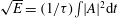 $\sqrt{E}=(1/{\it\tau})\!\int \!|A|^{2}\text{d}t$
, where
$\sqrt{E}=(1/{\it\tau})\!\int \!|A|^{2}\text{d}t$
, where
 $A$
is the wave envelope of the concurrent segment and
$A$
is the wave envelope of the concurrent segment and
 ${\it\tau}$
is the time window, to eliminate the initial current-induced increase of wave amplitude. An average and a standard deviation of the normalised maximum amplitude were calculated over the entire time series. The maximum normalised amplitude is presented as a function of
${\it\tau}$
is the time window, to eliminate the initial current-induced increase of wave amplitude. An average and a standard deviation of the normalised maximum amplitude were calculated over the entire time series. The maximum normalised amplitude is presented as a function of
 $U/c_{g}$
in figure 6 and compared with (4.2) and (4.3). Error bands equivalent to the 95 % confidence interval (two times the standard deviation) are also shown. Due to the stable current field in the wave flume, uncertainties are less noticeable than in the basins. Near the blocking limit (
$U/c_{g}$
in figure 6 and compared with (4.2) and (4.3). Error bands equivalent to the 95 % confidence interval (two times the standard deviation) are also shown. Due to the stable current field in the wave flume, uncertainties are less noticeable than in the basins. Near the blocking limit (
 $U/c_{g}\approx -0.4$
), where waves break and the current is less stable, confidence intervals are more substantial. The non-uniformity of the current field in the basins, on the other hand, resulted in a large uncertainty throughout the range of current speeds.
$U/c_{g}\approx -0.4$
), where waves break and the current is less stable, confidence intervals are more substantial. The non-uniformity of the current field in the basins, on the other hand, resulted in a large uncertainty throughout the range of current speeds.


Qualitatively, the tests are consistent with theory, substantiating the destabilising effect of the current. Quantitatively, (4.3) represents well the records for mild currents (
 $-0.1\leqslant U/c_{g}\leqslant 0$
), while (4.2) better predicts the maximum amplification for stronger currents (
$-0.1\leqslant U/c_{g}\leqslant 0$
), while (4.2) better predicts the maximum amplification for stronger currents (
 $-0.5<U/c_{g}\leqslant -0.1$
). Notable deviation from (4.2) occurs at the onset of blocking (
$-0.5<U/c_{g}\leqslant -0.1$
). Notable deviation from (4.2) occurs at the onset of blocking (
 $U/c_{g}\approx -0.5$
) in the wave flume due to breaking dissipation, as this is not accounted for in the model (no breaking was observed for
$U/c_{g}\approx -0.5$
) in the wave flume due to breaking dissipation, as this is not accounted for in the model (no breaking was observed for
 $U/c_{g}\geqslant -0.4$
in the flume). Current non-uniformity in the basins, on the other hand, increased the breaking probability well below the blocking speed. For the more regular current at Plymouth University, departure from (4.2) occurs for
$U/c_{g}\geqslant -0.4$
in the flume). Current non-uniformity in the basins, on the other hand, increased the breaking probability well below the blocking speed. For the more regular current at Plymouth University, departure from (4.2) occurs for
 $U/c_{g}\leqslant -0.3$
. A more pronounced non-uniformity and breaking probability at the University of Tokyo result in levelling off of the amplitude already at
$U/c_{g}\leqslant -0.3$
. A more pronounced non-uniformity and breaking probability at the University of Tokyo result in levelling off of the amplitude already at
 $U/c_{g}\approx -0.2$
. Nevertheless, (4.2) still represents the upper limit of the observations for
$U/c_{g}\approx -0.2$
. Nevertheless, (4.2) still represents the upper limit of the observations for
 $-0.3<U/c_{g}\leqslant -0.2$
. The deviation is statistically significant for stronger currents.
$-0.3<U/c_{g}\leqslant -0.2$
. The deviation is statistically significant for stronger currents.
5. Evolution of random wavefields
5.1. Significant wave height and wave spectrum
The evolution of significant wave height as a function of the dimensionless distance from the wavemaker is presented in figures 7 and 8 for experiments in the basins at Plymouth University and the University of Tokyo respectively. In the absence of a current,
 $H_{s}$
remains stable along the tank. Modulational instability has only a marginal effect and it results in a weak spectral downshift (see examples of spectral evolution in figure 9) (cf. Yuen & Lake Reference Yuen and Lake1982; Dias & Kharif Reference Dias and Kharif1999; Dysthe et al.
Reference Dysthe, Trulsen, Krogstad and Socquet-Juglard2003). For directional wavefields (figure 9
b), the downshift is slightly more accentuated due to a higher initial wave steepness. Wave breaking was not detected.
$H_{s}$
remains stable along the tank. Modulational instability has only a marginal effect and it results in a weak spectral downshift (see examples of spectral evolution in figure 9) (cf. Yuen & Lake Reference Yuen and Lake1982; Dias & Kharif Reference Dias and Kharif1999; Dysthe et al.
Reference Dysthe, Trulsen, Krogstad and Socquet-Juglard2003). For directional wavefields (figure 9
b), the downshift is slightly more accentuated due to a higher initial wave steepness. Wave breaking was not detected.

Figure 7. Evolution of the significant wave height
 $H_{s}$
as a function of the normalised distance from the wavemaker in the wave basin at Plymouth University: unidirectional wavefields (◼); directional wavefields (⚫).
$H_{s}$
as a function of the normalised distance from the wavemaker in the wave basin at Plymouth University: unidirectional wavefields (◼); directional wavefields (⚫).

Figure 8. Evolution of the significant wave height
 $H_{s}$
as a function of the normalised distance from the wavemaker in the wave basin at the University of Tokyo: unidirectional wavefields (◼); directional wavefields (⚫).
$H_{s}$
as a function of the normalised distance from the wavemaker in the wave basin at the University of Tokyo: unidirectional wavefields (◼); directional wavefields (⚫).

Figure 9. Example of spectral evolution with and without current for unidirectional (a) and directional (b) wavefields. The data are from tests in the wave basin at Plymouth University (similar spectra were detected at the University of Tokyo).
The interaction between waves and an opposing current generates an immediate increase of significant wave height (figures 7 and 8). Variability of the current field (in both space and time) further enhances
 $H_{s}$
along the tank. The adverse current gradient also induces a compression of the wavelength, forcing the dominant wavenumber to increase. This occurs within the first metre of propagation, where the gradient is at its maximum. This wave transformation implies an increase of the steepness (as an example,
$H_{s}$
along the tank. The adverse current gradient also induces a compression of the wavelength, forcing the dominant wavenumber to increase. This occurs within the first metre of propagation, where the gradient is at its maximum. This wave transformation implies an increase of the steepness (as an example,
 $k_{p}H_{s}/2$
grows up to approximately 0.1 for
$k_{p}H_{s}/2$
grows up to approximately 0.1 for
 $U/c_{g}\approx -0.15$
, while
$U/c_{g}\approx -0.15$
, while
 $k_{p}H_{s}/2\approx 0.16$
for
$k_{p}H_{s}/2\approx 0.16$
for
 $U/c_{g}\approx -0.30$
) and results in an amplification of nonlinearity (modulation instability). As a consequence, a more substantial (and quicker) downshift of the spectral peak takes place along the basins. This is already clear from records at the first probe (approximately three wavelengths from the wavemaker).
$U/c_{g}\approx -0.30$
) and results in an amplification of nonlinearity (modulation instability). As a consequence, a more substantial (and quicker) downshift of the spectral peak takes place along the basins. This is already clear from records at the first probe (approximately three wavelengths from the wavemaker).
While no notable dissipation was detected during the tests at Plymouth University, the significant wave height dropped after approximately 20 wavelengths for
 $U/c_{g}<-0.19$
at the University of Tokyo (see the squares in figure 8). This was recorded for both unidirectional and directional wavefields as a result of current-induced breaking.
$U/c_{g}<-0.19$
at the University of Tokyo (see the squares in figure 8). This was recorded for both unidirectional and directional wavefields as a result of current-induced breaking.
5.2. Occurrence of extremes: unidirectional wavefields
The occurrence of extreme waves is normally highlighted by the fourth-order moment of the probability density function of the surface elevation, i.e. the kurtosis (see, for example, Onorato et al. Reference Onorato, Cavaleri, Fouques, Gramstad, Janssen, Monbaliu, Osborne, Pakozdi, Serio, Stansberg, Toffoli and Trulsen2009a ). For Gaussian (linear) processes, the kurtosis is equal to 3 (e.g. Ochi Reference Ochi1998), while it increases slightly for weakly non-Gaussian waves (see, for example, Socquet-Juglard et al. Reference Socquet-Juglard, Dysthe, Trulsen, Krogstad and Liu2005; Onorato et al. Reference Onorato, Cavaleri, Fouques, Gramstad, Janssen, Monbaliu, Osborne, Pakozdi, Serio, Stansberg, Toffoli and Trulsen2009a ; Waseda et al. Reference Waseda, Kinoshita and Tamura2009).
The evolution of kurtosis in unidirectional wavefields as a function of distance from the wavemaker is shown in figures 10 and 11 (squares). Tests in the basins at Plymouth University and at the University of Tokyo respectively are presented. With no current, the initial conditions ensure a weak effect of modulational instability on the wave dynamics. Although the kurtosis grows slightly throughout the tanks, it only deviates weakly from Gaussian statistics (the kurtosis reaches a maximum of approximately 3.2). This deviation is primarily dominated by bound waves.

Figure 10. Evolution of kurtosis as a function of the normalised distance from the wavemaker in the wave basin at Plymouth University: unidirectional wavefields (◼); directional wavefields (⚫).

Figure 11. Evolution of kurtosis as a function of the normalised distance from the wavemaker in the wave basin at the University of Tokyo: unidirectional wavefields (◼); directional wavefields (⚫).
Amplification of wave nonlinearity due to current makes the growth of kurtosis more prominent. Deviations from Gaussian statistics become more substantial with increase of the current gradient, corroborating a transition from weakly to strongly non-Gaussian statistics. Significantly large values of the kurtosis (
 ${>}4$
) are reached after approximately 25 wavelengths for current speeds of
${>}4$
) are reached after approximately 25 wavelengths for current speeds of
 $U/c_{g}\approx -0.15$
and
$U/c_{g}\approx -0.15$
and
 $-0.24$
at Plymouth University and
$-0.24$
at Plymouth University and
 $U/c_{g}\approx -0.13$
and
$U/c_{g}\approx -0.13$
and
 $-0.19$
at the University of Tokyo. In this regard, the evolution of kurtosis is qualitatively consistent with the dynamical behaviour recorded for more nonlinear systems in the absence of current (see, for example, Onorato et al.
Reference Onorato, Cavaleri, Fouques, Gramstad, Janssen, Monbaliu, Osborne, Pakozdi, Serio, Stansberg, Toffoli and Trulsen2009a
,Reference Onorato, Waseda, Toffoli, Cavaleri, Gramstad, Janssen, Kinoshita, Monbaliu, Mori, Osborne, Serio, Stansberg, Tamura and Trulsen
b
; Waseda et al.
Reference Waseda, Kinoshita and Tamura2009). It should be noted that the percentage of breakers in the records (i.e. waves with steepness
$-0.19$
at the University of Tokyo. In this regard, the evolution of kurtosis is qualitatively consistent with the dynamical behaviour recorded for more nonlinear systems in the absence of current (see, for example, Onorato et al.
Reference Onorato, Cavaleri, Fouques, Gramstad, Janssen, Monbaliu, Osborne, Pakozdi, Serio, Stansberg, Toffoli and Trulsen2009a
,Reference Onorato, Waseda, Toffoli, Cavaleri, Gramstad, Janssen, Kinoshita, Monbaliu, Mori, Osborne, Serio, Stansberg, Tamura and Trulsen
b
; Waseda et al.
Reference Waseda, Kinoshita and Tamura2009). It should be noted that the percentage of breakers in the records (i.e. waves with steepness
 $kH/2$
exceeding the threshold for the onset of breaking, Babanin et al.
Reference Babanin, Chalikov, Young and Savelyev2007) is below 10 %. For stronger currents, increase of breaking probability (breakers exceed 60 % of the total number of individual waves) limits the growth of kurtosis. This is particularly clear from the experiments at the University of Tokyo, where the kurtosis remains basically constant (and relatively close to the Gaussian value of 3) for
$kH/2$
exceeding the threshold for the onset of breaking, Babanin et al.
Reference Babanin, Chalikov, Young and Savelyev2007) is below 10 %. For stronger currents, increase of breaking probability (breakers exceed 60 % of the total number of individual waves) limits the growth of kurtosis. This is particularly clear from the experiments at the University of Tokyo, where the kurtosis remains basically constant (and relatively close to the Gaussian value of 3) for
 $U/c_{g}\Leftarrow -0.26$
.
$U/c_{g}\Leftarrow -0.26$
.

Figure 12. Kurtosis as a function of
 $U/C_{g}$
for unidirectional (a) and directional (b) wavefields: experimental data from the directional wave basin at Plymouth University (◼) and experimental data from the directional wave basin at the University of Tokyo (▲).
$U/C_{g}$
for unidirectional (a) and directional (b) wavefields: experimental data from the directional wave basin at Plymouth University (◼) and experimental data from the directional wave basin at the University of Tokyo (▲).
Despite slight differences in the actual steepness, records in both basins show a similar quantitative dependence of the maximum kurtosis upon the normalised current velocity
 $U/c_{g}$
(see figure 12
a). It is worth mentioning that the maximum enhancement of kurtosis is approximately 35 %. Higher breaking probability (
$U/c_{g}$
(see figure 12
a). It is worth mentioning that the maximum enhancement of kurtosis is approximately 35 %. Higher breaking probability (
 ${>}60\,\%$
) due to a more non-uniform current at the University of Tokyo produces a clear decay of kurtosis already for
${>}60\,\%$
) due to a more non-uniform current at the University of Tokyo produces a clear decay of kurtosis already for
 $U/c_{g}\Leftarrow -0.2$
(i.e. well before the blocking limit).
$U/c_{g}\Leftarrow -0.2$
(i.e. well before the blocking limit).
It is also instructive to present the deviation from Gaussian statistics in terms of exceedance probability of wave height,
 $P(H)$
. In figure 13(a,b), the wave height distribution at maximum kurtosis is shown for
$P(H)$
. In figure 13(a,b), the wave height distribution at maximum kurtosis is shown for
 $U/c_{g}\approx -0.1$
. The wave height distribution in the absence of current and the Rayleigh distribution are included for reference. The wave height is non-dimensionalised by means of four times the standard deviation (namely, the significant wave height of the related time series). In the absence of adverse currents, the exceedance probability for the wave height fits, as expected, the Rayleigh distribution (cf. Ochi Reference Ochi1998), although larger waves in the basin at the University of Tokyo are slightly underpredicted. The presence of current, on the other hand, induces a substantial deviation from the Rayleigh distribution, which clearly underpredicts the occurrence of waves with
$U/c_{g}\approx -0.1$
. The wave height distribution in the absence of current and the Rayleigh distribution are included for reference. The wave height is non-dimensionalised by means of four times the standard deviation (namely, the significant wave height of the related time series). In the absence of adverse currents, the exceedance probability for the wave height fits, as expected, the Rayleigh distribution (cf. Ochi Reference Ochi1998), although larger waves in the basin at the University of Tokyo are slightly underpredicted. The presence of current, on the other hand, induces a substantial deviation from the Rayleigh distribution, which clearly underpredicts the occurrence of waves with
 $H/4{\it\sigma}>1.5$
. It is interesting to note, in this regard, that the probability of occurrence of extreme and rogue waves (
$H/4{\it\sigma}>1.5$
. It is interesting to note, in this regard, that the probability of occurrence of extreme and rogue waves (
 $H/4{\it\sigma}>2$
) increases by more than one order of magnitude (from a probability level of
$H/4{\it\sigma}>2$
) increases by more than one order of magnitude (from a probability level of
 $3.5\times 10^{-4}$
to
$3.5\times 10^{-4}$
to
 $6.5\times 10^{-3}$
). This is consistent with strong deviations from the Rayleigh distribution, which were observed numerically and experimentally in unidirectional wavefields with Benjamin–Feir index approximately equal to 1 (Socquet-Juglard et al.
Reference Socquet-Juglard, Dysthe, Trulsen, Krogstad and Liu2005; Onorato et al.
Reference Onorato, Osborne, Serio, Cavaleri, Brandini and Stansberg2006).
$6.5\times 10^{-3}$
). This is consistent with strong deviations from the Rayleigh distribution, which were observed numerically and experimentally in unidirectional wavefields with Benjamin–Feir index approximately equal to 1 (Socquet-Juglard et al.
Reference Socquet-Juglard, Dysthe, Trulsen, Krogstad and Liu2005; Onorato et al.
Reference Onorato, Osborne, Serio, Cavaleri, Brandini and Stansberg2006).

Figure 13. Wave height distribution: unidirectional wavefields (a,b); directional wavefields (c,d).
An independent verification of such a remarkable result was achieved in the wave flume at Plymouth University. Records confirmed a clear transition from weakly to strongly non-Gaussian properties with increase of
 $U/c_{g}$
(see the dependence of kurtosis on current speed in figure 14). Qualitatively, this trend is consistent with the one recorded in the basins, with a maximum occurring at
$U/c_{g}$
(see the dependence of kurtosis on current speed in figure 14). Qualitatively, this trend is consistent with the one recorded in the basins, with a maximum occurring at
 $U/c_{g}\approx -0.3$
. The maximum enhancement of kurtosis is approximately 15 %. In the proximity of the blocking limit
$U/c_{g}\approx -0.3$
. The maximum enhancement of kurtosis is approximately 15 %. In the proximity of the blocking limit
 $U/c_{g}\leqslant -0.4$
, the trend levels off due to breaking dissipation.
$U/c_{g}\leqslant -0.4$
, the trend levels off due to breaking dissipation.

Figure 14. Kurtosis as a function of
 $U/C_{g}$
in the wave flume at Plymouth University (unidirectional wavefield).
$U/C_{g}$
in the wave flume at Plymouth University (unidirectional wavefield).
5.3. Occurrence of extremes: directional wavefields
In realistic oceanic conditions, wave energy spreads over a range of directions. This normally results in a stabilisation of wavepackets, which suppresses any development of strong non-Gaussian properties. The effect of wave–current interaction on the kurtosis for fairly narrow directional sea states (
 $N=50$
, i.e. a narrow swell) is here discussed (see the circles in figures 10 and 11).
$N=50$
, i.e. a narrow swell) is here discussed (see the circles in figures 10 and 11).
The kurtosis remains steady throughout the basin and deviates only weakly from Gaussianity without current, despite a rather strong initial steepness. Similarly to the unidirectional wavefield, such a deviation is linked to the bound-wave contribution (cf. Socquet-Juglard et al.
Reference Socquet-Juglard, Dysthe, Trulsen, Krogstad and Liu2005; Onorato et al.
Reference Onorato, Cavaleri, Fouques, Gramstad, Janssen, Monbaliu, Osborne, Pakozdi, Serio, Stansberg, Toffoli and Trulsen2009a
; Waseda et al.
Reference Waseda, Kinoshita and Tamura2009). By applying a gradually stronger adverse current, however, the kurtosis shows a clear dynamical behaviour. While the kurtosis remains lower than its values for unidirectional waves, a transition from weakly to non-Gaussian statistics can be recognised. This is especially evident under the influence of the more regular current field at Plymouth University. In both basins, nonetheless, this transition is achieved at
 $U/c_{g}\approx -0.25$
. A quantitative comparison of the maximum kurtosis as a function of
$U/c_{g}\approx -0.25$
. A quantitative comparison of the maximum kurtosis as a function of
 $U/c_{g}$
is reported in figure 12(b). It is interesting to note that there is a substantial difference in terms of maximum kurtosis in the two basins. Although the qualitative behaviour is similar, the kurtosis at Plymouth University reaches a much higher value than at the University of Tokyo (
$U/c_{g}$
is reported in figure 12(b). It is interesting to note that there is a substantial difference in terms of maximum kurtosis in the two basins. Although the qualitative behaviour is similar, the kurtosis at Plymouth University reaches a much higher value than at the University of Tokyo (
 ${\approx}3.5$
at Plymouth University and
${\approx}3.5$
at Plymouth University and
 ${\approx}3.3$
at the University of Tokyo). Again, this is primarily due to a higher breaking probability at the University of Tokyo as a result of current non-uniformity.
${\approx}3.3$
at the University of Tokyo). Again, this is primarily due to a higher breaking probability at the University of Tokyo as a result of current non-uniformity.
For completeness, the wave height distribution as recorded with and without the opposing current is presented in figure 13(c,d). As the initial wavefield can no longer be considered to be narrow banded, the wave height distribution is overestimated by the Rayleigh distribution in the absence of current (e.g. Ochi Reference Ochi1998). In the presence of an opposing current, large waves occur more often, lifting the tail of the distribution. A notable deviation from the Rayleigh distribution is clearly observed for the records at Plymouth University (the data at the University of Tokyo fit to a certain extent the Rayleigh distribution). It is worth mentioning that the current-induced enhancement of probability for a wave height larger than twice the significant wave height is nearly one order of magnitude.
6. Conclusions
The influence of an opposing current on the nonlinear dynamics of random waves and the probability of occurrence of extreme waves was assessed experimentally. Laboratory tests were carried out in three independent facilities: two wave basins (one at Plymouth University and one at the University of Tokyo), where propagation in two horizontal dimensions is allowed, and one wave flume at Plymouth University, which only allows propagation in one horizontal dimension. The evolution of wavefields was monitored by capacitance gauges distributed along the facilities. The current velocity was measured by means of electromagnetic current meters, propellers and ADVs.
In all facilities, it was first verified that the interaction with an opposing current leads to an amplification of the modulation of marginally unstable regular wavepackets. The extent of the amplification was found to depend on a dimensionless current velocity (
 $U/c_{g}$
). It is worth noting that directional wave focusing due to current-induced refraction, as a result of cross-tank flow variations, and sidewall reflection limited wave amplification in the basin at the University of Tokyo.
$U/c_{g}$
). It is worth noting that directional wave focusing due to current-induced refraction, as a result of cross-tank flow variations, and sidewall reflection limited wave amplification in the basin at the University of Tokyo.
Tests were then conducted with irregular waves to trace the effect of the opposing current on the occurrence of extremes. Unidirectional and directional random sea states were investigated. The initial conditions at the wavemaker were given in the form of an input JONSWAP-like wave spectrum to model waves in the frequency domain and a
 $\cos ^{N}({\it\vartheta})$
function to describe the directional spreading. For tests in the wave basins, the wave steepness
$\cos ^{N}({\it\vartheta})$
function to describe the directional spreading. For tests in the wave basins, the wave steepness
 $k_{p}H_{s}/2$
(a measure of the degree of nonlinearity of the system) was set equal to 0.062 at Plymouth University and equal to 0.063 at the University of Tokyo for unidirectional wavefields. Tests in the wave flume were undertaken with different sea states with smaller steepness (
$k_{p}H_{s}/2$
(a measure of the degree of nonlinearity of the system) was set equal to 0.062 at Plymouth University and equal to 0.063 at the University of Tokyo for unidirectional wavefields. Tests in the wave flume were undertaken with different sea states with smaller steepness (
 $k_{p}H_{s}/2=0.05$
) to independently confirm the findings. When current is not applied, the selected wave steepness is sufficiently low to keep wave statistics weakly non-Gaussian (i.e. nonlinear effects are dominated by bound waves). For directional wavefields,
$k_{p}H_{s}/2=0.05$
) to independently confirm the findings. When current is not applied, the selected wave steepness is sufficiently low to keep wave statistics weakly non-Gaussian (i.e. nonlinear effects are dominated by bound waves). For directional wavefields,
 $k_{p}H_{s}/2=0.12$
. A directional spreading of
$k_{p}H_{s}/2=0.12$
. A directional spreading of
 $N=50$
was applied, which represents a fairly narrow swell. Despite the high steepness (the values represent storm conditions), the directional spreading suppresses nonlinear dynamics, keeping the wave statistics weakly non-Gaussian in the absence of the current.
$N=50$
was applied, which represents a fairly narrow swell. Despite the high steepness (the values represent storm conditions), the directional spreading suppresses nonlinear dynamics, keeping the wave statistics weakly non-Gaussian in the absence of the current.
Benchmark tests were first undertaken in the absence of the background current. Experiments were then repeated with an opposing current with velocity ranging from a small fraction to half the group velocity. It should be noted that the current outlets were located on the floors of the basins in the proximity of the wavemaker. This particular configuration ensured that the current speed was approximately zero near the wavemaker so that waves were actually generated in a condition of no current. Regime speeds were observed a few metres from the wavemaker. In order to gather enough data for stable statistics, two 1 h long realisations were carried out with different random amplitudes and random phases. The analysis was mainly concentrated on the fourth-order moment of the probability density function of the surface elevation, namely the kurtosis, which is a measure of the probability of extremes in the record.
Generally speaking, the interaction with an opposing current forces the wave profile to compress. Therefore, while the wavelength shortens, the significant wave height increases as a function of current speed. Due to temporal and spatial variability of the current, a slight increase of significant wave height also occurred along the facilities. More substantial non-uniformity at the University of Tokyo, nonetheless, led to breaking dissipation, especially for strong currents. The transformation of wave profile increases the steepness and hence strengthens the nonlinearity. In the first instance, this accelerates nonlinear energy transfer, making the spectral downshifting more prominent. Further, it amplifies effects related to modulational instability, increasing the occurrence of extremes. This is corroborated by a gradual transition from weakly to strongly non-Gaussian properties along the basins. For a current speed of
 $U/c_{g}\approx -0.25$
, the kurtosis reached its maximum (a value above 4), approximately 30 % higher than the value expected without current. For such a kurtosis, wave heights greater than twice the significant wave height occurred with a probability of occurrence of approximately
$U/c_{g}\approx -0.25$
, the kurtosis reached its maximum (a value above 4), approximately 30 % higher than the value expected without current. For such a kurtosis, wave heights greater than twice the significant wave height occurred with a probability of occurrence of approximately
 $6.5\times 10^{-3}$
, which is an order of magnitude greater than the probability level specified by the Rayleigh distribution. With stronger and more non-uniform currents, the number of extremes dropped notably due to wave breaking, suppressing the development of strong non-Gaussian statistics. Qualitatively, this result is confirmed by the independent tests in the wave flume. Despite a lower degree of nonlinearity (lower steepness), records from the wave flume also show a robust increase of kurtosis as a function of
$6.5\times 10^{-3}$
, which is an order of magnitude greater than the probability level specified by the Rayleigh distribution. With stronger and more non-uniform currents, the number of extremes dropped notably due to wave breaking, suppressing the development of strong non-Gaussian statistics. Qualitatively, this result is confirmed by the independent tests in the wave flume. Despite a lower degree of nonlinearity (lower steepness), records from the wave flume also show a robust increase of kurtosis as a function of
 $U/c_{g}$
.
$U/c_{g}$
.
Qualitatively, a similar result was also replicated for more realistic directional sea states. Although directionality suppresses the effect of modulational instability on wave statistics (namely, the increase of kurtosis), the interaction with an opposing current seems to be capable of compensating the influence of directional spreading. As a result, the kurtosis gradually increases with increase of the current speed (
 $U/c_{g}$
), reaching a maximum increment (with respect to the case with no current) of approximately 15 %.
$U/c_{g}$
), reaching a maximum increment (with respect to the case with no current) of approximately 15 %.
Despite some quantitative differences, mainly due to current variability, our results have indicated in a robust and consistent manner that the presence of a current is capable of amplifying nonlinear wave dynamics and thus can enhance the occurrence of extremes in a random wavefield. The extent of this amplification depends on the ratio of current speed to group velocity (
 $U/c_{g}$
) and current non-uniformity, which induces breaking dissipation well before the blocking limit.
$U/c_{g}$
) and current non-uniformity, which induces breaking dissipation well before the blocking limit.
Acknowledgements
The experiments were supported by the JSPS Fellowship for Research in Japan Program, Grants-in-Aid for Scientific Research of the JSPS and the International Science Linkages (ISL) Program of the Australian Academy of Science. L.C. has contributed under the EU-funded MyWave FP7-SPACE-2011-1/CP-FP project. A.T. and D.G. acknowledge Dr K. Collins and Dr M. Hann for providing velocity measurements in the wave flume and ocean wave basin at Plymouth University. T.W. was supported by JSPS KAKENHI Grant-in-Aid for Scientific Research and Grant-in-Aid for Young Scientists. M.O. and A.T. acknowledge the VDRS grant from Swinburne University of Technology. M.O. was supported by MIUR Grant PRIN 2012BFNWZ2 and ONR grant N000141010991. M.O. also acknowledges Dr B. GiuliNico for interesting discussions.


