


1. Introduction
Richtmyer–Meshkov (RM) instability is initiated when a shock wave interacts with an interface between two fluids of different densities (Richtmyer Reference Richtmyer1960; Meshkov Reference Meshkov1969), and further induces mushroom-shaped flow structures such as bubbles (light fluids penetrating into heavy ones) and spikes (heavy fluids penetrating into light ones), which finally may cause a flow transition to turbulent mixing (Zhou, Robey & Buckingham Reference Zhou, Robey and Buckingham2003; Zhou Reference Zhou2007; Zhou et al. Reference Zhou, Clark, Clark, Glendinning, Skinner, Huntington, Hurricane, Dimits and Remington2019). Over the past few decades, the RM instability has become a subject of intensive research due to its crucial role in various industrial and scientific fields such as inertial confinement fusion (ICF) (Lindl et al. Reference Lindl, Landen, Edwards, Moses and Team2014) and supernova explosion (Kuranz et al. Reference Kuranz2018). For example, the RM instability determines the seeds of Rayleigh–Taylor (RT) instability (Rayleigh Reference Rayleigh1883; Taylor Reference Taylor1950) that develops during the implosion in ICF (Goncharov Reference Goncharov1999). The mixing of hot fuel inside with cooler shell material outside, induced by RM and RT instabilities in the target of ICF, significantly reduces and even eliminates the thermonuclear yield (Miles et al. Reference Miles, Edwards, Blue, Hansen, Robey, Drake, Kuranz and Leibrandt2004). The RM instability on a single-mode interface has been extensively studied due to its fundamental significance (Brouillette Reference Brouillette2002; Zhou Reference Zhou2017a,Reference Zhoub; Zhai et al. Reference Zhai, Zou, Wu and Luo2018). However, the initial perturbation in reality is essentially multi-mode with wavenumbers spanning many orders of magnitude, and whether the perturbation growth of a multi-mode RM instability depends on the initial spectrum or not is crucial to ICF (Miles et al. Reference Miles, Edwards, Blue, Hansen, Robey, Drake, Kuranz and Leibrandt2004) but remains unclear.
Theoretically, there are mainly six kinds of models describing the perturbation growth of a multi-mode interface: the linear model, the modal model, the potential model, the vortex model, the perturbation expansion model and the group theory approach. Based on the principle that each individual mode develops independently in linear stages, Mikaelian (Reference Mikaelian2005) proposed the linear model to describe the multi-mode interface evolution by summing the time-varying amplitude growth of each mode. Haan (Reference Haan1989) found that the constituent modes with similar wavelengths of a multi-mode interface add up to create an effective local large amplitude, and, therefore, the onset of the nonlinear stage of a multi-mode perturbation is earlier than that of the classical single-mode case. Subsequently, Haan (Reference Haan1991) proposed the modal model with second-order accuracy to quantify the mode-competition effect on the perturbation growth of each mode in the early nonlinear stage. The modal model and its extended types have achieved a wide range of validation in RT instability issues (Remington et al. Reference Remington, Weber, Marinak, Haan, Kilkenny, Wallace and Dimonte1995; Ofer et al. Reference Ofer, Alon, Shvarts, McCrory and Verdon1996; Elbaz & Shvarts Reference Elbaz and Shvarts2018), but their application to the RM instability is still lacking. Assuming that mode competition is absent before a bubble reaches its asymptotic growth, the potential model was proposed by Alon et al. (Reference Alon, Hecht, Mukamel and Shvarts1994) and Layzer (Reference Layzer1955) to predict the eventual average bubble distribution and the growth rate. However, the potential model is invalid when the Atwood number (defined as  $A=(\rho _2-\rho _1)/(\rho _2+\rho _1)$, with
  $\rho _1$ and
  $\rho _2$ being the densities of light fluid and heavy fluid, respectively) is low. When the Atwood number approaches zero, the vortex model (Jacobs & Sheeley Reference Jacobs and Sheeley1996) was adopted by Rikanati, Alon & Shvarts (Reference Rikanati, Alon and Shvarts1998) to make up the bubble asymptotic growth rate. Note that both the potential model (Alon et al. Reference Alon, Hecht, Mukamel and Shvarts1994, Reference Alon, Hecht, Ofer and Shvarts1995; Oron et al. Reference Oron, Arazi, Kartoon, Rikanati, Alon and Shvarts2001) and the vortex model (Rikanati et al. Reference Rikanati, Alon and Shvarts1998) involve a self-similar growth of the bubble front which is independent of the initial spectrum, and both models obtain a 1/
 $t$ decay for the late-time bubble growth rate in a multi-mode RM instability. The perturbation expansion model developed by Zhang & Sohn (Reference Zhang and Sohn1997) was extended by Vandenboomgaerde, Gauthier & Mügler (Reference Vandenboomgaerde, Gauthier and Mügler2002) to predict the early nonlinear amplitude growth of the constituent modes of a multi-mode interface by retaining only the terms with the highest power in time. The group theory approach (Abarzhi Reference Abarzhi2008, Reference Abarzhi2010; Pandian, Stellingwerf & Abarzhi Reference Pandian, Stellingwerf and Abarzhi2017) identifies the connection between the symmetry properties of the interface morphology and the relative phases of waves constituting the interface perturbation.
Experimentally, shock-tube experiments were performed to investigate two-bubble competition (Sadot et al. Reference Sadot, Erez, Alon, Oron, Levin, Erez, Ben-Dor and Shvarts1998), and the results showed that the growth of the larger (or smaller) bubble is promoted (or suppressed). Dimonte & Schneider (Reference Dimonte and Schneider2000) conducted a series of three-dimensional linear electric motor experiments to investigate multi-mode RT and RM instabilities, and found that the density ratio has a limited effect on the self-similar growth factor for the bubble. When the density ratio is large, the self-similar growth factor for the spike is clearly larger than that for the bubble counterpart. The multi-mode RM instability of two liquids was investigated by Niederhaus & Jacobs (Reference Niederhaus and Jacobs2003), and the development of the multi-mode perturbation was found to be strongly dependent on the relative amplitudes of initial modes. The growth of the multi-mode interface perturbation created by the gas curtain technique shows a weak dependence on the initial conditions (Balasubramanian, Orlicz & Prestridge Reference Balasubramanian, Orlicz and Prestridge2013). Experiments of a dual-mode interface RM instability under high-Mach-number conditions have been performed (Di Stefano et al. Reference Di Stefano, Malamud, Kuranz, Klein and Drake2015a,Reference Di Stefano, Malamud, Kuranz, Klein, Stoeckl and Drakeb), and the results indicated that new modes are generated from the mode-competition effect, and the perturbations of these modes grow and saturate over time. The dual-mode RM instability under weak shock conditions was also considered, from which the mode-competition effect on the RM instability development cannot be ignored when the wavenumber of one constituent mode is twice that of the other constituent mode (Luo et al. Reference Luo, Liu, Liang, Ding and Wen2020). The mixing of a multi-mode interface was investigated by Mohaghar et al. (Reference Mohaghar, Carter, Musci, Reilly, McFarland and Ranjan2017) using density and velocity statistics, and the flow shows a distinct memory of initial conditions, the long-wavelength perturbation having a strong influence on the interface development. Recently, developments of quasi-single-mode interfaces created by the soap film technique in the early nonlinear stage have been studied, and the effect of high-order modes on the perturbation growth was highlighted to distinguish from single-mode perturbation (Liang et al. Reference Liang, Zhai, Ding and Luo2019). A near-sinusoidal interface dominated by one mode was generated by a novel membraneless technique where cross-flowing air was separated from SF $_6$ by an oscillating splitter plate (Mansoor et al. Reference Mansoor, Dalton, Martinez, Desjardins, Charonko and Prestridge2020), and the effects of the initial amplitude on the perturbation width growth and mixing transition have been discussed, and earlier mixing transitions for higher amplitude-to-wavelength ratio cases are noted from experiments.
Numerically, it is commonly realized that the phases of the constituent modes influence multi-mode perturbation growth (Vandenboomgaerde et al. Reference Vandenboomgaerde, Gauthier and Mügler2002; Miles et al. Reference Miles, Edwards, Blue, Hansen, Robey, Drake, Kuranz and Leibrandt2004; Pandian et al. Reference Pandian, Stellingwerf and Abarzhi2017). Besides, the self-similar growth factor of the late-time RM instability has a dependence on the scale of the initial spectrum. Specifically, a broadband perturbation leads to a larger bubble growth factor than a narrowband counterpart (Thornber et al. Reference Thornber, Drikakis, Youngs and Williams2010; Liu & Xiao Reference Liu and Xiao2016; Thornber Reference Thornber2016; Groom & Thornber Reference Groom and Thornber2020).
Although significant progress on the multi-mode RM instability has been made, the quantitative relation between initial conditions and perturbation growth is still unclear mainly because a general nonlinear theory for predicting the multi-mode perturbation width growth is absent, and elaborate experiments on the multi-mode RM instability with controllable initial conditions are very limited. In our previous work, the extended soap-film technique was utilized to create a classical two-dimensional (2-D) single-mode perturbation (Liu et al. Reference Liu, Liang, Ding, Liu and Luo2018), a 2-D multi-mode interface dominated by only one mode (Liang et al. Reference Liang, Zhai, Ding and Luo2019) and a 2-D multi-mode interface dominated by two modes (Luo et al. Reference Luo, Liu, Liang, Ding and Wen2020). The initial perturbations of these interfaces were precisely designed and the initial conditions were well controlled. In this work, a 2-D complex multi-mode interface constituted of various modes is first formed, and shock-tube experiments on the developments of eight kinds of air–SF $_6$ multi-mode interface are performed. Then, new nonlinear theories based on the initial spectrum, shock intensity and density ratio are proposed to predict each mode amplitude growth and the total perturbation width growth of a 2-D multi-mode interface.
2. Experimental method
The extended soap-film technique, which has been widely used in our previous work (Ding et al. Reference Ding, Si, Chen, Zhai, Lu and Luo2017; Liu et al. Reference Liu, Liang, Ding, Liu and Luo2018; Liang et al. Reference Liang, Zhai, Ding and Luo2019), is adopted to generate a periodic multi-mode interface with a controllable initial shape to separate SF $_{6}$ from air. Such a technique can largely eliminate the short-wavelength perturbations, diffusion layer and three-dimensionality of the formed interface (Liu et al. Reference Liu, Liang, Ding, Liu and Luo2018; Liang et al. Reference Liang, Zhai, Ding and Luo2019). As shown in figure 1(a), two transparent devices with an inner height of 7.0 mm and a width of 140.0 mm are first made using acrylic plates (3.0 mm in thickness). A groove (0.7 mm in thickness and 0.5 mm in width) with a multi-mode shape is then manufactured on the internal side of each plate by a high-precision engraving machine. Then, two thin filaments (1.0 mm in thickness and 0.5 mm in width) with the same multi-mode shape are mounted into the grooves of the upper and lower plates, respectively, to produce desired constraints. Therefore, the bulging of the filament into the flow is less than 0.3 mm, and has a negligible effect on the flow field. A small rectangular frame wetted by soap solution (78 % distilled water, 2 % sodium oleate and 20 % glycerine by mass) is pulled along the filaments, and a quasi-2-D soap-film interface is immediately generated, as shown in figure 1(a). Subsequently, the auxiliary framework is gently inserted until it is completely connected to the corresponding device. After that, the framework with a soap film on its surface is slowly inserted into the test section of the shock tube. To form an air–SF
 $_6$ interface, the air on the right-hand side of the interface is replaced by SF
 $_6$. To minimize the effect of the shock-tube walls on interface evolution, a short flat part with 10 mm on each side of the perturbed interface is adopted, as sketched in figure 1(b), and its effect on the interface evolution is limited (Luo et al. Reference Luo, Liang, Si and Zhai2019).

Figure 1. Schematics of soap-film interface generation (a) and the initial configuration (b).
In the Cartesian coordinate system, as sketched in figure 1(b), the multi-mode interface investigated can be described as a sum of three cosine modes:
 \begin{equation} y=\sum_{1}^{3}a_{k_n}^{0}\cos(k_nx+\phi_{k_n}),\quad x\in[{-}60,60]\,\mathrm{mm}, \end{equation}
where  $a_{k_n}^{0}$,
  $k_n$ and
  $\phi _{k_n}$ respectively denote the initial amplitude, wavenumber and phase of the
  $n$th constituent mode with
  $n= 1$, 2 and 3. To illustrate the influences of the initial amplitude, wavenumber and relative phase on the 2-D multi-mode RM instability, eight different kinds of multi-mode interface are designed in this work. The initial spectrum and the initial perturbation width (
 $w_0$, sketched in figure 1b) of the multi-mode interface in different cases are listed in table 1. In this work,
  $\phi _{k1}$ is kept as 0 and
  $\phi _{k2}$ and
  $\phi _{k3}$ are varied. For convenience, the following notation is adopted:
  $\phi _{k2} = \phi _{k3} = 0$ (in-phase (IP) case);
  $\phi _{k2} = \phi _{k3} = {\rm \pi}$ (anti-phase (AP) case);
  $\phi _{k2} = 0$,
  $\phi _{k3} = {\rm \pi}$ (k
 $_3$AP case);
  $\phi _{k2} = {\rm \pi}$,
  $\phi _{k3} = 0$ (k
 $_2$AP case). The influence of the initial amplitude of mode
  $k_n$ on the RM instability can be studied by varying
  $a_{k_n}^{0}k_n$ (Mansoor et al. Reference Mansoor, Dalton, Martinez, Desjardins, Charonko and Prestridge2020; Sewell et al. Reference Sewell, Ferguson, Krivets and Jacobs2021). In this work, the cases of IP-s, k
 $_3$AP-s, k
 $_2$AP-s and AP-s are classified as small-
 $w_0$ cases, whereas the cases of IP-h, k
 $_3$AP-h, k
 $_2$AP-h and AP-h are classified as large-
 $w_0$ cases.
Table 1. Initial spectrum and initial perturbation width of multi-mode interfaces formed in the present work. Here  $a_{k_n}^{0}$,
  $k_n$ and
  $\phi _{k_n}$ denote the initial amplitude, wavenumber and phase of the
  $n$th constituent mode, respectively;
  $w_0$,
  $w_{0b}$ and
  $w_{0s}$ denote the initial total perturbation width, bubble width and spike width of the multi-mode interface, respectively. The unit for the amplitude and width is mm and for the wavenumber is m
 $^{-1}$.

The experiments are performed in a horizontal shock tube with a  $140\,\textrm {mm} \times 13$ mm cross-sectional area. This type of tube has been widely used in shock–interface interaction studies (Luo, Wang & Si Reference Luo, Wang and Si2013; Zhai et al. Reference Zhai, Wang, Si and Luo2014; Luo et al. Reference Luo, Wang, Si and Zhai2015; Ding et al. Reference Ding, Si, Chen, Zhai, Lu and Luo2017). The ambient pressure and temperature are 101.3 kPa and
  $299.5\pm 1.0$ K, respectively. In experiments, the incident shock wave with velocity (
 $v_s$) of
  $409\pm 1\,\textrm {m}\,\mathrm {s}^{-1}$ (the incident shock Mach number (
 $M$) is 1.18) moves from air to SF
 $_6$. The ambient air is considered as pure and the test gas is a mixture of air and SF
 $_6$, the mass fraction of SF
 $_6$ being
  $0.97\pm 0.01$ calculated according to one-dimensional gas dynamics theory. Meanwhile, the transmitted shock velocity (
 $v_t$) and the speed jump of the interface (
 ${\rm \Delta} v$) can be calculated as
  $182\pm 1\,\textrm {m}\,\mathrm {s}^{-1}$ and
  $65.5\pm 0.5\,\textrm {m}\,\textrm {s}^{-1}$, respectively. The post-shock Atwood number
  $A^{+}$ (defined as
  $A^{+}=(\rho _2^{+}-\rho _1^{+})/(\rho _2^{+}+\rho _1^{+})$, with
  $\rho _2^{+}$ and
  $\rho _1^{+}$ being the densities of shocked test gas and air, respectively) is
  $0.66\pm 0.01$. The flow field is monitored using high-speed schlieren photography. The frame rate of the high-speed video camera (FASTCAM SA5, Photron Limited) is 62 500 f.p.s. with a shutter time of 1
  $\mathrm {\mu }$s. The spatial resolution of the schlieren images is 0.4 mm pixel
 $^{-1}$. The visualization window of the flow field is within the range
  $x\in [-50,50]\,\mathrm {mm}$, as shown with the grey zone in figure 1(b). For each case, at least three experimental runs are performed, and the experiments have a good repeatability. The relative differences of the data among diverse experimental runs are within 3 %.
The three-dimensional feature of the initial soap-film interface is discussed. Because the gases on both sides of the interface are at ambient pressure, the soap-film interface formed has a zero mean curvature, and the geometry can be characterized as minimum surface (Luo et al. Reference Luo, Wang and Si2013; Liang et al. Reference Liang, Liu, Zhai, Si and Luo2021). For instance, half of the perturbation width of the soap-film interface in case IP-h or k $_3$AP-h is 4 mm (see table 1), indicating that the total amplitude of the soap-film interface on the boundary slice (i.e.
  $z=\pm 3.5$ mm) is 4 mm. The maximum wavelength of the soap-film interface is 60 mm, and the interface height is 7 mm. Based on our previous work (Luo et al. Reference Luo, Wang and Si2013; Liang et al. Reference Liang, Liu, Zhai, Si and Luo2021), the amplitude of the soap film on the symmetry slice (i.e.
  $z=0$ mm) is 3.75 mm. Therefore, the amplitude ratio of the symmetry slice over the boundary slice is 93.75 %. The absolute difference between the amplitudes on the symmetry slice and the boundary slice is about 0.25 mm, and is smaller than the size of a schlieren image's pixel. As a result, it is believed that the interface height of 7 mm can reduce the three-dimensional effect in this work.
The boundary layer effect on the interface evolution is also considered. After the incident shock with  $M$ of 1.18 impacts the interface, the flow behind the transmitted shock can be regarded as laminar and incompressible. As a result, the displacement thickness of the boundary layer (
 $\delta ^{*}$) can be approximately calculated using the following expression:
 \begin{equation} \delta^{*}=1.72\sqrt{\frac{\mu y_{max}}{\rho{\rm \Delta} v}}, \end{equation}
where  $y_{max}$ (
 ${\approx }100$ mm measured from experiment) is the maximum distance that the interface moves when image recording ends. In this study,
  $\mu =1.83\times 10^{-5}$ Pa s (
 $=1.60\times 10^{-5}$ Pa s) is the viscosity coefficient of the ambient (test) gas,
  $\rho =1.2$ kg m
 $^{-3}$ (
 $=5.3$ kg m
 $^{-3}$) is the density of the ambient (test) gas and
  ${\rm \Delta} v\approx 65.5$ m s
 $^{-1}$. According to (2.2), the displacement thickness of the boundary layer is calculated to be about 0.26 mm for ambient gas and 0.12 mm for test gas, which is much smaller than the inner height of the acrylic plates (7.0 mm). Therefore, the effect of the boundary layer on the interface evolution is negligible.
After a shock wave impacts the soap film, the soap solution is atomized into tiny droplets (Cohen Reference Cohen1991; Hosseini & Takayama Reference Hosseini and Takayama2005; Ranjan et al. Reference Ranjan, Anderson, Oakley and Bonazza2005). Our previous work (Luo et al. Reference Luo, Wang and Si2013; Si et al. Reference Si, Long, Zhai and Luo2015; Lei et al. Reference Lei, Ding, Si, Zhai and Luo2017) revealed that the dimension of the atomized droplets is within 1–10  $\mathrm {\mu }$m, and a portion of tiny soap droplets follows the evolving interface nicely and can be utilized for light scattering illuminated by a laser. Besides, it is recommended to mix atomized olive oil droplets with a diameter of around 1
  $\mathrm {\mu }$m with SF
 $_6$ when injecting the test gas into the test section of a shock tube. Using the atomized soap droplets and oil droplets as tracer particles, it is worth looking forward to adopting a particle image velocimetry system to capture the velocity and vorticity contours of an evolving interface initially generated with soap-film technology.
3. Results and discussion
3.1. Experimental observation and quantitative results
The schlieren images of the shocked multi-mode interface for small- $w_0$ cases are shown in figure 2. It is evident that the phases of the constituent modes greatly affect the initial interface shape and the later interface evolution. Taking the IP-s case as an example, after the transmitted shock just leaves the interface, the shocked interface retains its initial shape (69
  $\mathrm {\mu }$s). Then, the perturbation on the interface grows gradually but the interface remains single-valued, which indicates that the interface evolves in early nonlinear stages. Subsequently, vortices appear on the spikes, and the interface morphology acts as multi-valued (261
  $\mathrm {\mu }$s). Due to the bubble-merging process (Sadot et al. Reference Sadot, Erez, Alon, Oron, Levin, Erez, Ben-Dor and Shvarts1998), the large spike between the large bubble and small bubble skews towards the large bubble, whereas the small spike between two large spikes remains symmetric (581
  $\mathrm {\mu }$s), which qualitatively agrees with the group theory analysis (Abarzhi Reference Abarzhi2008, Reference Abarzhi2010; Pandian et al. Reference Pandian, Stellingwerf and Abarzhi2017). Finally, the scales of vortices are comparable to the total perturbation width, and the interfacial morphology shows a strong nonlinearity (1061
  $\mathrm {\mu }$s).

Figure 2. Schlieren images of multi-mode interface evolution for small  $w_0$ cases. TS, transmitted shock;
  $w$, interface perturbation width; LS, large spike; LB, large bubble; SS, small spike; SB, small bubble; UP, upstream point of interface; DP, downstream point of interface. Numbers denote time in
  $\mathrm {\mu }$s, and similarly hereinafter.
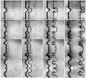
The Schlieren images of the shocked multi-mode interface for large- $w_0$ cases are shown in figure 3. The interface morphologies in large-
 $w_0$ cases are qualitatively similar to the corresponding small-
 $w_0$ ones. However, for the large-
 $w_0$ cases, there is a greater misalignment between the pressure gradient of the shock wave and the density gradient of the interface, resulting in more baroclinic vorticity production and the earlier appearance of vortices. Besides, at late time in the k
 $_2$AP case (1062
  $\mathrm {\mu }$s), the spike structures on the multi-valued interface break, and the whole interface becomes chaotic, which indicates that the transition may occur earlier when the initial interface amplitude is larger (Mohaghar et al. Reference Mohaghar, Carter, Pathikonda and Ranjan2019; Mansoor et al. Reference Mansoor, Dalton, Martinez, Desjardins, Charonko and Prestridge2020).

Figure 3. Schlieren images of the multi-mode interface evolution for large- $w_0$ cases.
The captured interface morphology is distinct such that the interface contours in all cases can be extracted by an image processing program, as indicated by the insets in figures 4 and 5. The mean  $y$ coordinate in each image is taken as the average position of the local interface. Spectrum analysis is then performed on the averaged interface contour before the interface becomes multi-valued, and the amplitudes of three constituent modes are acquired, as shown in figures 4 and 5. Time is normalized as
  $\tau _{n}=k_1|v_{k_n}^{R}|t$, where
  $v_{k_n}^{R}$ is the Richtmyer growth rate of mode
  $k_n$ calculated by the impulsive theory (Richtmyer Reference Richtmyer1960):
 \begin{equation} v_{k_n}^{R}=Z_ckA^{+}{\rm \Delta} va_{k_n}^{0}\cos(\phi_{k_n}), \end{equation}
in which  $Z_c$ (
 $=1-{\rm \Delta} v/v_s$) is the shock compression factor and is equal to 0.84 in all cases. In the present coordinate system,
  $v_{k_n}^{R}$ is positive if
  $\phi _{k_n}$ = 0, but becomes negative if
  $\phi _{k_n}={\rm \pi}$. The amplitude is scaled as
  $\eta _n=k_1|a_{k_n}(t)-Z_ca_{k_n}^{0}\cos (\phi _{k_n})|$, with
  $a_{k_n}(t)$ the time-varying amplitude of mode
  $k_n$.

Figure 4. The dimensionless amplitudes of three constituent modes obtained from small- $w_0$ cases. The insets show the interface contours for the spectrum analysis in which numbers indicate time in
  $\mathrm {\mu }$s. Run1 and run2 represent typical experimental runs. The black dashed line represents the impulsive theory (Richtmyer Reference Richtmyer1960). The coloured solid lines, dashed lines and dash-dotted lines represent the amplitudes of three constituent modes calculated by the Haan-RM model (3.4), the Ofer-RM model (3.7) and the present model (3.10), respectively, and similarly hereinafter.

Figure 5. The dimensionless amplitudes of three modes obtained from large- $w_0$ cases.
In small- $w_0$ cases, as shown in figure 4, it is clear that the dimensionless amplitudes of modes
  $k_1$ and
  $k_2$ are larger than those of mode
  $k_3$ in IP-s and AP-s cases, but smaller than those of mode
  $k_3$ in k
 $_3$AP and k
 $_2$AP cases. In other words, the low-order modes (modes
  $k_1$ and
  $k_2$) in IP-s and AP-s cases dominate the flow, whereas the high-order mode (mode
  $k_3$) in k
 $_3$AP and k
 $_2$AP cases dominates the flow, which agree with the observations in figure 2. For example, in the IP-s case in figure 2(a), the late-time interface is dominated by long-wavelength structures (a large bubble and two groups of large and small spikes), but in the k
 $_3$AP case in figure 2(b), the late-time interface is dominated by four short-wavelength structures (four pairs of spikes and bubbles). Therefore, the mode-competition effect plays a role in the amplitude development of the constituent modes in early stages. Since the small perturbation hypothesis is satisfied for each constituent mode, the impulsive theory should be valid to predict the amplitude growth of each constituent mode if the mode-competition effect is ignored. However, compared with the predictions of the impulsive theory, in the IP-s case, mode
  $k_1$ development is promoted but mode
  $k_3$ development is suppressed, while mode
  $k_2$ development is not obviously influenced by the mode-competition effect. Differently, in the k
 $_3$AP-s case, the developments of both modes
  $k_1$ and
  $k_2$ are suppressed, while the development of mode
  $k_3$ is not obviously influenced by the mode-competition effect. Therefore, the mode-competition effect is greatly influenced by the initial wavenumber and the initial phase of the constituent mode.
In large- $w_0$ cases, as shown in figure 5, similar to the corresponding small-
 $w_0$ cases, the amplitudes of both modes
  $k_1$ and
  $k_2$ are larger than those of mode
  $k_3$ in IP-h and AP-h cases, but smaller than those of mode
  $k_3$ in k
 $_3$AP-h and k
 $_2$AP-h cases. However, compared with the impulsive theory, mode
  $k_2$ development in the IP-h case is suppressed whereas mode
  $k_3$ development in the k
 $_3$AP-h case is promoted by the mode-competition effect, which is different from the results of corresponding small-
 $w_0$ cases. Therefore, the initial amplitude of the constituent mode also affects the mode-competition effect. In summary, the effect of mode competition is closely related to the initial spectra, including the wavenumber, the phase and the initial amplitude of the constituent modes.
Generally, the linear stage is defined by the fact that Fourier modes evolve separately (Drazin & Reid Reference Drazin and Reid2004; Chandrasekhar Reference Chandrasekhar2013). Because it is difficult to obtain the starting point of the linear stage in reality, usually used within the framework of RM instability is that the linear stage occurs as long as mode  $k$ satisfies
  $a_{k}(t)k<\alpha$. This constant
  $\alpha$ depends essentially on the accuracy required. As a result, it is generally accepted that the necessary condition of the linear RM instability is
  $a_{k}^{0}k\ll 1$ (Mügler & Gauthier Reference Mügler and Gauthier1998; Collins & Jacobs Reference Collins and Jacobs2002; Mikaelian Reference Mikaelian2003; Niederhaus & Jacobs Reference Niederhaus and Jacobs2003; Mariani et al. Reference Mariani, Vandenboomgaerde, Jourdan, Souffland and Houas2008; Vandenboomgaerde et al. Reference Vandenboomgaerde, Souffland, Mariani, Biamino, Jourdan and Houas2014; Mansoor et al. Reference Mansoor, Dalton, Martinez, Desjardins, Charonko and Prestridge2020). However, the linear stage still exists for a very large initial
  $a_{k}^{0}k$ at the expense of a large reduction in the duration of the linear stage (Rikanati et al. Reference Rikanati, Oron, Sadot and Shvarts2003; Dell, Stellingwerf & Abarzhi Reference Dell, Stellingwerf and Abarzhi2015; Zhai et al. Reference Zhai, Dong, Si and Luo2016; Dell et al. Reference Dell, Pandian, Bhowmick, Swisher, Stanic, Stellingwerf and Abarzhi2017). It should be noted that there are harmonics growing with time in these large initial
  $\alpha$ cases but they are (almost) negligible. Therefore, this linear stage within large initial
  $\alpha$ is actually a quasi-linear stage. As listed in table 2, the criterion of dimensionless time, i.e.
  $\tau _n^{*}$ (
 $=k_n|v_{k_n}^{R}|t$), of mode
  $k_n$ between the quasi-linear stage and the nonlinear stage is evaluated from experiments. It is found that
  $\tau _n^{*}$ of the three initial modes are less than the generally accepted criterion of dimensionless time of 0.7 for the single-mode RM instability (Niederhaus & Jacobs Reference Niederhaus and Jacobs2003), indicating that the large initial
  $a_{k_n}^{0}k_n$ results in a very short quasi-linear stage and the mode competition advances the nonlinearity of the multi-mode RM instability.
Table 2. The criterion of dimensionless time ( $\tau _n^{*}$) of mode
  $k_n$ between the quasi-linear stage and the nonlinear stage.

3.2. Linear and nonlinear theories
To quantitatively describe the 2-D multi-mode RM instability development, linear and nonlinear theories based on the impulsive theory, the modal model and the interpolation model have been established.
I. Impulsive theory. If each mode of a multi-mode interface satisfies  $|a_k(t)k|\ll 1$, the whole interface evolves linearly. Previous studies (Sadot et al. Reference Sadot, Erez, Alon, Oron, Levin, Erez, Ben-Dor and Shvarts1998; Mikaelian Reference Mikaelian2005; Di Stefano et al. Reference Di Stefano, Malamud, Kuranz, Klein and Drake2015a,Reference Di Stefano, Malamud, Kuranz, Klein, Stoeckl and Drakeb; Liang et al. Reference Liang, Zhai, Ding and Luo2019) considered that the mode-competition effect is negligible in quasi-linear stages. Therefore, for an initial light–heavy interface, the linear amplitude growth rate (
 $v_k^{l}$) of mode
  $k$ can be described by the impulsive theory (3.1), i.e.
  $v_k^{l}=v_k^{R}$. For an initial heavy–light perturbed interface, the Richtmyer growth rate should be modified as
  $v_k^{R}=(Z_c+1)kA^{+}{\rm \Delta} va_{k}^{0}\cos (\phi _{k})/2$ (Meyer & Blewett Reference Meyer and Blewett1972).
When  $a_k^{0}$ is comparable to its wavelength or/and the shock intensity is large, the high-amplitude effect or/and the high-Mach-number effect will inhibit
  $v_k^{R}$ (Rikanati et al. Reference Rikanati, Oron, Sadot and Shvarts2003; Dell et al. Reference Dell, Stellingwerf and Abarzhi2015, Reference Dell, Pandian, Bhowmick, Swisher, Stanic, Stellingwerf and Abarzhi2017; Guo et al. Reference Guo, Zhai, Ding, Si and Luo2020). Here, the high-amplitude effect and the high-Mach-number effect are considered independently. Then the modified Richtmyer growth rate (
 $v_k^{MR}$) is
 \begin{equation} v_k^{MR}=\beta{\rm \Delta} v\,\mathrm{tanh}(R_kv_k^{R}/\beta{\rm \Delta} v), \end{equation}
where  $R_k$ (
 $=1/[1+(ka_k^{0}/3)^{(4/3)}]$) is the reduction factor proposed by Dimonte & Ramaprabhu (Reference Dimonte and Ramaprabhu2010) to quantify the high-amplitude effect on mode
  $k$. For small-
 $w_0$ cases,
  $R_{k_1}=0.97$,
  $R_{k_2}=0.93$ and
  $R_{k_3}=0.91$; for large-
 $w_0$ cases,
  $R_{k_1}=0.91$,
  $R_{k_2}=0.88$ and
  $R_{k_3}=0.91$. Parameter
  $\beta$ (
 $=1-{\rm \Delta} v/v_t$) is the reduction factor proposed by Hurricane et al. (Reference Hurricane, Burke, Maples and Viswanathan2000) to quantify the high-Mach-number effect on all modes, and
  $\beta =0.64$ in all cases.
II. Modal model. When the mode competition starts to play a role, the interface evolution enters the early nonlinear stage. Haan (Reference Haan1991) first proposed a modal model applicable to the 2-D RT instability, and then deduced the modal model for the 2-D RM instability with zero acceleration ( $g=0$) and assuming
  $|a_k(t)|\gg |a_k^{0}|$, i.e. ignoring the initial amplitude terms, as
 \begin{equation} a_k(t)=a_k^{l}(t)+\frac{1}{2}Ak\sum_{k'}a_{k'}^{l}(t)a_{k''}^{l}(t)\times \left(\frac{1}{2}-\hat{\boldsymbol{k}}\boldsymbol{\cdot}\widehat{\boldsymbol{k'}}-\frac{1}{2} \widehat{\boldsymbol{k'}}\boldsymbol{\cdot}\widehat{\boldsymbol{k''}}\right), \end{equation}
where  $\boldsymbol {k''}=\boldsymbol {k}-\boldsymbol {k'}$;
  $\boldsymbol {k}$,
  $\boldsymbol {k'}$ and
  $\boldsymbol {k''} \in \mathbb {R}^{2}$; and
  $\hat {\boldsymbol {k}}$ is the unit vector
  $\boldsymbol {k}$/
 $k$. Amplitude
  $a_k^{l}(t)$ is the linear amplitude of mode
  $k$. Taking the first derivative of (3.3) and using the post-shock physical parameters, the ‘Haan-RM’ model can be obtained to calculate the early nonlinear amplitude growth rate
  $v_k^{en}(t)$ of mode
  $k$ as
 \begin{equation} v_k^{en}(t)=v_k^{MR}+A^{+}k \left(2\sum_{k'}v_{k'}^{MR}v_{k+k'}^{MR}-\sum_{k'< k}v_{k'}^{MR}v_{k-k'}^{MR}\right)t, \end{equation}
where  $k$,
$k$,  $k'$ and
  $k''\in \mathbb {R}^{+}$. The first term on the right-hand of the Haan-RM model indicates that the development of each mode of a multi-mode RM unstable interface is still strongly influenced by its independent perturbation growth. At
  $t\approx 0$, the Haan-RM model reduces to
  $v_k^{en}(t)\approx v_k^{l}=v_k^{MR}$, which indicates that the mode-competition effect is very weak and can be ignored. The second term on the right-hand side is the mode-competition term, and it is evident that as
  $t$ increases, the mode-competition effect plays a more important role in influencing the RM instability. The first sum term in the mode-competition term represents the generation of mode
  $k$ from high-order modes and indicates the bubble-merging process. The second sum term in the mode-competition term represents the generation of mode
  $k$ from the interaction of low-order modes, which is related to the bubble-spike asymmetry and the total mixing rate decrement.
However, the initial amplitude terms cannot be ignored in deducing the modal model for the whole process of the RM instability, especially when the initial amplitude of mode  $k$ is large. Now, the modal model for the RM instability including the initial amplitude terms is re-derived. Based on the modal model solved by Ofer et al. (Reference Ofer, Alon, Shvarts, McCrory and Verdon1996) to second-order accuracy with
  $g=\mathrm {constant}$ for the RT instability,
 \begin{equation} a_k(t)=a_k^{l}(t)+\frac{1}{2}Ak\left[\sum_{k'}a_{k'}^{l}(t)a_{k+k'}^{l}(t)-\frac{1}{2} \sum_{k'< k}a_{k'}^{l}(t)a_{k-k'}^{l}(t)\right], \end{equation}
we take the second derivative of (3.5) with time, and get
 \begin{align} \frac{\mathrm{d}^{2}a_{k}(t)}{\mathrm{d}t^{2}}&=Agka_{k}^{0}+ \frac{1}{2}A^{2}gk\left\{\sum_{k'}[k'a_{k'}^{0}a_{k+k'}^{l}(t)+2 \sqrt{k'(k+k')}a_{k'}^{0}a_{k+k'}^{0} \right.\nonumber\\ &\quad +(k+k')a_{k+k'}^{0}a_{k'}^{l}(t)]-\frac{1}{2}\sum_{k'< k}[k'a_{k'}^{0}a_{k-k'}^{l}(t) \nonumber\\ &\quad \left.\vphantom{\sum_{k'}} +2\sqrt{k'(k-k')}a_{k'}^{0}a_{k+k'}^{0}+(k-k')a_{k-k'}^{0}a_{k'}^{l}(t)]\right\}. \end{align}
Similar to Richtmyer (Reference Richtmyer1960), the constant  $g$ is replaced by an impulsive acceleration
  $\delta t{\rm \Delta} v$ (
 $\delta t=0$ when
  $t=0$ and
  $\delta t=1$ when
  $t>0$) and the post-shock physical parameters are adopted. Through integrating (3.6) with time,
  $v_{k}^{en}$ for the RM instability can be expressed as a superposition of the linear amplitude growth rate
  $v_k^{l}$ and the weakly nonlinear modification
  $v_k^{wn}(t)$:
 \begin{equation} v_k^{en}(t)=v_k^{l}+v_k^{wn}(t), \end{equation}
with
 \begin{align} v_k^{l}&=v_k^{MR}+\frac{1}{2}A^{+}k\left\{\sum_{k'} \left[v_{k'}^{MR}Z_ca_{k+k'}^{0}+v_{k+k'}^{MR}Z_ca_{k'}^{0}\left(1+2\sqrt{\frac{k}{k'}+1}\right)\right]\right. \nonumber\\ &\quad \left.-\frac{1}{2}\sum_{k'< k}\left[v_{k'}^{MR}Z_ca_{k-k'}^{0}+v_{k-k'}^{MR}Z_ca_{k'}^{0} \left(1+2\sqrt{\frac{k}{k'}-1}\right)\right]\right\} \end{align}
and
 \begin{equation} v_k^{wn}(t)=A^{+}k\left(\sum_{k'}v_{k'}^{MR}v_{k+k'}^{MR}-\frac{1}{2} \sum_{k'< k}v_{k'}^{MR}v_{k-k'}^{MR}\right)t. \end{equation}
Here, (3.7)–(3.9) are called the ‘Ofer-RM’ model. Different from  $v_k^{l}=v_k^{MR}$ indicated by the Haan-RM model,
  $v_k^{l}$ in the Ofer-RM model is a superposition of
  $v_k^{MR}$ with the mode-competition term that is related to the initial amplitudes of constituent modes. In other words, the mode-competition effect influences each mode perturbation growth in the quasi-linear stage of the multi-mode RM instability, which is different from the previous view that the mode-competition effect can be ignored in the quasi-linear stage (Sadot et al. Reference Sadot, Erez, Alon, Oron, Levin, Erez, Ben-Dor and Shvarts1998; Mikaelian Reference Mikaelian2005; Di Stefano et al. Reference Di Stefano, Malamud, Kuranz, Klein and Drake2015a,Reference Di Stefano, Malamud, Kuranz, Klein, Stoeckl and Drakeb; Liang et al. Reference Liang, Zhai, Ding and Luo2019). Besides, when
  $v_k^{en}(t)=0$, mode
  $k$ is fully saturated. Here, additional rules introduced by Ofer et al. (Reference Ofer, Alon, Shvarts, McCrory and Verdon1996) for the enforced post-saturation treatment in calculating
  $v_k^{en}(t)$ are adopted: (i) no weakly nonlinear modifications of a saturated mode to low-order modes and (ii) the phases of the harmonics generated by the saturated modes are opposite.
The predictions from the Haan-RM model and the Ofer-RM model are calculated as shown in figures 4 and 5. For small- $w_0$ cases, because the initial amplitudes of three modes are small, both models give reasonable predictions of the experimental results. Differently, for large-
 $w_0$ cases, the Ofer-RM model provides a better prediction of the amplitude growth than the Haan-RM model for some constituent modes, such as modes
  $k_1$ and
  $k_3$ in the IP-h case, mode
  $k_1$ in the k
 $_2$AP-h case and modes
  $k_1$ and
  $k_2$ in the AP-h case. Note that the amplitude developments of mode
  $k_1$ in the IP-h case and mode
  $k_3$ in the AP-h case deviate from predictions of the impulsive theory from the very beginning, which verifies that the mode-competition effect plays an important role in the early evolution of a multi-mode interface. In summary, the Ofer-RM model is more applicable to describing the multi-mode RM instability behaviour in the early nonlinear stage, especially when the initial amplitudes of constituent modes are large. Meanwhile, the present experimental results prove that the linear growth of each mode amplitude is also influenced by the mode-competition effect.
Based on (3.8),  $v_k^{l}$ considering the mode-competition effect is calculated and compared with
  $v_k^{MR}$ without the mode-competition effect, as listed in table 3 for all cases. The difference between
  $v_k^{l}$ and
  $v_k^{MR}$ is larger in large-
 $w_0$ cases than in small-
 $w_0$ cases. According to the modal analysis (Haan Reference Haan1991; Ofer et al. Reference Ofer, Alon, Shvarts, McCrory and Verdon1996; Miles et al. Reference Miles, Edwards, Blue, Hansen, Robey, Drake, Kuranz and Leibrandt2004), the coupling of constituent modes will generate new harmonics. In our experiments,
  $k_2$ and
  $k_3$ are integral multiples of
  $k_1$, and thus no modes with wavenumber lower than
  $k_1$ will be generated (Miles et al. Reference Miles, Edwards, Blue, Hansen, Robey, Drake, Kuranz and Leibrandt2004). However, three new harmonics with higher order, i.e. harmonics
  $k_4$ (
 $=k_1+k_3$),
  $k_5$ (
 $=k_2+k_3$) and
  $k_6$ (
 $=k_3+k_3$), are generated if only the first generation of new harmonics is considered (Ofer et al. Reference Ofer, Alon, Shvarts, McCrory and Verdon1996). The values of
  $v_k^{l}$ for the three generated harmonics are listed in table 3. It is evident that the new generated harmonics cannot be ignored in the multi-mode RM instability development in early stages.
Table 3. Comparison of the modified Richtmyer growth rate ( $v_{k_n}^{MR}$) calculated by (3.2) with the linear amplitude growth rate (
 $v_{k_n}^{l}$) calculated by (3.7). The unit for the growth rate is m s
 $^{-1}$.

III. Interpolation model. Although the Ofer-RM model generally gives a better prediction than the Haan-RM model in large- $w_0$ cases, it still underestimates mode
  $k_2$ development in the k
 $_3$AP-s case and overestimates mode
  $k_2$ development in the AP-h case when
  $t$ is large. According to the Ofer-RM model, when
  $t\rightarrow \infty$,
  $v_k^{l}$ is neglected and
  $v_k^{en}$ is proportional to
  $t$ as long as
  $v_k^{wn}$ is non-zero. Actually, in the consideration of classical single-mode RM instability, the late nonlinear amplitude growth rate (
 $v^{ln}_k$) of mode
  $k$ should be
  $t^{-1}$ decay (Hecht, Alon & Shvarts Reference Hecht, Alon and Shvarts1994; Alon et al. Reference Alon, Hecht, Ofer and Shvarts1995; Mikaelian Reference Mikaelian1998) because of the suppression of high-order (three orders or greater) harmonics generated by mode
  $k$ itself (Velikovich & Dimonte Reference Velikovich and Dimonte1996; Zhang & Sohn Reference Zhang and Sohn1997; Nishihara et al. Reference Nishihara, Wouchuk, Matsuoka, Ishizaki and Zhakhovsky2010; Velikovich, Herrmann & Abarzhi Reference Velikovich, Herrmann and Abarzhi2014). In the multi-mode RM instability counterparts, the perturbation width growth in the fully turbulent stage is proportional to
  $t^{\theta }$ as a result of bubble merging (Alon et al. Reference Alon, Hecht, Mukamel and Shvarts1994, Reference Alon, Hecht, Ofer and Shvarts1995). Although the value of
  $\theta$ has not been unified, it should be much lower than 1.0, as reviewed by Zhou (Reference Zhou2017a,Reference Zhoub). Therefore, the perturbation width growth rate of a multi-mode interface should be proportional to
  $t^{\theta -1}$ with
  $-1<(\theta -1)<0$ in the fully turbulent stage. As a result, the Ofer-RM model with second-order accuracy is not applicable to describing the late-time 2-D multi-mode RM instability, and its scope should be extended by considering the suppression from high-order harmonics.
An interpolation model proposed by Dimonte & Ramaprabhu (Reference Dimonte and Ramaprabhu2010) (DR model) for predicting 2-D single-mode amplitude growth covers the entire time domain from the early to late nonlinear stages of the RM instability, and it has been well verified by several independent experiments (Dimonte et al. Reference Dimonte, Frerking, Schneider and Remington1996; Sadot et al. Reference Sadot, Erez, Alon, Oron, Levin, Erez, Ben-Dor and Shvarts1998; Niederhaus & Jacobs Reference Niederhaus and Jacobs2003; Jacobs & Krivets Reference Jacobs and Krivets2005) through considering diverse amplitude-to-wavelength ratios, shock intensities and density ratios. In this work, the scope of the Ofer-RM model is extended in combination with the DR model, and then  $v^{ln}_k$ can be expressed as an average of the bubble amplitude growth rate
  $v_{kb}^{ln}(t)$ with the spike amplitude growth rate
  $v_{ks}^{ln}(t)$ of mode
  $k$:
$k$:
 \begin{equation} v_k^{ln}(t)=\tfrac{1}{2}[v_{kb}^{ln}(t)+v_{ks}^{ln}(t)], \end{equation}
with
 \begin{equation} \left.\begin{gathered} v_{kb/ks}^{ln}(t)=v_k^{en}(t)\frac{1+(1\mp|A^{+}|)|kv_k^{en}(t)t|}{1+C_{b/s}|kv_k^{en} (t)t|+(1\mp|A^{+}|)F_{b/s}|kv_k^{en}(t)t|^{2}},\\ C_{b/s}=\frac{4.5\pm|A^{+}|+(2\mp|A^{+}|)(ka_0^{k})}{4},\quad F_{b/s}=1\pm|A^{+}|. \end{gathered}\right\} \end{equation}
Finally, (3.2), (3.7) and (3.10) constitute the ‘present’ model for describing the 2-D multi-mode RM instability in this work. Notably, the self-similar law shows that the perturbation width growth rate of a multi-mode interface in the fully turbulent stage has a  $t^{\theta -1}$ dependence and therefore approaches zero when
  $t\rightarrow \infty$. According to (3.10) and (3.11), when
  $t\rightarrow \infty$,
  $v_k^{ln}(t)$ also approaches zero but shows a
  $t^{-1}$ dependence, i.e.
  $\theta =0$, which violates the self-similar law. However, the
  $t^{-1}$ asymptotic dependence agrees with the potential model (Alon et al. Reference Alon, Hecht, Mukamel and Shvarts1994, Reference Alon, Hecht, Ofer and Shvarts1995; Oron et al. Reference Oron, Arazi, Kartoon, Rikanati, Alon and Shvarts2001), the vortex model (Rikanati et al. Reference Rikanati, Alon and Shvarts1998) and recent experimental findings (Mansoor et al. Reference Mansoor, Dalton, Martinez, Desjardins, Charonko and Prestridge2020).
The predictions of the present model for our experiments are shown in figures 4 and 5, and a good agreement between them is achieved. Besides, data from literature are extracted to validate the present model. First, the numerical results from figures 9 and 10 of Vandenboomgaerde et al. (Reference Vandenboomgaerde, Gauthier and Mügler2002) with both  $M$ (
$M$ ( $= 1.0962$) and
  $A^{+}$ (
 $= 0.764$) similar to those in our experiments are extracted, as shown in figure 6(a). The initial interface consists of three modes:
  $a_{k_1}^{0}=0.35\times 10^{-3}$,
  $a_{k_2}^{0}=1.9055\times 10^{-3}$ and
  $a_{k_3}^{0}=1.072\times 10^{-3}$ m;
  $k_1=274.855\,\textrm {m}^{-1}$,
  $k_2=3k_1/7$ and
  $k_3=4k_1/7$. For the data in figure 9 of Vandenboomgaerde et al. (Reference Vandenboomgaerde, Gauthier and Mügler2002),
  $\phi _1=\phi _2=\phi _3=0$, while for the data in figure 10,
  $\phi _1=\phi _2=\phi _3={\rm \pi}$. For these two cases,
  $R_{k_1}=0.97$,
  $R_{k_2}=0.93$ and
  $R_{k_3}=0.95$;
  $\beta =0.80$. It is found that the predictions of the present model agree well with all the numerical results (Vandenboomgaerde et al. Reference Vandenboomgaerde, Gauthier and Mügler2002). Further, the experimental and numerical results (Di Stefano et al. Reference Di Stefano, Malamud, Kuranz, Klein, Stoeckl and Drake2015b) with a much larger
  $M$ (
$M$ ( $= 8$) and a smaller
  $A^{+}$ (
 $= 1/3$) compared with our experimental conditions are predicted by the present model. The initial interface in the literature (Di Stefano et al. Reference Di Stefano, Malamud, Kuranz, Klein, Stoeckl and Drake2015b) consists of two modes:
  $a_{k_1}^{0}=5\times 10^{-6}$ m,
  $a_{k_2}^{0}=0.5a_{k_1}^{0}$;
  $k_1=6.28\times 10^{4}\,\textrm {m}^{-1}$,
  $k_2=2k_1$;
  $\phi _1=0$,
  $\phi _2={\rm \pi}$;
  $R_{k_1}=0.91$,
  $R_{k_2}=0.91$;
  $\beta =0.35$. The amplitude growths of the two constituent modes and the harmonic
  $k_3$ generated by the coupling of modes
  $k_1$ and
  $k_2$ are extracted from figure 5 of Di Stefano et al. (Reference Di Stefano, Malamud, Kuranz, Klein, Stoeckl and Drake2015b), as shown in figure 6(b). It is found that not only the constituent mode amplitudes, but also the generated new harmonic amplitude are well predicted by the present model. Overall, the present model established in this work by considering both the mode-competition effect and the high-order harmonics effect is applicable to the nonlinear RM instability before the transition.

Figure 6. The amplitudes of modes obtained from (a) the numerical results in Vandenboomgaerde et al. (Reference Vandenboomgaerde, Gauthier and Mügler2002) and (b) the experimental and numerical results in Di Stefano et al. (Reference Di Stefano, Malamud, Kuranz, Klein, Stoeckl and Drake2015b). Coloured lines represent the predictions calculated with the present model.
3.3. The perturbation width growth
The memory of the perturbation width growth of a multi-mode interface on its initial spectrum is crucial to RM instability research. The perturbation width  $w(t)$ of a multi-mode interface is defined as the streamwise distance from the upstream point (UP) to the downstream point (DP) of an interface, as shown in figure 2(b). The variations of the perturbation width measured from the schlieren images for small- and large-
 $w_0$ cases are shown in figures 7(a) and 8(a), respectively. The time is normalized as
  $\tau _w=0.5k_1v_w^{MR}t$, where
  $v_w^{MR}=\sum _{1}^{3}v_{k_n}^{MR}[\cos (k_nx_{DP})-\cos (k_nx_{UP})]$, with
  $x_{UP}$ and
  $x_{DP}$ being the
  $x$ coordinates of UP and DP, respectively. The half of the perturbation width is scaled as
  $\eta _w=0.5k_1[w(t)-Z_cw^{0}]$. To compare the perturbation width between the multi-mode interface and the classical single-mode interface, the predictions from the impulsive theory and the DR model are calculated, as shown in figures 7(a) and 8(a), respectively. It is evident that the perturbation width growth of a multi-mode interface in the early stage (
 $\tau _w\leq 0.5$) is close to or even larger than the single-mode linear growth, which indicates that the mode-competition effect may enhance the initial growth of the multi-mode perturbation. Later, the perturbation width growth in all cases is smaller than the single-mode linear growth when
  $\tau _w>0.7$ and smaller than the single-mode nonlinear growth when
  $\tau _w>1.2$. Therefore, the mode-competition effect suppresses the multi-mode interface development at late stages because it enhances local mixing and reduces the global mixing. Besides, the
  $w(t)$ growth curves in all cases deviate from each other, which indicates that the initial spectrum influences the 2-D multi-mode RM instability until the late nonlinear stage.

Figure 7. Comparison of the perturbation width (a), growth rate of the perturbation width (b), widths of bubble and spike (c) and width growth rates of bubble and spike (d) in small- $w_0$ cases. Black dashed lines and dash-dotted lines represent the single-mode linear and nonlinear amplitude growth rates calculated by the impulsive theory (Richtmyer Reference Richtmyer1960) and DR model (Dimonte & Ramaprabhu Reference Dimonte and Ramaprabhu2010), respectively. Coloured solid lines represent the predictions from the sum model calculated with (3.12), and similarly hereinafter.

Figure 8. Comparison of the perturbation width (a), growth rate of the perturbation width (b), widths of bubble and spike (c) and width growth rates of bubble and spike (d) in large- $w_0$ cases.
To more clearly distinguish the differences of the perturbation growth with diverse initial conditions, through the direct differentiation of the experimental data, the perturbation width growth rate  $\dot {w}(t)$ of a multi-mode interface is acquired, and compared with the single-mode linear and nonlinear amplitude growth rates, as shown in figures 7(b) and 8(b) for all cases. The perturbation width growth rate is scaled as
  $\zeta _w=\dot {w}_s(t)/v_w^{MR}$. Therefore, the dimensionless single-mode linear growth rate is
  $\zeta _w=1$. In small-
 $w_0$ cases,
  $\dot {w}(t)$ in IP-s and AP-s cases is smaller than that of the single-mode growth rate during the whole process. The value of
  $\dot {w}(t)$ in k
 $_{3}$AP-s and k
 $_{2}$AP-s cases is larger than that of the single-mode counterpart in early times (
 $\tau _w\leq 0.5$), but smaller than that of the single-mode counterpart in late stages. In large-
 $w_0$ cases, differently,
  $\dot {w}(t)$ in IP-h and k
 $_2$AP-h cases is smaller than that of the single-mode growth rate during the whole process. The value of
  $\dot {w}(t)$ in k
 $_{3}$AP-h and AP-h cases is larger than that of the single-mode counterpart in early times (
 $\tau _w\leq 0.5$), but smaller than that of the single-mode counterpart in late stages. Therefore, both the phase and amplitude of the constituent modes influence the mode-competition effect on the perturbation width growth of a multi-mode interface. Besides, the growth rate of a multi-mode interface with all modes in-phase is smaller than the counterpart in the classical single-mode case and other multi-mode cases. In addition, under specific conditions, such as in k
 $_{3}$AP-s and k
 $_{3}$AP-h cases, the mode-competition effect promotes the perturbation width growth in early stages.
Compared with the reference moving with the post-shock flow velocity, the width growths of the bubble ( $w_b(t$)) and the spike (
 $w_s(t$)) are separated, as shown in figures 7(c) and 8(c) for small- and large-
 $w_0$ cases, respectively. The bubble/spike width is scaled as
  $\eta _{b/s}=k_1[w_{b/s}(t)-Z_cw_{0b/0s}^{0}]$, in which
  $w_{0b/0s}$ is the initial bubble/spike width, as listed in table 1. The bubble width of the multi-mode interface in all cases is lower than that of the single-mode counterpart in late stages (
 $\tau _w\leq 0.5$), which indicates that the mode-competition effect advances the saturation of the bubble evolution in the 2-D multi-mode RM instability. The nonlinear behaviour of the spike of a multi-mode interface is greatly influenced by the initial spectra. In small-
 $w_0$ cases,
  $w_s(t)$ in IP-s and AP-s cases are lower while
  $w_s(t)$ in k
 $_2$AP-s and k
 $_3$AP-s cases are higher than those of the single-mode counterpart, which means that the phase of the constituent mode influences the spike behaviour in the 2-D multi-mode RM instability. In large-
 $w_0$ cases,
  $w_s(t)$ in k
 $_3$AP-h, k
 $_2$AP-h and AP-h cases are close to those of the single-mode counterpart, which indicates that the initial amplitude of the constituent mode influences the spike behaviour. The width growth rates of the bubble
  $\dot {w}_b(t)$ and the spike
  $\dot {w}_s(t)$ are calculated, as shown in figures 7(d) and 8(d) for small- and large-
 $w_0$ cases, respectively. The bubble/spike width growth rate is scaled as
  $\zeta _{b/s}=2\dot {w}_{b/s}(t)/v_w^{MR}$. It is shown that the bubble width growth rate of a multi-mode interface is generally lower than that of the single-mode counterpart. The spike width growth rate reflects whether the mode-competition effect promotes or suppresses the multi-mode RM instability in early stages.
Since the angle between the incident shock and UP (DP) is zero, no vorticity is deposited at UP (DP). Therefore, UP and DP on the interface remain single-valued until the late nonlinear stage before the transition. As a result, the perturbation width growth of a multi-mode interface can be predicted by superimposing the perturbation growths of initially constituent modes and the generated harmonics at  $x_{UP}$ and
  $x_{DP}$. In the present coordinate system, the time-varying
  $w(t)$ growth is superimposed by
  $w_b(t)$ and
  $w_s(t)$:
 \begin{equation} w(t)=w_b(t)+w_s(t), \end{equation}
with
 \begin{gather} w_b(t)=Z_cw_{0b}+\sum_{n}\int_{0}^{t}v_{k_n}^{ln}\cos(k_nx_{\mathrm{DP}})\,\mathrm{d}t, \end{gather}
 \begin{gather}w_s(t)=Z_cw_{0s}-\sum_{n}\int_{0}^{t}v_{k_n}^{ln}\cos(k_nx_{\mathrm{UP}})\, \mathrm{d}t. \end{gather}
In this work, (3.12)–(3.14) constitute the ‘sum’ model which is used to calculate the perturbation width by superimposing the amplitudes of three constituent modes and three generated harmonics. By linear fitting of the perturbation width of a multi-mode interface before 120  $\mathrm {\mu }$s in all cases, the experimental initial perturbation width growth rate (
 $\dot {w}_{exp}^{0}$) can be obtained, as listed in table 4. The theoretical initial perturbation width growth rate of the interface (
 $\dot {w}_{theo}^{0}$) can be evaluated by superimposing the amplitude growth rates of three constituent modes and three generated harmonics:
 \begin{equation} \dot{w}_{theo}^{0}=\sum_{n=1}^{6}v_{k_n}^{ln}[\cos(k_nx_{\mathrm{DP}})-\cos(k_nx_{\mathrm{UP}})]. \end{equation}
The values of  $\dot {w}_{theo}^{0}$ in all cases are listed in table 4 and agree well with the experimental results. Then, the predictions of the sum model for
  $w(t)$,
  $w_b(t)$ and
  $w_s(t)$ are shown in figures 7 and 8, and agree well with the experimental counterparts. Meanwhile, the differentiation of the sum model is calculated and compared with the experimental
  $\dot {w}(t)$,
  $\dot {w}_b(t)$ and
  $\dot {w}_s(t)$, and a good agreement is also achieved between them. Note that there are several break points, for example in k
 $_3$AP-h and AP-h cases, when the sum model is used to predict the growth rates, which is ascribed to the enforced post-saturation treatment adopted when
  $v_k^{en}$ is calculated. After the incident shock wave impacts the interface, the transverse waves between the transmitted shock and reflected shock interact with the interface, especially when the initial interface perturbation is prominent. Therefore, the non-uniform flow influences the linear interface growth (Guo et al. Reference Guo, Zhai, Ding, Si and Luo2020), resulting in the perturbation width growth varying around the sum model prediction at an early regime.
Table 4. Comparison of the experimental initial perturbation width growth rate ( $\dot {w}_{exp}$) of the multi-mode interface with the theoretical counterpart (
 $\dot {w}_{theo}$) calculated with (3.15).

To further validate the sum model, the experimental results with  $M$ (
$M$ ( $= 1.3$) and
  $A^{+}$ (
 $= 0.67$) similar to our experiments extracted from figure 4(a) in Sadot et al. (Reference Sadot, Erez, Alon, Oron, Levin, Erez, Ben-Dor and Shvarts1998) are adopted as shown in figure 9(a). The initial interface is a two-bubble interface, which is dominated by the first five order modes:
  $a_{k_1}^{0}=1.49\times 10^{-3}$,
  $a_{k_2}^{0}=1.06\times 10^{-3}$,
  $a_{k_3}^{0}=0.40\times 10^{-3}$,
  $a_{k_4}^{0}=0.21\times 10^{-3}$,
  $a_{k_5}^{0}=0.10\times 10^{-3}$ m;
  $k_1=180\,\textrm {m}^{-1}$,
  $k_i=ik_1$ with
  $i=2$–
 $5$;
$5$;  $\phi _1={\rm \pi}$,
  $\phi _2=\phi _3=\phi _4=\phi _5=0$;
  $R_{k_1}=0.92$,
  $R_{k_2}=0.89$,
  $R_{k_3}=0.93$,
  $R_{k_4}=0.95$ and
  $R_{k_5}=0.97$;
  $\beta =0.49$. The amplitudes of the five constituent modes and five generated harmonics are calculated by the present model, and then superimposed according to the sum model. One can see that the predictions of the sum model agree well with both the large bubble width and the small bubble width. Besides, the experimental results with
  $M$ (
$M$ ( $= 1.2$) and
  $A^{+}$ (
 $= 0.6$) similar to our experiments extracted from figure 9 in Luo et al. (Reference Luo, Liang, Si and Zhai2019) are shown in figure 9(b). For the CS-1 case (ICS-2 case), the initial interface is a spike-dominated (bubble-dominated) chevron-shaped interface, which is dominated by the first five order modes:
  $a_{k_1}^{0}=1.08\times 10^{-3}$,
  $a_{k_2}^{0}=0.81\times 10^{-3}$,
  $a_{k_3}^{0}=0.48\times 10^{-3}$,
  $a_{k_4}^{0}=0.20\times 10^{-3}$,
  $a_{k_5}^{0}=0.04\times 10^{-3}$ m;
  $k_1=52\,\textrm {m}^{-1}$,
  $k_i=ik_1$ with
  $i=2$–
 $5$; for the CS-1 case,
  $\phi _1=\phi _3=\phi _5=0$,
  $\phi _2=\phi _4={\rm \pi}$; for the ICS-2 case,
  $\phi _1=\phi _3=\phi _5={\rm \pi}$,
  $\phi _2=\phi _4=0$. For these two cases,
  $R_{k_1}=0.98$,
  $R_{k_2}=0.97$,
  $R_{k_3}=0.98$,
  $R_{k_4}=0.99$ and
  $R_{k_5}=1.0$;
  $\beta =0.67$. The amplitudes of the five constituent modes and five generated harmonics are calculated and the sum model well predicts the experimental results. Moreover, the numerical results with
  $M$ (
$M$ ( $=5$) and
  $A^{+}$ (
 $=0.95$) much larger than in our experiments extracted from figure 4 in Pandian et al. (Reference Pandian, Stellingwerf and Abarzhi2017) are shown in figure 9(c). The initial interface consists of two modes:
  $a_{k_1}^{0}=a_{k_2}^{0}=1.1\times 10^{-3}$ m;
  $k_1=1.885\times 10^{3}$ m
 $^{-1}$,
  $k_2=2k_1$;
  $\phi _1={\rm \pi}$,
  $\phi _2=0$;
  $R_{k_1}=0.59$,
  $R_{k_2}=0.42$;
  $\beta =0.26$. The amplitudes of the two constituent modes and two generated harmonics are calculated and the sum model also well predicts the numerical results. All these agreements achieved demonstrate the generality of the sum model.

Figure 9. The perturbation width of the multi-mode interface obtained from (a) the experiments and simulations in Sadot et al. (Reference Sadot, Erez, Alon, Oron, Levin, Erez, Ben-Dor and Shvarts1998), (b) the experiments in Luo et al. (Reference Luo, Liang, Si and Zhai2019) and (c) the simulations in Pandian et al. (Reference Pandian, Stellingwerf and Abarzhi2017).
4. Conclusions
In this work, a 2-D complex multi-mode interface constituted of various modes is first formed by the soap-film technique, and then elaborate shock-tube experiments on the developments of eight kinds of air–SF $_6$ multi-mode interface are performed. Based on these well-controlled experiments and several theories in the literature, a general nonlinear theory is established for predicting multi-mode evolution and mixing, and finally a quantitative relation between the initial conditions and the perturbation growth is constructed.
From the schlieren images of the shocked multi-mode interface, it is found that the phases of the constituent modes greatly affect the initial interface shape and the later interface evolution. It is also found that the transition from linear to nonlinear may occur earlier when the initial interface amplitude is larger. By considering different wavenumbers, initial amplitudes and phases of constituent modes, the dependence of the perturbation growth on initial spectra is highlighted.
The captured interface morphology is distinct such that the interface contours in all cases can be easily extracted by an image processing program. Subsequently, spectrum analysis is performed on the interface contour before the interface becomes multi-valued, and amplitudes of constituent modes are then acquired. It is first proved that the mode-competition effect influences the amplitude growth of each mode from the very beginning (quasi-linear stage), especially when the initial amplitudes of constituent modes are large. It is interesting that the mode competition starts to play a role at this quasi-linear stage although the growing of harmonics is so small as to be negligible. Therefore our findings differ from previous views. The mode-competition effect is closely associated with the initial spectra.
A nonlinear theory is constructed by considering both the mode-competition effect and the high-order harmonics effect to predict the amplitude growth of the modes. The new theory has been validated by our experiments and data in the literature with the consideration of diverse constituent modes, and a wide range of Mach number and Atwood number. Further, the nonlinear theory is extended based on the superposition principle to predict the growths of the total perturbation width and spike/bubble width, and there is a satisfactory agreement between the predictions and the experimental results. It can be concluded that the evolution of the shocked multi-mode interface has an evident memory of the initial conditions from quasi-linear to late nonlinear stages.
The RM instability at the fully turbulent state has been a focus of attention recently. We will combine the soap-film technique with a time-resolved particle image velocimetry system to investigate the multi-mode RM instability induced by one shock or two shocks in the near future. Besides, we look forward to examining the models established in this work with experiments involving very high Atwood numbers.
Acknowledgements
The authors appreciate the valuable suggestions of the reviewers.
Funding
This work was supported by the Natural Science Foundation of China (nos. 91952205, 12022201, 11772329, 11625211 and 11621202) and Tamkeen under NYU Abu Dhabi Research Institute grant CG002.
Declaration of interests
The authors report no conflict of interest.


