3.1. Mean velocity

The origin $y = 0$ for the profiles presented here is taken at the virtual origin ($d_0$), estimated based on the average moment per unit plan area acting on the roughness elements (see Jackson (Reference Jackson1981) and Kamruzzaman et al. (Reference Kamruzzaman, Talluru, Djenidi and Antonia2014) for further details on the method). It is found that the value of $d_0$ remained practically unchanged over the range of free stream and suction velocities used, $d_0 \approx 0.46k$.

Figure 1 shows distributions of the inner-normalised mean streamwise velocity, $U^+$, for the different suction velocities and different $Re_\tau$ ($=\delta U_{\tau ,p} /\nu$) ranging from 1079 to 8362. The distributions are plotted as functions of $y^+$ and $y/k$, respectively. When no suction is applied the distributions are in agreement with the results of Djenidi et al. (Reference Djenidi, Kamruzzaman and Dostal2019a). There is a very good collapse of the profiles when they are plotted as function of $y/k$. Note that $U^+_{max} = U_1/U_{\tau ,p}=[2/C_f]^{1/2}$ remains practically constant as $Re_\tau$ increases showing that $C_f$ is constant, i.e. the form drag coefficient is $Re$-independent, at least when $Re_{\tau } > 2000$. When the profiles are plotted as functions of $y^+$, the profiles simply shift to higher $y^+$. This continuous shifting, which results from a continuous increase of $U_\tau$ with $Re_\tau$, indicates that $\nu /U_{\tau ,p}$ may not be an appropriate length scale when assessing the $Re$ effect on the velocity field.

Figure 1. Inner-normalised mean streamwise velocity profiles as a function of (a) $y/k$ and (b) $y^+$, at different $Re$. See table 1 for symbols.

When suction is applied for a given $U_1$, the boundary layer thickness decreases and $U_{\tau ,p}$ increases (see table 1). But as observed in figure 1, suction also alters the shape of the velocity profile as compared with that without suction: the larger the suction velocity, the larger the effect on the velocity profile. The effect of suction on the velocity profiles is qualitatively similar at all Reynolds number. The profile exhibits a downward shift, which reflects an increase of $U_{\tau ,p}$ and intensifies with increasing $U_s$. However, for a given value of $U_1$, this downward shift reaches a limit. Indeed, for $U_s = 1.45$ and $3.5\ \textrm {m}\,\textrm {s}^{-1}$ the profiles for $U_1 = 25$ and $35\ \textrm {m}\,\textrm {s}^{-1}$ remain unchanged – they are practically indiscernible in the figure. This shows that the form drag coefficient recovers its $Re$-independent state.

The behaviour of the present rough wall velocity profile when suction is applied is in sharp contrast to the behaviour observed on a smooth wall under similar localised wall suction (Antonia et al. Reference Antonia, Zhu and Sokolov1995; Oyewola et al. Reference Oyewola, Djenidi and Antonia2003). The smooth wall TBL velocity profile is observed to shift upward when suction is applied. Further, the shape of the profile approaches that of a laminar profile when relaminarisation, shown to be controlled by the suction rate and the Reynolds number, is strong. No such relaminarisation is suggested by the present velocity profiles, even at the lowest $U_1$ and highest $U_s$. Djenidi et al. (Reference Djenidi, Kamruzzaman and Dostal2019a) showed that just after the suction strip, the flow is subjected to a relatively strong inward deviation, where high-speed fluid from the outer region of the TBL deflects toward the wall and impacts with the roughness elements ‘feeding’ the process of vortex shedding taking place at the roughness element level, and thus maintaining the production of turbulent energy. Note that, an attempt at reducing $Re_\theta$ to reach the same value (${\approx }1400$) as those used in Antonia et al. (Reference Antonia, Zhu and Sokolov1995) and Oyewola et al. (Reference Oyewola, Djenidi and Antonia2003) and to assess whether relaminarisation in the rough wall TBL can be achieved at low Reynolds numbers was unsuccessful since that required values of $U_1$ to be less than approximately $3\ \textrm {m}\,\textrm {s}^{-1}$, which is too small for running the wind tunnel steadily. It is interesting to observe that, regardless of the suction velocity, the mean velocity profile exhibits a logarithmic region, although the slope and the extent of the logarithmic region decrease with increasing $U_s$ for a given Reynolds number. The persistence of a logarithmic region as $U_s$ increases supports the idea that relaminarisation cannot be reached on this rough wall.

Another representation of the mean velocity profile which shows the effect of suction is seen in figure 2 where the velocity data are reported in the form of normalised velocity defect $(U_1-U)/U_{\tau ,p}$. We also report on the figure a profile (dashed line) where $U_{\tau ,t}$ is used instead of $U_{\tau ,p}$. That profile is representative of the universal profile onto which ZPG smooth wall and rough wall TBLs collapse (Djenidi et al. Reference Djenidi, Talluru and Antonia2019b) and is used only as a reference. Notice this reference profile is shifted upward with respect to the ones when $U_{\tau ,p}$ is used since $U_{\tau ,t} < U_{\tau ,p}$. When there is no suction, the profiles shift downward as $Re_\tau$ increases, although the profiles for two largest $Re_\tau$ collapse, indicating that the downward shift reaches a limit. When suction is applied, the profiles show a different trend as $Re_\tau$ increases: they shift upward, albeit seemingly approaching a limiting profile situated well below the reference profile; the higher the suction velocity, the larger the gap between this limiting profile and the reference one.

Figure 2. The mean velocity defect profiles normalised by friction velocity at different $Re$: (a) $U_s = 0$; (b) $U_s = 1.45\ \textrm {m}\,\textrm {s}^{-1}$; (c) $U_s = 3.3\ \textrm {m}\,\textrm {s}^{-1}$. See table 1 for symbols.

It should be recalled that the measurements are carried out at a downstream distance close to the suction strip. When suction is applied, the flow experiences an inward deflection where the outer high-speed fluid deviates toward the wall behind the suction strip before it recovers further downstream (Djenidi et al. Reference Djenidi, Kamruzzaman and Dostal2019a). This flow deflection intensifies the shedding of vortical structures from the roughness elements, at least those strongly impacted by the inward high-velocity fluid. Further, the deflection is reflected in the reduced boundary layer thickness (see table 1), while the increase in the shedding intensity is manifested in the increase of $U_{\tau ,p}$. Notice that for a given $Re_\tau$, $U_{\tau ,p}$ increases when the suction velocity increases lending credence to the idea that the vortex shedding intensifies with increasing suction.

3.2. Streamwise Reynolds normal stress

In order to better understand the dynamical response of the boundary layer to suction, the variation of the streamwise turbulence intensity across the entire boundary layer has also been investigated. We report in figure 3 the effect of suction on the distribution of ${\overline {u^{2}}}^+$ for the same cases considered in figure 1; note the upward displacement for better presentation.

Figure 3. Distributions of the streamwise velocity variance: (a) $Re$-effect for a given suction velocity, (b) $U_s$-effect for a given $Re$ (black, $U_s = 0$; blue, $U_s = 1.45 \ \textrm {m}\,\textrm {s}^{-1}$; red, $U_s = 3.3\ \textrm {m}\,\textrm {s}^{-1}$). See table 1 for symbols.

Before, we carry on the analysis, some remarks are warranted regarding the distributions in the near-wall region. One can see in figure 3 that the distributions exhibit a near-wall peak, which is reminiscent of that observed in smooth wall TBL. This is in contrast with the distributions shown in Djenidi et al. (Reference Djenidi, Talluru and Antonia2018) at similar Reynolds numbers and, as here, at mid-distance between two rods. This difference can be explained by the fact that the present spacing between two rods is twice that used in Djenidi et al. (Reference Djenidi, Talluru and Antonia2018) and reflects the difference in the flow dynamics near the wall and between the rods. This was well illustrated by the numerical simulations of Leonardi et al. (Reference Leonardi, Orlandi, Smalley, Djenidi and Antonia2003). These authors show that a recirculation zone extends up to approximately $4k$ behind the first rod when the rod spacing was equal or larger than $7k$. Thus, while the measurements in Djenidi et al. (Reference Djenidi, Talluru and Antonia2018) were located at practically the reattachment point, the measurements in the present study are beyond this point.

As can be expected, and is illustrated in figure 3(a), suction impacts on the distribution of ${\overline {u^{2}}}^+$. For $Re_\tau = 1000$, the outer region of the initial distribution undergoes a significant change when suction is applied. However, as $Re_\tau$ increases the distribution tends to recover its original shape, although, as seen in figure 3(a), the magnitude of the former remains below the latter, as it should be since suction yields a larger $U_{\tau ,p}$; the larger the suction velocity the larger $U_{\tau ,p}$, and thus the larger the different between the perturbed and unperturbed distributions for a given Reynolds number. Of interest is the behaviour of the distributions at the lowest $Re_\tau$. The ${\overline {u^{2}}}^+$ distributions for $U_s=1.45$ and $3.3\ \textrm {m}\,\textrm {s}^{-1}$, respectively, collapse in the outer region (see figure 3b). This is consistent with the following process: a large part of the inner region of the incoming TBL is removed and replaced by a fluid with lower ${\overline {u^{2}}}^+$ deflected inward from the outer region. On the other hand, the distributions in the near-wall region deviate from each other. This deviation reduces with increasing $Re_\tau$ until it vanishes, indicating that the perturbed near-wall region becomes insensible to $Re_\tau$, although the deviation with respect to undisturbed profile still remains.

For the present study, normalising the data by $U_{\tau ,p}$ and $\nu /U_{\tau ,p}$ can make the data interpretation somewhat difficult since it is observed that $U_{\tau ,p}$ is impacted by suction. Therefore, we report the distributions of the ratio $(\sqrt {\overline {u^2}}/U_1)$ as a function of $y/k$ in figure 4(a) for the three suction velocities at different Reynolds numbers. At low Reynolds numbers ($Re_\tau < 1300$), the data show that perturbed distributions collapse well in the region $0 \le y/k \le 10$, while they deviate from the unperturbed one. Also, $(\sqrt {\overline {u^2}}/U_1)$ for the perturbed TBL is larger than that for the unperturbed TBL for $y/k \le 1$. This indicates that the turbulence activity increases in this region when suction is applied. For $1 \le y/k \le 10$, the perturbed TBL presents a much-reduced turbulence activity than in the unperturbed TBL. The change in the $(\sqrt {\overline {u^2}}/U_1)$ distribution is consistent with the physical mechanism discussed above: suction deviates high-velocity fluid from the outer region towards the wall, causing some structural changes in the flow which results in a strongly altered turbulence energy distribution within the TBL. As $Re_\tau$ increases, the inward deflection of outer-layer fluid weakens as seen in the recovery of the perturbed distributions toward the unperturbed, although the perturbed distributions still deviate from the unperturbed one at the largest $Re_\tau$, illustrating the lingering effect of suction on the TBL. This is consistent with the remark that the perturbed boundary layer does not return to its undisturbed state (Oyewola et al. Reference Oyewola, Djenidi and Antonia2003).

Figure 4. Effect of suction on the ratio (a) $\sqrt {\overline {u^2}}/U_1$ and (b) $\sqrt {\overline {u^2}}/U$ for different Reynolds numbers (see table 1 for symbols).

The results of figure 4(a) clearly illustrate the modulating role of the Reynolds number on the effect of suction. This modulating role is clearly seen in figure 4(b) which shows the ratio $(\sqrt {\overline {u^2}}/U)$. This ratio measures the importance of the velocity fluctuation $u$ in relation to the local mean velocity $U$, $viz.$ turbulence level. This ratio is reduced across the entire boundary layer thickness when suction is applied at low Reynolds number ($Re_\tau < 1300$), this reduction is up to 27 % near the wall. This is likely to reflect an increase in the local mean velocity, due to an intense downwash of the high-speed fluid, rather than a reduction in $u$. Indeed, for the same range of $Re$, figure 4(a) shows that $\sqrt {\overline {u^2}}$ increases in this near-wall region when suction is applied. As the Reynolds number increases, the ratio recovers to that of the undisturbed TBL across the boundary layer thickness. Note that the ratio $(\sqrt {\overline {u^2}}/U)$ reaches a finite non-zero value as $y/k \rightarrow 0$. The non-zero magnitude of the wall-shear stress on a smooth wall varies between 0.35 and 0.43 depending on $Re$ ($300 < Re_\theta < 10^4$) (Oyewola et al. Reference Oyewola, Djenidi and Antonia2003; Örlü & Schlatter Reference Örlü and Schlatter2011). This is, however, less than the present value which is approximately 0.5. This shows that the turbulence level is higher in a rough wall TBL than in a smooth TBL and reflects different turbulence production mechanics between the two TBLs.

One possible rudimentary way for assessing the global effect of a control technique on the TBL would be to evaluate the following quantity:

(3.1)\begin{equation} \tilde{u} = \int_0^\infty \sqrt{\overline{u^2}}\, {\textrm{d}y}, \end{equation}

which is simply the integral of the velocity root mean square (r.m.s.) across the boundary layer thickness. Figure 5 reports the ratio $\tilde {u}_{s}/\tilde {u}_{ws}$, where the subscripts $s$ and $ws$ represent with suction and without suction, respectively. A ratio less than one would indicate a global reduction of the turbulence intensity, which is the case for all conditions. This may not be too surprising since suction removes high turbulence intensity fluid as seen in figure 4(a). Note, as one may have expected, that the behaviour of this ratio is in complete correspondence with the behaviour of distributions in figure 4(a). Indeed, for example, the distributions for $Re_\tau$ show that $\sqrt {\overline {u^2}}/U_1$ for $U_s = 3.3\ \textrm {m}\,\textrm {s}^{-1}$ is significantly below that for $U_s = 1.45\ \textrm {m}\,\textrm {s}^{-1}$ across most of the boundary layer thickness and accordingly yields a smaller ratio $\tilde {u}_{s}/\tilde {u}_{ws}$. Also, consistent with the results of figure 4(a) is the effect of the Reynolds number on the suction effectiveness in reducing this ratio, which increases with the Reynolds number. Interestingly though, the ratio does not reach unity, which is consistent with the remark that the perturbed TBL does not return to its undisturbed stated. Rather, the TBL recovers an unperturbed state whose initial conditions are at the porous strip and controlled by suction. It is worth noticing that the difference in the ratios between the two suction cases is the largest at $U_1=10\ \textrm {m}\,\textrm {s}^{-1}$. To determine whether this actually reflects a genuine dynamical response of the TBL to suction we carried out repeatability tests where the velocity measurements were repeated three times and averaged. Accounting for the systematic and measurement errors, we found that the overall uncertainty of the measured mean and r.m.s. velocities was less than ${\pm }2\,\%$. Therefore, the difference in the ratio between the two suction cases at $U_1=10\ \textrm {m}\,\textrm {s}^{-1}$ is genuine as the difference falls outside the experimental uncertainty. Note that the difference in the ratio decreases as $U_1$ increases and practically vanishes when $U_1=35\ \textrm {m}\,\textrm {s}^{-1}$.

Figure 5. Ratio $\tilde {u}_{s}/\tilde {u}_{ws}$ for the four different values of $U_1$ (grey bars, $U_s = 1.45\ \textrm {m}\,\textrm {s}^{-1}$; black bars, $U_s = 3.3\ \textrm {m}\,\textrm {s}^{-1}$).

The above analysis was also carried out where the normalised suction rate defined as $\sigma = (U_s b)/(U_1 \theta )$, introduced by Antonia et al. (Reference Antonia, Zhu and Sokolov1995), was kept constant while changing the Reynolds number. This suction rate, also called severity index, represents the ratio of momentum flux loss due to suction and the momentum flux of the incoming boundary layer. In the present study, to maintain a constant $\sigma$ while the Reynolds number, or equivalently $U_1$, varies one must change the suction velocity $U_s$ accordingly. Unfortunately, it is not possible to carry out a systematic parametric analysis of the influence of $Re$ at given $\sigma$ due to the limitation imposed by the wind tunnel set-up and suction system; such study would require varying $U_s$ from $0.3\ \textrm {m}\,\textrm {s}^{-1}$ to $20\ \textrm {m}\,\textrm {s}^{-1}$ for the range of Reynolds number in this work. We nevertheless were able to carry out a set of measurements with $\sigma = 0$, 0.5 and 2.5. The results are reported in figure 6. First, we observe that although $\sigma$ is not relatively large, the effect of suction is nonetheless important. Second, the figure illustrates well the somewhat expected result that the higher $\sigma$ for a given Reynolds number, the larger the suction effect, quantified using (3.1); in other words the effect of suction diminishes as Re increases. Third, the entire distributions are affected in term of magnitude. These results are similar to that observed in figure 3.

Figure 6. Combined effect of Reynolds number and $\sigma$ on the streamwise velocity variance (black symbols, $\sigma =0$; red symbols, (a) $\sigma =0.5$, (b) $\sigma =2.5$). See table 1 for symbols.

3.3. Higher-order moments

To gain further insight into the combined effect of the Reynolds number and suction on the TBL structure we now focus our attention on the third- and fourth-order statistics of the streamwise velocity. Figure 7 shows the distributions of the skewness, $S_u = \overline {u^{3}}/(\overline {u^{2}})^{3/2}$, and flatness factor, $F_u = \overline {u^{4}}/(\overline {u^{2}})^{2}$, for the different suction velocities and Reynolds numbers. The general shape of the distributions is similar to that of a canonical TBL (not shown here) reported in the literature. Considering that we already observed that the effects of suction are stronger at low Reynolds numbers, it is then not surprising to note that these effects on the higher-order moments are stronger at the lowest Reynolds number, while they are more pronounced for the highest velocity suction. Also, these effects are more noticeable on $S_u$ than $F_u$, which indicates that the skewness is more sensitive to the perturbation than the flatness factor.

Figure 7. Distribution of (a) skewness, $S_u = \overline {u^{3}}/(\overline {u^{2}})^{3/2}$ and (b) flatness, $F_u = \overline {u^{4}}/(\overline {u^{2}})^{2}$ of the streamwise velocity fluctuations over a range of $Re_\tau$. See table 1 for symbols.

When suction is applied, $S_u$ is mostly affected in the region above the roughness canopy. In this region, $S_u$ decreases with increasing $U_s$. When $U_s = 0$, the values of $S_u$ is positive, indicating that events with large negative values of $\overline {u^{3}}$ are not as frequent as events with large positive values of $\overline {u^{3}}$ (Tennekes et al. Reference Tennekes1972). The situation inverses when suction is applied as indicated by the negative values of $S_u$, particularly for $U_s=3.3\ \textrm {m}\,\textrm {s}^{-1}$. Here, large negative values of $\overline {u^{3}}$ are more frequent than large positive values. This inversion process is illustrated in figure 8 which shows the probability density function (p.d.f.) of $u$ at $y/\delta = 0.12$; this is clearly visible for the lowest Reynolds number. The undisturbed p.d.f. deviates from a Gaussian distribution with the deviation weakening as the Reynolds number increases. When suction is applied, the p.d.f. is skewed towards the positive side with its tail on the negative side being longer than that on the positive side, which is characteristic of a negative $S_u$. As the Reynolds number increases the perturbed p.d.f. approaches the Gaussian distribution. The behaviour of the p.d.f. when suction is applied is consistent with the description of the response of the TBL: suction deflects the TBL outer region fluid towards the wall which brings high velocity and strongly intermittent flow. This inrush of intermittent flow is also felt in the flatness factor which increases in comparison with the undisturbed case, albeit the increase may appear less pronounced than the decrease observed on $S_u$. As the Reynolds number increases the inward deflection weakens, thus reducing the intrusion of high-speed and strongly intermittent fluid from the outer region into the inner region, which in turn reduces the intermittency level leading to the recovery of $S_u$ and the p.d.f.

Figure 8. Probability density function of $u$ at $y/\delta = 0.12$. Dashed line, Gaussian distribution; solid black line, $U_s = 0$; blue line, $U_s = 1.45\ \textrm {m}\,\textrm {s}^{-1}$; red line, $U_s = 3.3\ \textrm {m}\,\textrm {s}^{-1}$. The $Re_\tau$ is the lowest in (a) and highest in (e).

3.4. Spectral analysis

While the above results provide some insight into the response of the TBL to the localised wall suction, they only inform on the global response of the TBL. Ascertaining how the perturbation may impact on the various length scales of the TBL can be achieved in the spectral domain. We report in figure 9 the two-dimensional contour maps of the (streamwise) velocity spectra normalised by $U_{\tau ,p}$ as a function of $y/\delta$ and $\lambda _x/\delta$; $\lambda _x = U_c/f$ is the streamwise wavelength, which is calculated using Taylor's frozen hypothesis (Taylor Reference Taylor1938) where the local mean velocity $U$ is taken as the convection velocity, $U_c$. This latter is critical in the application of the Taylor hypothesis and has been the subject of many investigations (see for example Squire et al. (Reference Squire, Hutchins, Morrill-Winter, Schultz, Klewicki and Marusic2017) where the reader can find a brief literature review). Interestingly, Squire et al. (Reference Squire, Hutchins, Morrill-Winter, Schultz, Klewicki and Marusic2017) found that, to within experimental uncertainty, the Taylor hypothesis is appropriate for the streamwise velocity component over both smooth and rough walls. However, the level of turbulence intensity measured by the ratio $\sqrt {\overline {u^2}}/U$ across their TBL was less than approximately 0.3, which is approximately the upper limit for the validity of Taylor's frozen hypothesis. In the present work and as can be seen in figure 4(b), the ratio $\sqrt {\overline {u^2}}/U$ exceeds 0.45 in the region $0 \leq y/k \leq 1$, indicating that the Taylor's frozen hypothesis is violated in this region; beyond that region though $\sqrt {\overline {u^2}}/U$ drops below 0.3. Considering that the Taylor hypothesis is invalid in the region $0 \leq y/k \leq 1$, we did not attempt any near-wall correction (Chung & McKeon Reference Chung and McKeon2010). We simply used the local velocity as the convective velocity to compute the spectra contour maps and shaded the region $0 \leq y/k \leq 1$ on those maps (see figure 9). Thus, as delimited by the vertical dashed line in the figure, the discussion will focus only on the region $y/k > 1$.

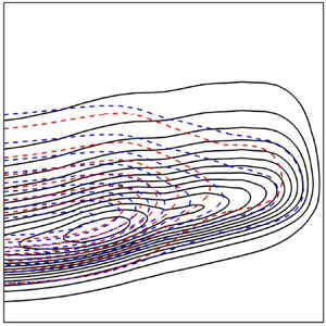
Figure 9. Two-dimensional spectrograms of the inner-normalised premultiplied velocity spectra ($k_x\phi _{uu}/{U_{\tau , p}}^2$) with (i) $U_s = 0$; (ii) $U_s = 1.45\ \textrm {m}\,\textrm {s}^{-1}$; (iii) $U_s = 3.3\ \textrm {m}\,\textrm {s}^{-1}$. The $Re_\tau$ is the lowest in (a) and highest in (e). The vertical dashed line corresponds to $y = k$.

The contours shift upward when $Re_\tau$ increases for all values of $U_s$, revealing the growth of the wavelength $\lambda _x$ of the most energetic turbulent structures with the Reynolds number. Note though that the contours for the two highest $Re_\tau$ (figure 9d,e) are practically the same suggesting that this growth saturate or at least its rate decreases with an increasing Reynolds number. Comparing the cases without and with suction one observes that suction reduces the magnitude of the contours; this effect weakens as $Re_\tau$ increases. This decrease of the spectra amplitude is consistent with the data of figure 3(b). Interestingly, this amplitude reduction reflects not only an increase of $U_{\tau ,p}$ but also an absolute reduction in the energy, as illustrated by figure 4(a) where we already noted that the ratio $\sqrt {\overline {u^2}}/U_1$ in the region $y/k \geq 1$ decreases when suction is applied for all Reynolds numbers. These results show that suction reduces the energy at all scales of motion, in the region above the roughness elements.

While for the shape of the contours are practically unchanged by suction for the two highest $Re_\tau$, they are clearly affected at the other lower $Re_\tau$ (figure 9a–c), particularly for large $\lambda _x$ and $y/\delta$. This is well illustrated in figure 10 where we compare the spectra contours without and with suction for the lowest and largest Reynolds numbers. For the lowest $Re_\tau$, suction narrows the spectra contours in the region $y/\delta > 0.1$. At the highest $Re_\tau$, the contours are barely deformed when suction is applied. These observations may suggest a structural change of the TBL at the lowest Reynolds number when suction is applied. Note that one can expect to observe such structural change at the highest Reynolds number if one increases the suction velocity $U_s$ beyond the current maximum value.

Figure 10. Comparison of contour lines of velocity spectra $(k_x\phi _{uu})/U_\tau ^2$ at three suction velocities ($U_s = 0, 1.45$ and $3.3\ \textrm {m}\,\textrm {s}^{-1}$) for the lowest (a) and highest (b) $Re_\tau$. Contour levels: 0–1.4 in 0.1 increments.

The contour maps (figure 9) for the two largest Reynolds numbers exhibit a behaviour on the lower end of $\lambda _x$ across the boundary layer not observed in the contour maps for the lower Reynolds numbers. The contours indicate that the motions at low $\lambda _x$ become relatively energetic, particularly in the region around $y=k$. At this stage one can speculate on the nature of the physical phenomenon responsible for this ‘extra’ energy. It is possible that the shear layers issued at the roughness elements become energetic enough to leave their imprint on the spectrograms. However, further investigation is required to comment conclusively.

3.5. Comparison with smooth wall

We have argued earlier that the response of the rough wall TBL to suction is different to that of a smooth wall due mainly to the difference in the mechanism for the energy production between the two TBLs. To ascertain this argument, we compare the effect of suction on the distributions of $U$, $\overline {u^2}$ and $S_u$ between the two TBLs at approximately similar $\sigma$ and $Re_\theta$; the smooth wall data are extracted from Oyewola et al. (Reference Oyewola, Djenidi and Antonia2003). Figure 11(a) shows the mean velocity profiles; also shown on that figure are the mean velocity profile for the undisturbed smooth wall TBL and the Blasius profile. When suction is applied on the smooth wall TBL, the distribution $U^+$ follows the Blasius profile up to $y^+ = 30$, revealing the relaminarisation trend impacted by the wall suction on the TBL. This relaminarisation trend reflects the presence of a local favourable pressure gradient induced by the wall suction. Further, as the TBL flows over the suction section, a good part of the inner layer is sucked out, thus disrupting dramatically the production generating process taking place near-the wall and a new inner layer starts to develop downstream of the suction strip. Flow visualisations (Djenidi et al. Reference Djenidi, Gall, Vincent and Antonia2002) showed that downstream of the strip, suction stabilised the near-wall low-speed streaks by reducing their spanwise oscillations while maintaining them closer to the wall for a longer extent as compared with when there was no suction. This indicates that the new inner layer evolves in a laminar-like behaviour which is consistent with the relaminarisation trend shown on the velocity profile. This behaviour is well documented, for example in Antonia et al. (Reference Antonia, Zhu and Sokolov1995), Djenidi & Antonia (Reference Djenidi and Antonia2001), Djenidi et al. (Reference Djenidi, Gall, Vincent and Antonia2002), Oyewola et al. (Reference Oyewola, Djenidi and Antonia2003) and Djenidi, Agrawal & Antonia (Reference Djenidi, Agrawal and Antonia2009). In the case of the rough wall TBL, where the viscous sublayer is practically absent, the turbulence production process is controlled by the roughness elements. Thus, while suction removes part of the inner layer of the incoming TBL, it does not modify the turbulence production mechanism and accordingly does not induce a relaminarisation trend, even though the TBL experiences a local favourable pressure gradient. Further, since the process of turbulence generation is unaffected or weakly affected, one can then expect that the memory effect to be weaker in the rough wall TBL than in the smooth wall TBL which is likely to lead to a shorter length recovery of the former TBL behind the suction strip.

Figure 11. Comparison between the present data $U_s = 0$ ($\diamond$, blue), $U_s = 3.3\ \textrm {m}\,\textrm {s}^{-1}$ (i.e. $\sigma$ = 3.4) ($\diamond$, red) at $Re_\theta = 2050$ and the smooth wall data of Oyewola et al. (Reference Oyewola, Djenidi and Antonia2003) ($Re_\theta$ = 1400, ($\times$) $\sigma = 0$, (${\bigcirc}$) $\sigma = 3.3$). (a) Mean streamwise velocity (dashed line represents the Blasius profile, also extracted from Oyewola et al. (Reference Oyewola, Djenidi and Antonia2003)), (b) turbulence intensity, (c) skewness (dashed line represents the magnitude of skewness in purely Gaussian signal).

Figure 11(b) shows the distribution of ${\overline {u^{2}}}^+$ for both rough and smooth wall TBLs with and without suction; note that the distributions are shown as a function of $y/\delta$. Interestingly, while the mean velocity distribution for the smooth wall TBL with suction indicates relaminarisation, the distribution of ${\overline {u^{2}}}^+$ shows relatively high values of ${\overline {u^{2}}}^+$ in the region around $y/\delta = 0.03$ (or equivalently $y^+ = 13$). Remarkably, the location of the inner local peak of ${\overline {u^{2}}}^+$ in the smooth wall TBL remains unaffected by suction. This is also observed in the laser Doppler measurements of Djenidi et al. (Reference Djenidi, Agrawal and Antonia2009) and the numerical results of Djenidi & Antonia (Reference Djenidi and Antonia2001), but also in the measurements of Fernholz & Warnack (Reference Fernholz and Warnack1998) and Warnack & Fernholz (Reference Warnack and Fernholz1998) in a smooth wall TBL subjected to a favourable pressure gradient. In the case of wall suction, it is likely that the suction rate used was not strong enough to entirely destroy the turbulent energy production mechanism, thus leading to an incomplete relaminarisation. The magnitude of ${\overline {u^{2}}}^+$ in the region $0.1 \leq y/\delta \leq 1$ is reduced by suction. This is in agreement with the presence of a local favourable pressure gradient which has an effect of flattening the distribution of ${\overline {u^{2}}}^+$ in the outer region of the TBL as observed also in Fernholz & Warnack (Reference Fernholz and Warnack1998) and Warnack & Fernholz (Reference Warnack and Fernholz1998). This effect is also felt on the distribution of ${\overline {u^{2}}}^+$ in rough wall TBL when suction is applied.

Finally, we report in figure 11(c) the distributions of $S_u$ for both TBLs with and without suction. In both TBLs, $S_u$ decreases when suction is applied. However, $S_u$ for the smooth wall TBL exhibits a stronger variation, in the form of an oscillation, than its rough wall counterpart within the region $0.07 \leq y/\delta \leq 0.2$. This certainly reflects a stronger structural change in the smooth wall TBL than in the rough wall TBL.

It was noted above that suction may not lead to a complete relaminarisation, which clearly warrants some attention. We thus carried out measurements over a streamwise distance up to $3\delta _0$ (where $\delta _0$ is the initial boundary layer thickness at the leading edge of the suction strip) behind the suction strip. The results are reported in figure 12 which show the streamwise variation of the mean velocity over a vertical distance $0 < y/k < 7$. We used the lowest Reynolds number and highest suction rate since the boundary is most affected under these conditions. As expected, with no suction the velocity presents a periodic behaviour in the streamwise direction, which gradually vanishes as $y/k$ increases. When suction is applied we can also observe the periodic behaviour and its disappearance with increasing $y/k$. However, there is a clear effect of suction. For a fixed $y/k$, the velocity increases. Notice the reverse trend between the no-suction and suction cases. For the former, the general trend is downward, while it is upward in the case of suction. This latter is caused by an inward rush of high-velocity flow caused by a downward flow deflection induced by suction. This trend difference is well captured in figure 13(a,b) which shows isocontours of the streamwise mean velocity. Each figure is almost the symmetric of the other. Figure 13(a) shows a general decrease in the velocity along $x$, while figure 13(b) shows an increase. The downward rush of high-velocity fluid also brings in the low turbulence intensity of the outer region of the flow as seen in figure 14. Interestingly, an increasing level of turbulence is observed (figure 14b) around the roughness elements with increasing $x$, reflecting an increasing turbulence activity in that region of the flow as the boundary layer starts its recovery. These results would confirm that relaminarisation cannot be achieved, or at least cannot be complete, in a rough wall TBL. Consequently, the downstream recovery distance of the TBL should be shorter on a rough wall than on a smooth wall.

Figure 12. Streamwise variation of the mean velocity downstream of suction strip in the region $0.04 < y/\delta < 0.2$ (black lines, $U_s=0$; dashed red lines, $U_s=3.3\ \textrm {m}\,\textrm {s}^{-1}$).

Figure 13. Isocontours of the streamwise mean velocity downstream of suction strip in the region $0.04 < y/\delta < 0.2$ for (a) $U_s=0$ and (b) $U_s=3.3\ \textrm {m}\,\textrm {s}^{-1}$.

Figure 14. Isocontours of the streamwise velocity r.m.s. downstream of suction strip in the region $0.04 < y/\delta < 0.2$ for (a) $U_s=0$ and (b) $U_s=3.3\ \textrm {m}\,\textrm {s}^{-1}$.