


1. Introduction
A fluid exhibits real gas behaviours at thermodynamic conditions above its critical point, known as supercritical conditions. Under the supercritical conditions, the fluid exhibits gas-like transport properties and liquid-like density. Such unique properties make supercritical fluids applicable in various industries, namely: energy, food, biology and pharmaceutical (Givler & Abraham Reference Givler and Abraham1996; Li et al. Reference Li, Zhang, Zhang and Hua2008; Duarte, Mano & Reis Reference Duarte, Mano and Reis2009; Poormahmood, Shahsavari & Farshchi Reference Poormahmood, Shahsavari and Farshchi2018). In some of these applications, turbulent heat, mass and momentum transports play an important role in the process performance. Turbulent mixing has considerable effects on inhomogeneities in the powder particle size produced by the supercritical antisolvent process in pharmaceutical and biopolymer applications (Henczka, Baldyga & Shekunov Reference Henczka, Baldyga and Shekunov2005; Erriguible et al. Reference Erriguible, Laugier, Late and Subra-Paternault2013), methane oxidation rate in supercritical oxidation process of waste (Zhou et al. Reference Zhou, Krishnan, Vogel and Peters2000), supercritical degrading refractory organic wastewater process performance (Zhang et al. Reference Zhang, Su, Chen and Chen2020c), lithium battery nanoparticles production in a supercritical hydrothermal synthesis process (Hong et al. Reference Hong, Kim, Chung, Chun, Lee and Kim2013), supercritical combustion performance and pollutant emissions (Cheng et al. Reference Cheng, Chao, Wu, Hsu and Yuan2001; Mansour et al. Reference Mansour, Elbaz, Roberts, Senosy, Zayed, Juddoo and Masri2017) and film cooling performance under the supercritical conditions (Chang et al. Reference Chang, Du, Zheng, Duan and Liu2019). In this light, controlling the turbulent properties is one of the key ways to tune the process effectiveness under the supercritical conditions.
One of the well known methods to manipulate and control turbulence is to generate coherent motions by triggering hydrodynamic instabilities in the fluid flow field (Mi, Nobes & Nathan Reference Mi, Nobes and Nathan2001). Such methods can be classified into two main groups: passive and active. In the passive group, also known as self-excited methods, the geometry of the device is modified in a way to perturb the flow field (Hasan & Hussain Reference Hasan and Hussain1982) by using wedges (Bradbury & Khadem Reference Bradbury and Khadem1975), piezoelectric actuators (Wiltse & Glezer Reference Wiltse and Glezer1993), vortex-generating tabs (Reeder & Samimy Reference Reeder and Samimy1996; Zaman Reference Zaman1996), microjets and nozzles (Alkislar, Krothapalli & Butler Reference Alkislar, Krothapalli and Butler2007), as well as elliptic (Husain & Hussain Reference Husain and Hussain1983) and rectangular shaped (Tyliszczak & Geurts Reference Tyliszczak and Geurts2015) obstacles. A Gyro-Therm burner is an example of using such passive methods in thermodynamically subcritical combustion devices (Nathan et al. Reference Nathan, Mi, Alwahabi, Newbold and Nobes2006). On the other hand, the active methods use forcing sources experimentally (e.g. varicose (Zaman & Hussain Reference Zaman and Hussain1980, Reference Zaman and Hussain1981; Broze & Hussain Reference Broze and Hussain1994), helical (Koch et al. Reference Koch, Mungal, Reynolds and Powell1989; Corke & Kusek Reference Corke and Kusek1993), flapping acoustic waves (Samimy et al. Reference Samimy, Kim, Kastner, Adamovich and Utkin2007), as well as the mass flow rate excitations (Perumal & Zhou Reference Perumal and Zhou2018) and flexible nozzles (Long & Petersen Reference Long and Petersen1992; Reynolds et al. Reference Reynolds, Parekh, Juvet and Lee2003; Murugappan et al. Reference Murugappan, Gutmark, Lakhamraju and Khosla2008)) or numerically (e.g. varicose (Da Silva & Metais Reference Da Silva and Metais2002; Gohil, Saha & Muralidhar Reference Gohil, Saha and Muralidhar2013), flapping (Gohil & Saha Reference Gohil and Saha2019; Da Silva & Metais Reference Da Silva and Metais2002), dual varicose/helical (Tyliszczak Reference Tyliszczak2015), dual varicose/flapping (Tyliszczak & Geurts Reference Tyliszczak and Geurts2015) perturbations) to stimulate the flow field with tunable frequencies and amplitudes. The active methods have more flexibility to control the instability modes than the passive methods, while the active methods impose extra complexities to the control system. However, triggering the hydrodynamic instabilities may not be always favourable for the process. For instance, flow stimulations can induce oscillations in the combustion field, which may result in thermoacoustic instabilities (Bagheri-Sadeghi, Shahsavari & Farshchi Reference Bagheri-Sadeghi, Shahsavari and Farshchi2013; Shahsavari et al. Reference Shahsavari, Aravind, Chakravarthy and Farshchi2016, Reference Shahsavari, Farshchi, Chakravarthy, Chakraborty, Aravind and Wang2019; Zhang et al. Reference Zhang, Shahsavari, Rao, Yang and Wang2019, Reference Zhang, Shahsavari, Rao, Li, Yang and Wang2020a,Reference Zhang, Shahsavari, Rao, Yang and Wangb). Recently, artificial intelligence methods (Deng et al. Reference Deng, Noack, Morzynski and Pastur2020), deep learning control (Tang et al. Reference Tang, Rabault, Kuhnle, Wang and Wang2020) and optimization techniques (Sau & Mahesh Reference Sau and Mahesh2010; Kim, Bodony & Freund Reference Kim, Bodony and Freund2014; Wu, Wong & Zhou Reference Wu, Wong and Zhou2018; Shaabani-Ardali, Sipp & Lesshafft Reference Shaabani-Ardali, Sipp and Lesshafft2020) have been applied in the flow control to enhance the performance of the control systems.
Utilizing the forcing sources to trigger hydrodynamic instability modes in a supercritical jet can have viable effects on the turbulent flow characteristics. In recent years, various research groups have focused on the effects of varicose perturbations on supercritical/transcritical fluid flows to explore the effects of perturbations on the turbulent mixing and the flow dynamics. Chehroudi & Davis examined effects of plane acoustic waves on supercritical jets (Chehroudi & Talley Reference Chehroudi and Talley2002; Davis & Chehroudi Reference Davis and Chehroudi2007). The results showed that the impact of the acoustic waves on the jets decreases with increasing the chamber pressure. Schmitt et al. studied the effects of longitudinal and transverse varicose perturbations on a coaxial injector operating at supercritical conditions (Schmitt et al. Reference Schmitt, Rodriguez, Leyva and Candel2012). It was shown that the excitations reduce the jets’ potential core length, which is a manifestation of the enhanced turbulent mixing. Hakim et al. studied the effects of transverse varicose mode excitations on a supercritical reacting jet (Hakim et al. Reference Hakim, Schmitt, Ducruix and Candel2015). Results revealed that the flame experiences a flapping motion, when it is excited at the frequency close to the natural frequency of the oxidizer jet. However, the flame is devoid of any bulk motions, when it is modulated at higher frequencies (Hakim et al. Reference Hakim, Schmitt, Ducruix and Candel2015).
The majority of previous investigations considered the effects of varicose mode excitations on supercritical jets. There is still a lack of fundamental knowledge and understanding of the effects of other excitation modes on supercritical jets. To fulfil this gap, a series of large eddy simulations (LES) is performed in the present study to evaluate the roles of a number of different excitation modes (viz. varicose, helical, flapping, dual modes) on supercritical jet characteristics. To achieve such an aim, a correction model is developed to enhance the accuracy of the equation-of-state and transport correlations proposed in the past (Chung et al. Reference Chung, Ajlan, Lee and Starling1988). The present research findings contribute to the design of optimum strategies to manipulate and control turbulent flow properties in various supercritical fluid flow applications aim at increasing the process performance.
2. Numerical method
2.1. Governing equations
The current numerical simulations are performed using a compressible solver developed in the OpenFOAM platform. The present authors have also successfully developed and verified some other solvers in the OpenFOAM platform (Shahsavari, Farshchi & Arabnejad Reference Shahsavari, Farshchi and Arabnejad2017; Shahsavari & Farshchi Reference Shahsavari and Farshchi2018). Turbulence modelling is achieved by using LES. In this solver, a compressible form of the Navier–Stokes equations alongside with the Peng–Robinson (PR) equation-of-state (Schmitt et al. Reference Schmitt, Selle, Ruiz and Cuenot2010) presented as follows are solved via the finite volume method:
 \begin{gather} \frac{\partial \bar{\rho }}{\partial t}+\frac{\partial }{\partial {{x}_{i}}}(\bar{\rho }{{{\tilde{U}}}_{i}})=0, \end{gather}
 \begin{gather}\frac{\partial \bar{\rho }{{{\tilde{U}}}_{j}}}{\partial t}+\frac{\partial }{\partial {{x}_{i}}}(\bar{\rho }{{{\tilde{U}}}_{i}}{{{\tilde{U}}}_{j}})={-}\frac{\partial \bar{P}}{\partial {{x}_{j}}}+({{\bar{\tau }}_{ij}}-\tau _{ij}^{SGS}), \end{gather}
 \begin{gather} \hspace{-3pc}\frac{\partial \bar{\rho }\tilde{h}}{\partial t}+\frac{\partial }{\partial {{x}_{i}}}(\bar{\rho }{{{\tilde{U}}}_{i}}\tilde{h})+\frac{\partial \bar{\rho }\tilde{k}}{\partial t}+\frac{\partial }{\partial {{x}_{i}}}(\bar{\rho }{{{\tilde{U}}}_{i}}\tilde{k})\nonumber\\ \hspace{4pc}= \frac{\partial \bar{P}}{\partial t}+{{\tilde{U}}_{i}}\frac{\partial \bar{P}}{\partial {{x}_{i}}}+\frac{\partial }{\partial {{x}_{i}}}\left( (\alpha +{{\alpha }^{SGS}})\frac{\partial \tilde{h}}{\partial {{x}_{i}}} \right)+\overline{{{\tau }_{ij}}\frac{\partial {{U}_{i}}}{\partial {{x}_{j}}}}, \end{gather}
 \begin{gather} P=\frac{\rho rT}{1-\rho b}-\frac{{{\rho }^{2}}a}{1+2\rho b-{{\rho }^{2}}{{b}^{2}}}, \end{gather}
where,
 \begin{gather} a=0.457236\frac{{{(r{{T}_{c}})}^{2}}}{{{P}_{c}}}{{\left[ 1+( 0.37464+1.54226\omega -0.26992{{\omega }^{2}} )\left( 1-\sqrt{\frac{T}{{{T}_{c}}}} \right) \right]}^{2}}, \end{gather}
 \begin{gather}b=0.077796\frac{r{{T}_{c}}}{{{P}_{c}}}, \end{gather}
and where  $U_{i}$ is the velocity,
  $\rho$ is the density, P is the pressure,
  $\tau _{ij}$ is the stress tensor,
  $\tau _{ij}^{SGS}$ is the subgrid scale stress tensor, h is the enthalpy, k is the kinetic energy,
  $\alpha$ is the thermal diffusivity,
  $\alpha ^{SGS}$ is the subgrid scale thermal diffusivity, T is the temperature, r is
  ${R}/{W}$, R is the perfect-gas constant, W is the molar mass,
  $T_{c}$ is the critical temperature,
  $P_{c}$ is the critical pressure and
  $\omega$ is the acentric factor. The subgrid scale modelling is achieved by using one equation eddy viscosity model (Sagaut Reference Sagaut2001). Moreover,
  $\alpha ^{SGS}$ is calculated by considering the unity turbulent Prandtl number. Here, (
 $\sim$) and (–) denote Favre filtered and filtered quantities, respectively. Chung et al. (Reference Chung, Ajlan, Lee and Starling1988) correlations are adopted in this work to predict the transport properties.
In the present study, a method similar to the volume translation model presented by Abudour et al. is proposed to enhance the accuracy of the PR equation-of-state and Chung et al. (Reference Chung, Ajlan, Lee and Starling1988) correlations in the range of the present chamber operating conditions (Abudour et al. Reference Abudour, Mohammad, Robinson and Gasem2012). In this method, translated variables are calculated by using
 \begin{equation} Va{{r}_{PRC}}=Va{{r}_{PR}}+\frac{R{{T}_{c}}}{{{P}_{c}}}\left( {{b}_{1}}-{{b}_{2}}\exp ({{b}_{3}}d)-\frac{{{b}_{4}}}{{{b}_{5}}+{{b}_{6}}d} \right), \end{equation}
where  $Var_{PRC}$ and
  $Var_{PR}$ are corrected and uncorrected variables (density (
 $\rho$), constant pressure heat capacity (
 $C_{p}$), thermal conductivity (
 $\lambda$)). Moreover,
  $b_{1}$–
 $b_{6}$ are model constants and d is a dimensionless distance function defined as
 \begin{equation} d=\frac{1}{R{{T}_{c}}}{{\left( \frac{\partial {{p}^{PR}}}{\partial \rho } \right)}_{T}}. \end{equation}
 The distance function is calculated from the uncorrected PR equation-of-state. In this study, optimizations are carried out by using Levenberg–Marquardt algorithm (Hansen, Pereyra & Scherer Reference Hansen, Pereyra and Scherer2013) to obtain the model constants by minimizing the absolute percentage deviation (AD) of the predicted variables from the National Institute of Standards and Technology (NIST) database. Moreover, optimizations are also carried on Chung et al. (Reference Chung, Ajlan, Lee and Starling1988) model constants ( $A_{1}$–
 $A_{10}$) to enhance the accuracy of the models. Optimized constants and the improvements of the present models are presented in table 2, which is in the Appendix.
In this study, turbulent filter width is equal to  $(\Delta x\Delta y\Delta z)^{1/3}$. Moreover, the pressure–velocity coupling is achieved using the PIMPLE algorithm, which is a combination of PISO (pressure implicit with splitting of operator) and SIMPLE (semi-implicit method for pressure linked equations) algorithms.
2.2. Numerical discretization
In this study, second-order central difference schemes are used to discretize the convection and diffusion terms. The time derivatives are discretized by a second-order implicit method. The time-step is adjusted to achieve the maximum Courant number of 0.5. All the investigated cases are simulated until they become statistically stationary. Then, numerical data are collected for approximately four flow-through times (i.e. 200 ms) to calculate the average data.
2.3. Computational domain and boundary conditions
Figure 1 shows the present computational domain constructed based on the experimental set-up of Mayer et al. (case 4), in which supercritical nitrogen at a velocity ( $U_z^{inj}$) of
  $5.4 \ \textrm {m}\ \textrm {s}^{-1}$ and a temperature of 137 K is injected through an injector with a diameter (D) of 2.2 mm into a pressurized chamber filled with supercritical nitrogen at 3.97 MPa (Mayer et al. Reference Mayer, Telaar, Branam, Schneider and Hussong2003). The chamber diameter and length are 122 mm and 250 mm, respectively. The Reynolds number based on the injector diameter and the inlet velocity is 160 000. Here, the velocity is fixed at the inlet boundary condition (the injector outlet) by a hyperbolic tangent profile. The ratio of the jet radius to the momentum thickness at the inlet boundary condition is 20. In the present study, randomly distributed spots with root mean square value of 2.5 % of the inlet mean velocity are added to the inlet velocity profiles (Kornev et al. Reference Kornev, Kröger, Turnow and Hassel2007). Moreover, the temperature is fixed at the inlet boundary condition, while a constant pressure is set at the outlet boundary condition. Here, the details of the injector are not included in the simulations, since the experimental data are available at the injector outlet. However, the boundary conditions are set in a way to make sure that the jet experiences no flush motion. A non-reflecting boundary condition is used at the outlet boundary condition. Moreover, a no-slip boundary condition is used on the walls. Constant temperature (298 K) is applied to the chamber walls, except the wall near the injector which is treated as an adiabatic wall.

Figure 1. Sketch of the computational domain and the boundary conditions.
The computational domain is meshed using structured body-fitted grids. The grid size is 0.05 mm near the injector in a cylinder with the diameter and length of 2D and 10D, respectively. This grid size is of the order of the Taylor length scale of the present turbulent flow. The grid is smoothly coarsened toward other sections of the computational domain. The computational mesh contains  $3.5\times 10^{6}$ cells. In order to study the mesh convergence, the numerical simulations are also performed on
  $1\times 10^{6}$ and
  $7\times 10^{6}$ cells.
In this study, the supercritical jet is excited by imposing various perturbation modes on the inlet axial velocity profile using the following forcing function:
 \begin{align} \frac{U_{z}^{f}\left( r,t \right)}{U_{z}^{unf}\left( r,t \right)}&=1+\left\{ {{A}_{v}}\sin (2{\rm \pi} {{f}_{v}}t) \right\} +\left\{ {{A}_{h1}}\sin \left( 2{\rm \pi} {{f}_{h1}}t-{{m}_{1}}\theta \right){{\left( \frac{2r}{D} \right)}^{\left| {{m}_{1}} \right|}} \right\} \nonumber\\ &\quad +\left\{ {{A}_{h2}}\sin \left( 2{\rm \pi} {{f}_{h2}}t+{{m}_{2}}\theta \right){{\left( \frac{2r}{D} \right)}^{\left| {{m}_{2}} \right|}} \right\}, \end{align}
where  $U_{z}^{f}$ is the forced velocity,
  $U_{z}^{unf}$ is the unforced velocity,
  $A_{i}$ (
 ${i}={v},{h}1, {h}2$) are the amplitudes of the excitations,
  $f_{i}$ (
 ${i}={v}, {h}1, {h}2$) are the excitation frequencies, (
 ${r}, \theta$) are the cylindrical coordinates and
  $m_{i}$ (
 ${i}=1, 2$) are the mode numbers. Here, if
  $A_{h1}=A_{h2}=0$ the excitation mode is varicose, if
  $A_{v}=0$ and
  $A_{h1}$ or
  $A_{h2}=0$ the mode is helical, if
  $A_{v}=0$ it is flapping, if
  $A_{h1}$ or
  $A_{h2}=0$ it is varicose/helical dual mode and if
  $A_{v}$ and
  $A_{h1}$ and
  $A_{h2}\ne 0$ the mode is varicose/flapping dual mode. Here,
  $A_{i}$ are considered to be 10 %. Moreover, the mode numbers are set to be 1 for all the investigated cases, since the higher modes rarely happen in real experiments.
The aim of the present study is to compare, for the first time, the effects of various excitation modes on a supercritical jet. For this, the forcing amplitude, Reynolds number and the fluid thermodynamic condition are kept constant. Reynolds et al. (Reference Reynolds, Parekh, Juvet and Lee2003) showed that increasing the flow Reynolds number can diminish the effects of excitations on a subcritical fluid flow. Therefore, a high forcing amplitude should be used to compensate the effects of the high Reynolds number. Further investigations are welcome to study the effects of the forcing amplitude and Reynolds number on linear and nonlinear responses of fluid flows under the external excitations. Moreover, to the best of the present authors’ knowledge, no detailed research has been carried out to address the effects of various excitation modes on subcritical jets. Therefore, further investigations are required to address the effects of thermodynamic conditions on a jet response to the external excitations.
Table 1 summarizes all the numerically investigated cases. Here, ‘V’, ‘H’, ‘F’, ‘VH’ and ‘VF’ stand for varicose, helical, flapping, dual varicose/helical and dual varicose/flapping mode excited cases, respectively. Previous studies showed that exciting subcritical jets with frequencies correspond to the most amplified hydrodynamic instabilities has the highest impacts on the jet features (Crow & Champagne Reference Crow and Champagne1971; Shahsavari & Farshchi Reference Shahsavari and Farshchi2018). In the present study, in order to capture the maximum effects of the excitations on the supercritical jet, the most amplified frequencies in the potential core (1116 Hz) and the transient region (341, 232 Hz) of the unexcited case are used to excite the jet. Moreover, in the dual mode cases,  $f_{h1}$ and
  $f_{h2}$ are chosen in a way to achieve the frequency ratios (
 $f_{v}/f_{h1}$ or
  $f_{v}/f_{h2}$) of 2, 2.5 and 2.25, for which subcritical jets experience considerable bifurcations (Gohil, Saha & Muralidhar Reference Gohil, Saha and Muralidhar2015). In the present study, the most amplified frequencies in the potential core and the transient region are calculated by performing frequency spectrum analyses on the axial velocity fluctuations collected via 120 numerical probes placed at different locations of the potential core and the transient region. Figure 2 presents the energy spectrum of the axial velocity fluctuations at some of the numerical probes. Here, the amplitude of the spectrum in each case is normalized by the corresponding maximum value of the energy spectrum amplitude. Figure 3 plots the azimuthal locations of the dual mode excitation peaks and troughs in the jet cross-section at the inlet boundary condition over time. The angle between the two consecutive peaks or troughs over time is known as the offset angle (
 $\Delta \theta$) (Gohil et al. Reference Gohil, Saha and Muralidhar2015). This angle is related to the forcing frequencies as
  $\Delta \theta =360\times f_{h1}/f_{v}$ in dual varicose/helical mode excitations (Gohil et al. Reference Gohil, Saha and Muralidhar2015). Therefore, the offset angles are
  $180^{\circ }$,
  $144^{\circ }$ and
  $160^{\circ }$ in VH1, VH2 and VH3 cases, respectively. However, the offset angle is
  $180^{\circ }$ in the dual varicose/flapping mode excited cases, when
  $f_{h1}=f_{h2}$. Figure 3 shows that the jet splits into two branches under VH1, VF1, VF2 and VF3 excitation modes, while it experiences five and nine local maxima during VH2 and VH3 excitation modes, respectively.

Figure 2. Energy spectrum of the axial velocity fluctuations in the potential core ( ${Z/D}=3$) and the transient region (
 ${Z/D}=9$ and 12).

Figure 3. Azimuthal locations of the excitation peaks and troughs for the frequency ratios of (a) 2, (b) 2.5 (c) 2.25 over time.
Table 1. Investigated cases.

3. Verification and validation
3.1. Grid independency and validations
There are numerous valuable experimental investigations on supercritical fluid flows in the literature (Oschwald & Schlik Reference Oschwald and Schlik1999; Chehroudi et al. Reference Chehroudi, Cohn, Talley and Badakhshan2000; Chehroudi, Talley & Coy Reference Chehroudi, Talley and Coy2002; O'Neill, Soria & Honnery Reference O'Neill, Soria and Honnery2004; Chehroudi Reference Chehroudi2012). However, in the majority of such cases, the density drops considerably in the supercritical jet, as soon as the jet exits the injector. Banuti & Hannemann showed that the absence of the dense potential core in such cases is due to the thermal breakup mechanism, which initiates inside the injector due to a considerable amount of heat, transferred from the injector walls to the fluid flow (Banuti & Hannemann Reference Banuti and Hannemann2016). Details of such heat transfer are not available in the majority of the experimental cases in the literature, except for the Mayer et al. cases (Mayer et al. Reference Mayer, Telaar, Branam, Schneider and Hussong2003). Therefore, Mayer et al. cases are chosen to validate the current solver. Moreover, Mayer et al. case 4 is selected to study the effects of various excitation modes on a supercritical jet in the following sections of the present work. In order to further validate the current numerical solver, numerical simulations are carried out to reproduce Xu & Antonia's experimental data on a subcritical round jet (Xu & Antonia Reference Xu and Antonia2002), and direct numerical simulation results obtained by Gohil et al. on a subcritical round jet excited with dual varicose/helical mode perturbations (Gohil et al. Reference Gohil, Saha and Muralidhar2015).
Figure 4(a) plots time-averaged density distributions along the combustor centreline obtained from the present numerical simulations as well as the experimental data presented by Mayer et al. (cases 3 and 4). Details of the computational domain, the momentum thickness, the boundary conditions and the inlet turbulent intensity in Mayer et al. case 3 are similar to the corresponding details used to simulate case 4, as presented in § 2.3. Moreover, the utilized grid topology in case 3 is similar to the finest grid used to perform the simulations in case 4. The simulations are performed to get the statistically stationary data. Then, the numerical results are collected for approximately four flow-through times to calculate the averaged data. In case 3, a transcritical jet at a velocity of  $4.9\ \textrm {m}\ \textrm {s}^{-1}$ (
 ${Re}=170\,000$) and a temperature of 126.9 K is injected into the pressurized chamber at 3.97 MPa. In addition, the numerical result obtained from LES by Schmitt et al. for case 4 is also included in figure 4(a) (‘Schmitt2010(LES)-Case4’) (Schmitt et al. Reference Schmitt, Rodriguez, Leyva and Candel2012). The results show that the intermediate (figure 4a, ‘Present_ModifiedPR-Case4(3.5M)’) and fine meshes (figure 4a, ‘Present_ModifiedPR-Case4(7M)’) used to simulate case 4, correctly predict the potential core breakdown distance, where the density starts dropping dramatically. However, at the downstream regions of case 4, the coarse grid (figure 4a, ‘Present_ModifiedPR-Case4(1M)’) has lower discrepancies with the experimental data than the other meshes. However, the intermediate mesh was chosen in the present study to achieve the grid independent results with the minimum computational expenses. Here, additional numerical simulations are also performed on case 4 using the original PR equation-of-state and Chung et al. correlations on the medium mesh (figure 4a, ‘Present_OriginalPR-Case4(3.5M)’) to assess the effects of the proposed modifications on the overall features of the supercritical jet. Figure 4(a) shows that the original models predict a shorter potential core than the modified models. Moreover, as it is expected, the original models overpredict the potential core density. However, the modifications have negligible effects on the mean density distribution downstream of the potential core breakdown location. Figure 4(a) also shows that the numerical simulation using the original PR equation-of-state well reproduces the experimental data on case 3. The results of case 4 reveal that, similar to the Schmitt et al. (Reference Schmitt, Selle, Ruiz and Cuenot2010) data, the present numerical simulations have discrepancies with the experimental data at
  $Z/D>6$. The discrepancies may be due to the experimental errors introduced by Mayer et al. (Reference Mayer, Telaar, Branam, Schneider and Hussong2003) including plasma formation and loss of the laser energy due to high refraction index gradient, linear assumption between density and Raman signal, and a limited number of statistics (56 images) used to obtain the averaged results. Moreover, Banuti showed that the discrepancies can be due to the adiabatic assumption utilized in the injector wall in the numerical simulations (Banuti & Hannemann Reference Banuti and Hannemann2016). Another manifestation of the above-mentioned sources of errors is the non-constant density distribution in the potential core of cases 3 and 4 (
 $Z/D<5$) as shown in figure 4(a). Moreover, based on the NIST database, nitrogen density at
  $T=137\ \textrm {K}$ and
  $p=3.97\ \textrm {MPa}$ is
  $163.5 \ \textrm {kg}\ \textrm {m}^{-3}$. However, the mean experimental value of the density in the potential core (
 $Z/D<5$) is approximately
  $165\ \textrm {kg}\ \textrm {m}^{-3}$ in case 4, which indicates that the inlet temperature or pressure might be slightly lower than the reported values in case 4.

Figure 4. (a) Time-averaged density distribution along the non-dimensionalized axial direction in supercritical and transcritical round jets, (b) radial distributions of non-dimensionalized time-averaged axial velocity and Reynolds shear stress in a subcritical round jet at  $Z/D=3$ and 20, (c) radial distributions of the non-dimensionalized time-averaged axial velocity in a subcritical round jet under dual varicose/helical excitations at
  $Z/D=3$, 4, 5, 6.5 and 8.
The Xu & Antonia case comprises of a turbulent, round subcritical jet injected through a conventional contraction jet with the Reynolds number of 86000, calculated based on the injector exit: diameter (D) and velocity (Xu & Antonia Reference Xu and Antonia2002). The computational domain utilized in this case comprises of a cylinder with 25D and 40D diameter and length, respectively. The domain is meshed with  $6.7\times 10^{6}$ cells using the same mesh topology as the one utilized in the present study to simulate Mayer et al. case 4. A non-reflecting boundary condition is used at the outlet. Moreover, a no-slip boundary condition is used on the walls. The operating pressure is set to be 101 325 Pa. The numerical simulations are performed to get the statistically stationary data. Then, the results are collected for approximately four flow-through times to obtain the averaged data. The simulations are carried out for the Xu & Antonia case by using the experimentally measured exit mean velocity profile of the injector alongside with 0.5 % initial turbulent velocity. Figure 4(b) plots the radial distributions of the mean axial velocity and the Reynolds shear stress at
  $Z/D=3$ and 20 obtained from the present numerical simulations and the experimental investigations performed by Xu & Antonia (Reference Xu and Antonia2002). Here,
  $U_{c}$ is the axial velocity at the jet centre at each axial location. The results show that the present numerical solver can reproduce both the mean and Reynolds stress details of the experimental data in both near (
 $Z/D=3$) and far (
 $Z/D=20$) field regions of the turbulent round subcritical jet.
The main objective of the present paper is to evaluate the effects of various excitation modes on a supercritical jet. Therefore, it is mandatory to examine the capability of the present numerical solver in predicting round jet details under the external excitations. To achieve this, numerical simulations are performed on a round jet at  $Re=2000$ (calculated based on the injector exit: diameter (D) and velocity (
 $U_z^{inj}$)) excited with dual varicose/helical mode excitations, which was simulated by Gohil et al. using direct numerical simulations (Gohil et al. Reference Gohil, Saha and Muralidhar2015). The computational domain comprises of a cylinder with 25D and 15D diameter and length, respectively. The domain is meshed with
  $5.1\times 10^{6}$ cells using the same mesh topology as the one utilized in the present study to simulate Mayer et al. case 4. A non-reflecting boundary condition is used at the outlet, while a no-slip boundary condition is used on the walls. The operating pressure is set to be 101 325 Pa. The simulations are carried out to get the statistically stationary data. Then, the numerical results are collected for approximately four flow-through times to calculate the averaged results. In this case, the ratio of the jet radius to the momentum thickness at the inlet boundary condition is 20, the ratio of varicose-to-helical forcing frequencies is 2, and
  $St_{v}=0.5$ and
  $A_{h1}=A_{v}=5\,\%$ (Gohil et al. Reference Gohil, Saha and Muralidhar2015). Figure 4(c) compares the present numerical results with Gohil et al. DNS data on the bifurcating plane. The results show the present solver can predict details of round jets under the external excitations. The excited jets show a single hump feature at
  $Z/D=4\text {--}5$, while at farther downstream distances (
 $Z/D=6.5$ and 8), the jet splits into two arms due to the bifurcation.
3.2. Further analyses of the unexcited jet
Figure 5 shows the density distribution of the unexcited supercritical jet. Note that the term ‘unexcited jet’ means the uncontrolled excited jet, since there is no disturbance-free turbulent flow in nature (Hussain Reference Hussain1981). In other words, the unexcited jet is not stimulated by any controlled excitations. However, it experiences various natural instabilities. Here, isolines of the zero axial velocity are used to discern vortices. Moreover, streamlines are shown for a portion of the shear layer in the embedded subfigure. The results show that vortices are generated on the lighter fluid side of the shear layer formed between the jet and the chamber flow field due to Kelvin–Helmholtz instabilities. Such vortices induce wavy structures on the supercritical jet (density profile) near the injector. They evolve into vortex-like structures farther downstream of the injector. In figure 5, CV and CVL show the centre of vortices and vortex-like structures, respectively. The result shows that the centre of vortices (e.g. CV1 shown in the embedded graph in figure 5) and the centre of the vortex-like structures on the supercritical jet (e.g. CVL1 shown in the embedded graph in figure 5) do not overlay each other. Moreover, the vortex-like structures on the supercritical jet are not always accompanied by vortices (e.g. CVL2 shown in figure 5). Therefore, it is clear that the turbulent structures (vortices) are affected strongly by some stabilization mechanisms. One of these stabilization mechanisms is the steep density gradient induced by the stratified supercritical shear layer (Zong et al. Reference Zong, Meng, Hsieh and Yang2004; Bellan Reference Bellan2006). The steep density gradient induces dissipation near the high-density gradient region (Bellan Reference Bellan2006), which dampens turbulent fluctuations in the direction perpendicular to the jet, while it increases the fluctuations in the direction horizontal to the jet (Zong et al. Reference Zong, Meng, Hsieh and Yang2004; Bellan Reference Bellan2006; Lapenna & Creta Reference Lapenna and Creta2019). Flow stratification can also reduce the fluid entrainment into the vortices and the frequency of vortex pairing and turbulence intensity (Atsavapranee & Gharib Reference Atsavapranee and Gharib1997). Similar to the subcritical stratified shear layers, the negative turbulence production on the heavy side of the variable-density jet might act as another stabilization mechanism. The negative turbulence production can be due to the negligible axial gradient stretching and turbulent mass flux on the heavier side of the stratified shear layer (Charonko & Prestridge Reference Charonko and Prestridge2017).

Figure 5. Instantaneous density distribution alongside with isolines of the zero-axial velocity and streamlines of the unexcited supercritical jet.
In order to further identify the stratified supercritical shear layer properties, here numerical analyses are carried out on the vorticity equation source terms. Figure 6 compares vorticity budgets and the locations of the velocity and density profiles’ inflection points at different axial locations of the jet. The mean value of all budget terms (figure 6, ‘Mean’) and the mean density profile (figure 6, ‘ $\langle \rho \rangle$’) are shown for the reference.

Figure 6. Radial distribution of the time-averaged vorticity budgets and density at various cross-sections of the unexcited supercritical jet; (a)  $Z/D=0.5$, (b)
  $Z/D=1.5$, (c)
  $Z/D=2.5$.
It can be seen from figure 6 that the density and velocity inflection points overlay each other near the injector ( $Z/D=0.5$). Therefore, this location corresponds to a region in which Kelvin–Helmholtz instabilities are amplified (Raynal et al. Reference Raynal, Harion, FavreMarinet and Binder1996). Intense mean vorticity sources, mainly induced by viscosity, dilatation and baroclinic, near the inflection points at
  ${Z/D}=0.5$ as compared with other locations, are a manifestation of the disturbance amplifications. However, as the jet moves downstream, the density and velocity inflection points move apart from each other and the mean value of the vorticity budget decreases. Density and velocity inflection points move toward the heavier and lighter fluid sides of the shear layer, respectively. The results reveal that there are vorticity sinks at the boundary of the shear layer, near the injection point. The strength of the vorticity sinks on the lighter fluid side is higher than the heavier fluid side of the shear layer. However, the vorticity sinks disappear as the jet moves downstream. In the vicinity of the injector (
 $Z/D=0.5$), baroclinic, viscosity and dilatation are the key vorticity sink terms on the lighter fluid side, while on the heavier fluid side of the shear layer, the viscosity term is the only sink. At farther downstream locations (
 $Z/D=1.5$), dilatation is also a vorticity sink in both sides of the shear layer. As the jet moves downstream (
 $Z/D=2.5$), the vorticity sink strength drops on both sides of the shear layer. At such locations, baroclinic is almost the only term that acts as a vorticity sink in the shear layer. Based on the above-mentioned results and observations, the shear layer experiences high vorticity sinks, where the shear layer is devoid of any large wavy structure near the injector (see figure 5). However, the vorticity sinks lose strength at the downstream regions, where the wavy structures grow in size.
In order to evaluate the supercritical jet dynamics, frequency spectrum analyses are carried out on the axial velocity fluctuations along the jet centreline to obtain amplified frequencies of the flow at different locations (120 probes) of the supercritical jet; the potential core and the transition region. In the present supercritical jet, the potential core length is 4.3D, which is measured by tracking the location, where the centreline density drops to 99 % of the inlet jet density. This length is in the range of the potential core length of an incompressible turbulent jet, which is approximately 3–5 times the burner diameter (Ho & Huerre Reference Ho and Huerre1984). It should be mentioned that Mayer et al. showed that the flow does not reach a self-similar condition at  $Z/D<20$. Similar analyses carried out in the present study (not presented here) show that the supercritical jet does not reach self-similar conditions at
  $Z/D<50$. However, the main objective of the present study is to evaluate the effects of various excitation modes on the supercritical jet. As is shown in the following sections, the excitations decay dramatically at
  $Z/D>15$. Therefore, investigating the flow characteristics at
  $Z/D>50$ is beyond the scope of the present study.
The frequency spectrum analyses show that the supercritical jet experiences high-frequency (2278 Hz) low-amplitude perturbations, which is the initial shear layer instability mode detected here, at the vicinity of the inlet. The present studies show that the frequency of the most amplified mode of the hydrodynamic instabilities in the potential core (preferred mode) is 1116 Hz, which approximately equals the second subharmonic of the initial instability frequency. In subcritical mixing layers, the preferred mode frequency, the most amplified frequency in the potential core, is in the second to third subharmonic range of the initial shear layer instability frequency (Schadow & Gutmark Reference Schadow and Gutmark1992). Therefore, the ratio of the preferred mode frequency to the initial instability frequency in the present supercritical jet is of the order of the corresponding ratio in subcritical jets. Previous investigations showed that the preferred mode Strouhal numbers ( ${St}={f\kern0.05em D}/U_z^{inj}$, where f is frequency and
  $U_z^{inj}$ is the jet injection velocity) of subcritical shear layers are in the range of 0.25–0.5 (Gutmark & Ho Reference Gutmark and Ho1983). Here, the preferred mode Strouhal number is 0.45, which is in the range of the Strouhal numbers of the preferred modes of the subcritical fluid shear layers. It is well known that the amplified hydrodynamic frequency of jets decreases in the farther downstream regions of the potential core due to turbulent mixing. In the present supercritical jet, the amplified frequency at each axial location fits with
  $4838(Z/D)^{-1.235}$. Obtained results show that the most amplified frequencies in the transient region of the present supercritical jet are 232 and 341 Hz at
  $4.3 < Z/D < 10$ and
  $10 < Z/D < 20$, respectively.
Similar frequency spectrum analyses on the axial velocity fluctuations are carried out on the numerical simulation results utilized the original PR equation-of-state and Chung et al. (Reference Chung, Ajlan, Lee and Starling1988) correlations to evaluate the effects of the proposed modifications on the jet dynamics. It is found that the most amplified mode frequencies in the potential core and the transient regions are 1067 and 358 Hz, respectively. Therefore, the proposed modifications result in changes in the most amplified mode frequencies by 4 %–5 %.
4. Results and discussion
The present section is concerned with the effects of different excitation modes on the supercritical round jet features including: (i) coherent structures; (ii) jet development; and (iii) turbulent kinetic energy.
4.1. Coherent structures
Coherent structures are believed to strongly affect turbulent mixing, hydrodynamic features, flow noise and various hydrodynamic and thermoacoustic instabilities (Fiedler Reference Fiedler1988; Zhang et al. Reference Zhang, Shahsavari, Rao, Yang and Wang2019, Reference Zhang, Shahsavari, Rao, Li, Yang and Wang2020a). Changing the coherent structure features can manipulate turbulent flow characteristics, which has great technical relevance. Enhancement and manipulation of coherent structures are possible by imposing periodic excitations on the jet (Ho & Huerre Reference Ho and Huerre1984). Moreover, it is of both practical and fundamental interest to study coherent structure features, when the jet experiences hydrodynamic instabilities. In the present paper, the supercritical jet is excited by various forcing waves to address both of the above objectives; manipulating coherent structures by periodic excitations and features of coherent structure in a hydrodynamically unstable jet.
This section discusses the effects of the imposed excitations on various aspects of the coherent structures in the investigated supercritical jets. To sum up the aims, the Q-criterion is used to educe the coherent structures, which are illustrated in figure 7 for the investigated cases. All coherent structures are shown at the value of 3 % of the maximum value of Q in each case for all the following analyses. In figure 7, the structures are coloured by the root mean square of density fluctuations to show the contribution of coherent motions in inducing density fluctuations and turbulent mixing. The results show that a multitude of coherent structure forms including helix, ring, line or rib, and hairpin appear in the supercritical jets. Similar to the most axisymmetric jets, coherent structures are single-helix-like near the injector for all the investigated cases. The single-helix structures are the first mode of the vortical structures in axisymmetric jets (Fiedler Reference Fiedler1988). However, the structures evolve into ring-like structures farther downstream of the injector due to the varicose perturbations in V1, VH1, VH2, VH3, VF1, VF2 and VF3 cases. Although V2 and V3 cases are also stimulated by the varicose perturbations, they are devoid of any ring-like structures. This is in line with the results presented in the previous sections, in which it is found that the varicose excitations have limited effect on the supercritical jet, when the forcing frequency matches the most amplified frequencies in the transient region. Figure 7 also shows that some sort of ring-like structures tilted toward the radial direction are also observed in the supercritical jet excited by flapping mode perturbations. It is interesting to note that the structures show similar features near the injector in the dual mode excited cases in comparison with the case V1. Therefore, the varicose part of the dual mode excitations has the dominant effect on the coherent structures in the potential core. The present results also show that line (or rib) and hairpin coherent structures appear between the ring-like structures in case V1 and dual mode excited cases. Such structures are generated during the formation of the ring-like elements from the helix structures. Farther downstream of the above-mentioned highly organized structures, a complex agglomeration of coherent structures observed in the flow field, which are produced from the cut-and-connect mechanism (Hussain Reference Hussain1986). This mechanism comprises of breakdowns, interactions and interconnections of the organized coherent structures. Such complex topology of the vortex filaments becomes irregular as the flow moves downstream. In all tested cases, the coherent structures induce negligible density perturbations in the potential core, while as the potential core breaks down, they induce huge density perturbations. Farther downstream, the density perturbations through the coherent structures are decreased significantly.

Figure 7. Coherent structures shown by Q-criterion (@ 3 % of  $Q_{Max}$) coloured by the root mean square density fluctuations.
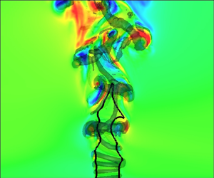
Figure 7 also reveals that VH1, VH2, VH3, VF1, VF2 and VF3 cases experience bifurcations at downstream regions of the injector, through which structures are shed toward different branches, which are shown by solid lines. This is consistent with the bifurcations reported in subcritical jets (Danaila & Boersma Reference Danaila and Boersma2000; Gohil et al. Reference Gohil, Saha and Muralidhar2015; Tyliszczak Reference Tyliszczak2015). Previous investigations show that the bifurcation in dual varicose–helical mode excited subcritical jets is the result of self-induced velocity normal to a vortex ring induced by the tilting of the vortex due to the uneven distribution of vorticity and convective velocity inside the vortex ring (Gohil et al. Reference Gohil, Saha and Muralidhar2015). Such uneven distributions are due to the helical perturbations (Gohil et al. Reference Gohil, Saha and Muralidhar2015). Details of the bifurcation phenomenon in the present supercritical jet are illustrated in figure 8, which plots the spatial distribution of the instantaneous tangential velocity alongside with the isosurface of Q criterion and the isoline of density. Here, the isosurface of the density at 99 % of the maximum value of density is used to show the jet potential core. It can be seen in the zoomed-in graph in figure 8 that the self-induced velocity normal to the vortex ring (tangential velocity) is already present upstream of the potential core breakdown and the bifurcation location. Therefore, although the self-induced velocity is the necessary criterion to induce bifurcation in the dual mode excited cases, it is not sufficient. Results show that the self-induced velocity results in bifurcation downstream of the potential core, where the stratified shear layer stabilization mechanisms decay significantly. Therefore, the bifurcation takes place, if the self-induced velocity overthrows the stabilization mechanisms, which necessarily takes place downstream of the potential core.

Figure 8. Spatial distribution of the instantaneous azimuthal velocity alongside with isosurface of  $0.03Q_{Max}$ criterion and isoline of
  $0.99\rho _{Max}$ in case VF1.
As it is shown in figure 3, the supercritical jet experiences the highest amplitude perturbations at two distinct azimuthal locations in VH1, VF1–VF3 cases, while in VH2 and VH3 cases, five and nine distinct locations in the azimuthal direction experience the highest amplitude perturbations, respectively. Although the twofold coherent structure shedding is clearly observed in figure 7 for VH1, VF1–VF3 cases, the fivefold and ninefold patterns are rarely observed in VH2 and VH3 cases. In order to further shed light onto the bifurcations in the dual mode excited cases, figure 9 shows isolines of the time-averaged axial velocity at the values of 0.5 and  $2\ \textrm {m}\ \textrm {s}^{-1}$ along with isosurfaces of the axial velocity at the value of
  $2 \ \textrm {m}\ \textrm {s}^{-1}$ coloured by the time-averaged density. The results show that the circular jet cross-section at
  $Z/D<5$ evolves into a more elliptic shape as the supercritical jets in VH1, VF1–VF3 cases move into the downstream regions (
 $Z/D>5$). Among these numerically tested cases, just VH1 and VF1 cases experience twofold patterns at
  $Z/D>10$. The results show that the jet cross-section is almost circular at different axial locations in VH2 and VH3 cases. Therefore, the high modes of the bifurcation (fivefold and ninefold cases, VH2 and VH3) are hardly trackable in the averaged results under the supercritical condition. Reynolds et al. showed that the existence of the multiarm patterns in subcritical fluid flows is highly dependent on the flow Reynolds number (Reynolds et al. Reference Reynolds, Parekh, Juvet and Lee2003). The multiarm patterns are well produced at low Reynolds numbers (e.g. 2000–3000) (Gohil et al. Reference Gohil, Saha and Muralidhar2015; Tyliszczak Reference Tyliszczak2015). However, the present study shows that the averaged flow field is devoid of the multiarm patterns at high Reynolds number supercritical fluid flows, due to the high level of turbulent mixing under the high-Reynolds-number condition. The density distribution on the isosurfaces of the axial velocity shows that the density field does not follow exactly the same multifold patterns as the velocity field. For instance, in the cases of VH1 and VF1, the fluid density is at the maximum value at the central part of the jet at
  $Z/D>5$.

Figure 9. Isolines of the time-averaged axial velocity (at 0.5 and  $2\ \textrm {m}\ \textrm {s}^{-1}$) along with the isosurface of the axial velocity at
  $2\ \textrm {m}\ \textrm {s}^{-1}$ coloured by the time-averaged density.
In order to further analyse the coherent structure features under the imposed excitations, figure 10 presents the pitch distance between the coherent structures in the axial direction averaged over the snapshots of the simulations ( $\langle L_{P}\rangle$). The pitch distance (as shown in the embedded graph in figure 10) is an axial distance between the crest of structures at Z–r planes. Here, just helix and ring structures are considered to measure the pitch distance. Both the axial coordinate and the pitch distance are normalized by the injector diameter. In the dual mode excited cases, only coherent structures before the bifurcations are considered here. Figure 10 shows that unexcited, V2, V3 and helical cases have a similar pitch distance pattern in the axial direction. In such cases, the pitch distance increases linearly with the axial direction. However, in the other numerically tested cases (V1 and dual modes), the pitch distance grows in the axial direction in a logistic pattern (increases exponentially at low Z/D, while it levels off at the downstream regions). Here, the distance between the injector outlet and the axial location, where the last coherent helix or ring structures are observed, is defined as the coherent structure penetration depth (
 $\langle L_{CS}\rangle$). The normalized values of the penetration depth are given in the legend of figure 10. Obtained results show that coherent structures in case F have the least penetration depth, while they have the maximum penetration depth in case V1 among the investigated cases. The results show that the coherent structures have more penetration depth in the dual varicose/helical excited cases as compared with the dual varicose/flapping excited cases.

Figure 10. Non-dimensionalized coherent structure pitch distance along the non-dimensionalized axial direction.
Coherent structures are not necessarily highly energetic in turbulent flows. The level of the energy through the coherent structures is dependent upon the flow regime. In fully developed flows, the turbulent energy through coherent structures is comparable with incoherent turbulent motions, while in transitional flows, they contain the majority of the turbulent energy (Hussain Reference Hussain1986). The question posed here concerns the key effects of the excitations on the turbulent energy level though the coherent structures in the present supercritical jet. This energy can be monitored by evaluating the fraction of the total turbulent kinetic energy attributed to the coherent structures ( $k_{CS}(\%)=100\times E_{CS}/E$, where E and
  $E_{CS}$ are the total kinetic energy and the corresponding energy through the coherent structures, respectively). The previous investigations show that
  $k_{CS}$ is approximately 20 % in plane mixing layers, 25 % in accelerated mixing layers, 50 % in near jets, 10 % in axisymmetric far-jets, 25 % in near wakes and 20 % in plane far-wakes (Fiedler Reference Fiedler1988). In order to calculate
  $k_{CS}$ in the present supercritical jets, a cylindrical subdomain of the computational domain near the injector with the length and diameter of 10D and 5D, respectively, is chosen to calculate both the total turbulent kinetic energy and the corresponding value through the coherent structures. Here, the coherent structures are discerned via the Q-criterion at the value of 3 % of the maximum value of Q in each case. Then, the kinetic energy through the coherent structures (
 $E_{CS}$) is integrated in the marked volume using the Q-criterion. Moreover, the total value of the kinetic energy (E) is calculated by integrating the kinetic energy through the subdomain near the injector. Then, the averaged value of
  $k_{CS}$ is measured using the snapshots of the numerical simulations. The present obtained results show that this ratio is 15.6 % in the unexcited jet. In order to compare
  $\langle k_{CS}\rangle$ in different cases appropriately,
  $\langle k_{CS}\rangle$ in the excited cases are normalized by the corresponding value in the unexcited jet. Figure 11 compares the normalized value of the fraction of the kinetic energy attributed with the coherent structures in the investigated cases. It is interesting to note that
  $\langle k_{CS}\rangle$ drops considerably in the excited cases as compared with the unexcited case. More specifically, the fraction of the turbulent kinetic energy through the coherent structures in V1 and dual mode excited cases is less than 80 % of
  $\langle k_{CS}\rangle$ in the excited case. This is consistent with the previously observed turbulence suppression near the exit of an axisymmetric jet under external excitations (Zaman & Hussain Reference Zaman and Hussain1981). Figure 7 shows that the coherent structures are more coherent and larger in V1 and dual mode excited cases as compared with the corresponding structures in the other cases. It can be concluded that the coherent structures carry less turbulent energy, if the imposed excitations create large scale coherent structures. As it is observed from the cases of V2, V3, H and F, figure 7, structures are smaller than the structures observed in V1 and the dual mode excited cases. Therefore,
  $\langle k_{CS}\rangle$ is higher in V2, V3, H and F cases as compared with V1 and the dual mode excited cases.

Figure 11. Normalized kinetic energy and helicity through the coherent structures.
Helicity is one of the key features showing connections between coherent structures and the supercritical turbulent flow. This variable measures the orthogonality of the coherent structures or vortices with the local velocity (Moffatt Reference Moffatt1969). If the coherent structures are orthogonal to the local velocity, the helicity is zero. This means that the structures have two-dimensional motions in nature. On the other hand, the non-zero helicity indicates that the structures have three-dimensional motions. Here, helicity is integrated over the coherent structures in each case using a similar methodology as the one used to measure  $\langle k_{CS}\rangle$. Next, the helicity in each excited case is normalized by the corresponding value of the unexcited jet. Figure 11 shows that the helicity drops in all excited cases as compared with the unexcited case.
The results clearly reveal that the degree of three-dimensionality of the coherent structures reduces when the supercritical jet stimulated by any kind of harmonic perturbations. Such effects are at the maximum value in V1 and the dual mode excited cases. Among the numerically tested cases, the dual varicose/flapping mode excitations with the frequency ratio of 2 have the maximum effect on the helicity. However, the varicose mode excitations with the frequency matching the most amplified frequency in the transient region (V2 and V3 cases) as well as the helical and the flapping mode excitations have the least effect on the local helicity.
4.2. Jet development
Characterizing the effect of the excitations on the flow development region is achieved by comparing the potential core length in the unexcited and excited cases. This is shown in figure 12. The potential core length is measured based upon both density and velocity profiles,  $L_{\langle \rho \rangle }$ and
  $L_{\langle Uz\rangle }$, respectively, which are normalized by the injector diameter (D). The end of the potential core is measured by tracking the location, where the centreline density (or velocity) profile drops to 99 % of the corresponding variables at the inlet.

Figure 12. Non-dimensionalized potential core length based upon density and velocity profiles.
Figure 12 reveals that, unlike the unexcited and excited cases under the varicose excitations (V1–V3 cases), in cases under the helical (case H), the flapping (case F) and the dual mode (VH1–VH3 and VF1–VF3 cases) excitations, the potential core length calculated based on the density profile is considerably shorter than the potential core length measured based on the axial velocity profiles. The results show that the length of the flow development region drops drastically under the flapping (case F) and the dual mode excitations (VH1–VH3 and VF1–VF3 cases), while the varicose excitations with the frequency matching the most amplified frequencies in the transient region (V2 and V3 cases) have negligible effect on the potential core length.
The effects of the imposed excitations on the supercritical jet are further studied by evaluating the pseudo-similarity behaviours of the supercritical jet under both unexcited and excited conditions. The aim is to search for a similarity between the unexcited and excited supercritical jets as well as subcritical constant and variable density jets. To such an aim, non-dimensional density and axial velocity are plotted in figure 13 along the jet axis in search for pseudo-similarity. Here, the density and the axial velocity are normalized as
 \begin{gather} {u}^{*}=\frac{\langle U_{z}^{inj}\rangle }{\langle {{U}_{z}}\rangle}, \end{gather}
 \begin{gather}{{\rho }^{*}}=\frac{\langle {{\rho }^{inj}} \rangle -\langle {{\rho }^{\infty }} \rangle }{\langle \rho \rangle -\langle {{\rho }^{\infty }} \rangle }, \end{gather}
where,  $\langle {\rho }^{\infty } \rangle$ is the time-averaged far field density,
  $\langle U_{z}^{inj} \rangle$ and
  $\langle {\rho }^{inj} \rangle$ are the time-averaged axial velocity and density at the inlet, respectively. Variable-density jets show no similarity when the coordinate is normalized by the injector diameter (Schmitt et al. Reference Schmitt, Selle, Ruiz and Cuenot2010). In this light, the coordinate is usually normalized by an effective diameter (
 $d_{\alpha }^{eff}$ ), which is defined as
 \begin{equation} d_{\alpha }^{eff}=D{{\left( \frac{\langle {{\rho }^{\infty }} \rangle }{\langle {{\rho }^{inj}} \rangle } \right)}^{\alpha }}, \end{equation}
where,  $\alpha$ is a constant. Here,
  $\alpha$ is set to be
  $-1/2$ and 1/2 to plot the normalized velocity and density profiles, respectively. Moreover, the potential core length is subtracted from the axial coordinate to ignore the negligible changes of the axial velocity and the density in the potential core. Some of the previous analyses carried out on the low-pressure constant density (Chassaing_1) and variable density with
  ${\rho }^{inj}$/
 ${\rho }^{\infty }=1.43$ (Chassaing_1.43) jets as well as a high-pressure jet with
  ${\rho }^{inj}$/
 ${\rho }^{\infty }=7.9$ (Zong_7.9) are also presented in figure 13 for reference (Chassaing Reference Chassaing1979; Zong Reference Zong2005). It is worth noting that
  ${\rho }^{inj}$/
 ${\rho }^{\infty }$ is 3.6 for the present supercritical jets, where
  ${\rho }^{inj}$ is the fluid density at the injector outlet and
  ${\rho }^{\infty }$ is the far-field fluid flow density.

Figure 13. Normalized (a) velocity and (b) density distributions along the normalized axial direction. The potential core lengths based upon the velocity and density profiles ( $L_{\langle Uz\rangle }$ and
  $L_{\langle \rho \rangle }$) are subtracted from the axial direction in panels (a) and (b), respectively.
It can be seen from figure 13 that almost all the numerically investigated cases show linear decay in the normalized velocity and density profiles, except the non-dimensional velocity in VH1 and VF1 cases in which it is impossible to fit a linear curve through the non-dimensional velocity profile. The slopes of the velocity and density curves, denoted by  $K_{u}$ and
  $K_{\rho }$ are presented in the legends. The present investigations show that the normalized velocity and density curves in the unexcited V2 and V3 cases have almost identical slopes as compared with the low-pressure jets (Chassaing_1 and Chassaing_1.43). Therefore, unexcited, V2, and V3 jets favourably compare with low-pressure jets. The results also reveal similarity between V1 and F jets. Furthermore, figure 13 shows that the normalized density distributions collapse into a single curve in the dual varicose/flapping excited jets. The normalized velocity distribution in the high-density ratio high-pressure case (Zong_7.9) favourably compares with VH1. It is not surprising that exciting the supercritical jet with the dual mode perturbations leads to significant changes in pseudo-similarity of the jets, since such excitations alter the jet topology (figure 9). However, excited jets exhibit similarity under specific excitation modes (e.g. similarity between V1 and F or similarity between V2 and V3). The results show that
  $K_{u}$ and
  $K_{\rho }$ are increased significantly under the dual mode excitations as well as the varicose mode excitations (when the forcing frequency matches the most amplified frequency in the jet potential core). This clearly shows that the supercritical jets decay more rapidly in V1, VH1–VH3 and VF1–VF3 cases as compared with the other unexcited and excited cases. Besides the turbulent mixing induced by the excitations, the jet bifurcation in the dual mode cases plays a role in the supercritical jet decay. As the jet bifurcates, the axial velocity drops considerably on the jet axis, since the high velocity jet deviates from the jet axis toward the radial direction in the multiarm cases.
Figure 14 shows the axial distribution of the radial location of the half-maximum value of the jet mean density ( $r_{\rho 1/2}$) for the investigated cases. Both axes are normalized by the injector diameter. Linear curves are fitted to the numerical data to obtain the jet virtual origin. The intercept and the slope, (a,b), of the linear curves are presented in the legend of figure 14. The virtual origin (
 $Z_0=-a/b$) is a location 1, where
  $r_{\rho 1/2}$ is zero (Mi et al. Reference Mi, Nobes and Nathan2001). Here,
  $r_{\rho 1/2}$ is spatially averaged in the azimuthal direction in each jet cross-section. It can be seen that the width of the excited jets increases faster in the axial direction than the unexcited jet width. Among the excited cases, VF1, VF2 and VF3 cases have the fastest jet development, while V2 and V3 have the least development rates. Furthermore, the development rate of the jet width is almost identical in V1, H and F cases. The results reveal that exciting the jet with the varicose mode perturbations at the forcing frequency matching the most amplified hydrodynamic frequency in the potential core (preferred mode) (case V1) has more effect on the jet development as compared with the excited jets with the forcing frequencies matching the most amplified frequencies in the unexcited jet transient region (V2 and V3 cases).

Figure 14. Non-dimensionalized radial location of the half-maximum value of jet mean density profile along the non-dimensionalized axial direction.
It is known that the cross-section of circular gas jets changes considerably due to mixing and hydrodynamic instabilities, as the jet emerges from the injector. In order to quantitatively compare the jet cross-section development in the axial direction, the maximum and mean radial locations of the half-maximum value of the jet mean density are subtracted from each other at each flow cross-section, to show the uniformity of the jet cross-section. Figure 15 shows the axial distribution of the jet radius evolution. In order to compare different cases appropriately, the virtual origin location is subtracted from the axial direction in each case. Results show that the jet becomes quickly non-circular in the dual varicose/flapping mode excited cases (VF1, VF2 and VF3 cases). The helical excitations (case H) do not induce considerable changes in the jet cross-section as compared with the unexcited case, while the varicose (case V1) and flapping (case F) modes have drastic effects on the cross-section shape. Moreover, unlike VF2 and VF3 cases, in VH2 and VH3 cases, the jet cross-section development rates are almost identical to the unexcited jet.

Figure 15. Non-dimensionalized jet cross-section diameter along the non-dimensionalized axial direction. The virtual origin location is subtracted from the axial direction.
Round non-swirling jets are usually devoid of any significant circulation or vorticity production along the jet direction. However, vorticity source terms such as vortex tilting and vortex stretching induce three-dimensional flow motions, which result in a weak circulation. The local circulation is a good measure to extract such weak motions in the azimuthal direction. This parameter is the derivative of the circulation in the azimuthal direction ( $\textrm {d}\varGamma /\textrm {d}\theta =r\langle U_{\theta }\rangle$), which takes into account the effects of the non-homogeneous velocity distribution in the azimuthal direction (Ianiro et al. Reference Ianiro, Lynch, Violato, Cardone and Scarano2018). Figure 16 plots the local circulation normalized by the injector diameter multiplied by the injection velocity of the supercritical jet (
 $U_z^{inj}$) along the jet axis for the unexcited and excited cases. Here, the local circulation at each axial location is integrated over the whole chamber cross-section. Moreover, as it is shown in figure 16, the potential core length (
 $L_{\langle \rho \rangle }$) is subtracted from the axial coordinate to properly compare the local circulation in different cases.

Figure 16. Non-dimensionalized local circulation along the non-dimensionalized axial direction. The potential core length based upon the density profile is subtracted from the axial direction.
It can be seen from figure 16 that the local circulation increases toward the axial direction in the potential core with approximately identical slopes in the axial direction in different unexcited and excited cases. Comparison of figures 6 and 16 reveals that the intensive growth of the local circulation is accompanied by the vorticity productions, specifically by vortex stretching and vortex titling source terms. It should be noted that in the present confined round jet, flow disturbances grow on the shear layer around the jet in the potential core are of a helical type (figure 7). Therefore, it is expected that even in the unexcited jets and the jets stimulated via the varicose perturbations, the jets experience the local circulation. Figure 16 shows that the local circulation drops downstream of the potential core, since the produced vorticity (or circulation) is utilized by the jet in the potential core breakdown process to produce turbulent structures. The local circulation drops faster in F, H and dual mode excited cases as compared with the varicose mode excited cases. Farther downstream, the local circulation increases again, most probably due to chaotic motions induced by different hydrodynamic instability modes of the present confined supercritical jets. The results indicate that the increases in the local circulation are more intense in the F, H and dual mode excited cases as compared with other cases. This can be a symptom of a more intensely triggered hydrodynamic instability modes in the downstream regions in H, F and dual mode excited cases as compared with the other investigated cases.
4.3. Turbulent kinetic energy and mixing
In order to characterize the role of the excitations on the turbulent flow characteristics, figure 17 plots the turbulent energy spectra along the jet axis for the investigated cases. The energy spectra are obtained by performing a fast Fourier transformation on the axial velocity fluctuations at 120 spatial locations on the jet centreline. The length of the potential core is subtracted from the axial coordinate to clearly show the turbulent characteristics in the potential core. The excitation frequencies are marked on the  $y$-axes in figure 17. Besides the effects of the imposed coherent excitations on the potential core, the overall shape of the spectrum is almost identical in all the investigated cases. The jets have a relatively low turbulent energy in the potential core. However, as the potential core breaks down, the energy increases in the turbulent structures with the characteristic frequency matching the jet preferred mode. As the jet moves downstream, the energy is transferred to the large-scale oscillations. Comparisons between the unexcited, H and F cases show that the imposed helical and flapping perturbations have negligible effects on the turbulent energy in the potential core, while they increase the large-scale oscillations in the downstream regions. The flapping mode excitations increase the large-scale oscillations more as compared with the helical mode excitations.

Figure 17. Energy spectra of the axial velocity fluctuations along the non-dimensionalized axial direction. The potential core length based upon the density profile is subtracted from the axial direction.
Figure 17 reveals that the varicose and the dual mode excitations increase the turbulent energy in the potential core in a narrow band frequency range, which corresponds to the frequency of the imposed excitations. Then, this energy is transferred from the coherent oscillations to the large-scale structures in the downstream regions. It is found that the distribution of the turbulent energy from the imposed varicose excitations to the large-scale structures is slower in V2 and V3 cases as compared with case V1, since the energy of the large-scale structures starts growing in a shorter axial location from the jet breakdown location in V1 as compared with V2 and V3. This reveals why the varicose excitations with the forcing frequency matching the most amplified frequencies in the jet transient region have less effect on the supercritical jet characteristics as compared with the varicose mode excitations with the forcing frequency matching the jet preferred mode. Among the investigated cases, the dual varicose/flapping mode excitations have the fastest and the most intense energy distribution from the imposed excitations to the large-scale oscillations, since the energy of the large-scale structures starts growing considerably at a relatively shorter axial distance from the jet breakdown location in the dual varicose/flapping mode excited cases (marked by stars in figure 17) as compared with the other cases. Although the energy spectra presented in figure 17 can be used as a primary index for the turbulent mixing, this parameter is not solely enough to make a conclusion about the effect of the imposed excitations on the turbulent mixing. It is known that the decay of the velocity and/or the jet spreading are useful indices to compare the turbulent mixing in different cases (Charonko & Prestridge Reference Charonko and Prestridge2017). In addition to these quantities, the jet cross-section development presented in figure 15 is another index to track the turbulent mixing. Considering the above-mentioned parameters presented in figures 13–15, it can be concluded that the dual varicose/flapping mode excitations have the highest impact on the turbulent mixing. This conclusion is consistent with the fast and considerable high-energy distribution from the coherent excitations to the large-scale turbulent structures in the dual varicose/flapping mode excited cases in figure 17.
In an attempt to characterize the effects of the imposed excitations on the small-scale turbulent mixing, figure 18 plots the axial distribution of the time-averaged subgrid scale turbulent kinetic energy integrated over the jet cross-section at each axial location. Here, the length of the potential core ( $L_{\langle \rho \rangle }$) is subtracted from the axial direction to appropriately compare the turbulent kinetic energy in the small-scale structures in different cases. In this study, the subgrid scale kinetic energy is calculated by solving the following transport equation:
 \begin{align} &\frac{\partial {\rho }{{{{k}}}_{sgs}}}{\partial t}+\frac{\partial {\rho }{{\bar{U}_{j}}{{{k}}}_{sgs}}}{\partial {x}_{j}}-\frac{\partial {}}{\partial {x}_{j}}\left[{\rho }(\nu+\nu_{sgs})\frac{\partial{{{{k}}}_{sgs}}}{\partial {x}_{j}}\right] \nonumber\\ &\quad ={\frac{2}{3}}{\rho {k}_{sgs}}{\frac{\partial{\overline{{U}_{k}}}}{\partial {{x}_{k}}}}+ {\rho}{\nu_{sgs}}{\frac{\partial{\overline{{U}_{i}}}}{\partial {{x}_{j}}}}({2}{\bar{D}_{ij}}-{\frac{1}{3}}{\textrm{tr}({{2}{\bar{D}_{ij}}})}{\delta_{ij}})-{\frac{\rho {{C}_{\epsilon}}{{k}_{sgs}^{3/2}}}{\varDelta}} \end{align}
where,  $k_{sgs}$ is the subgrid scale kinetic energy,
  $\nu$ is the kinematic viscosity,
  $\nu _{sgs}$ is the subgrid scale kinematic viscosity,
  ${D_{ij}}$ is the resolved-scale strain rate tensor,
  $\delta _{ij}$ is the Kronecker delta,
  $\varDelta$ is the LES filter size and
  $C_\epsilon =1.048$ is the model constant.

Figure 18. Time-averaged small-scale turbulent kinetic energy integrated over the jet cross-section along the non-dimensionalized axial direction. The potential core length based upon the density profile is subtracted from the axial direction.
Figure 18 shows that the small-scale kinetic energy decays in the potential core in all cases due to the natural tendency of the density stratifications and the vorticity sinks to damp turbulent fluctuations. The decay rates of the small-scale turbulent kinetic energy in the potential core are almost identical in different unexcited and excited cases. However, downstream of the potential core ( $Z>L_{\langle \rho \rangle }$), the small-scale turbulent kinetic energy increases in all cases due to the three-dimensional motions generated during the potential core breakdown. It is found that the dual mode excited cases have very high small-scale mixing effects on the jet in the transient region.
The question posed here concerns the effects of the above-mentioned turbulent kinetic energy on the supercritical jet turbulent diffusion. To such an aim, cross-correlations between the imposed modulations at the inlet and the density fluctuations on the jet centreline are calculated for the investigated cases. Figure 19 presents the results along the jet axis. Here, the length of the potential core is subtracted from the axial direction to appropriately compare the data. The results show that the excitations induce negligible density perturbations and hence diffusion effects in the potential core. However, the correlations grow drastically at the potential core breakdown location ( $Z=L_{\langle \rho \rangle }$), where the turbulent structures induce a considerable amount of the turbulent diffusion. As the supercritical jet moves downstream, such highly correlated relations between the excitations and the density fluctuations disappear slowly, most probably due to the entrainment.

Figure 19. Cross-correlation between the density fluctuations with the imposed excitations along the non-dimensionalized axial direction. The potential core length based upon the density profile is subtracted from the axial direction.
5. Conclusions
The effects of various excitation modes on a supercritical round jet were numerically evaluated by conducting a series of LES. A translation method was proposed to enhance the accuracy of the utilized models in predicting the transport and thermodynamic properties. The mathematical models and the numerical procedure were validated against the experimental data presented by Mayer et al. (Reference Mayer, Telaar, Branam, Schneider and Hussong2003) and Xu & Antonia (Reference Xu and Antonia2002) and the numerical results obtained by Gohil et al. (Reference Gohil, Saha and Muralidhar2015) as well as the NIST thermodynamic and transport database. The unexcited jet results showed that the baroclinic/viscosity/dilatation and viscosity/dilatation budgets induce vorticity sinks, respectively, around the lighter and heavier fluid sides of the stratified shear layer. The Strouhal number of the most amplified mode of the unexcited supercritical jet in the potential core is 0.45, which approximately equals to the second subharmonic of the initial instabilities.
The dual modes and the varicose mode (when the forcing frequency matches the preferred mode in the potential core) excitations dramatically increase the pitch distance and the penetration depth of the coherent structures. However, the imposed excitations de-energize the coherent structures and reduce the degree of the three-dimensionality of the coherent structures. The jet bifurcates under the dual mode excitations, which enhances the turbulent kinetic energy and the mixing. The supercritical jet bifurcates, when the self-induced velocity generated by the dual mode excitations overthrows the stabilization mechanisms of the stratified shear layer. The present results show that the imposed excitations lead to a reduction of the potential core length. The dual varicose/flapping mode excitations have the maximum impact on the jet development and the jet cross-section shape. However, the effects of the dual varicose/helical mode excitations on the jet cross-section are negligible, especially when the frequency ratio is 2.5 and 2.25. The jet width development is almost identical in the varicose, helical and flapping mode excited cases. However, the jet cross-section development rate is higher under the flapping mode excitations as compared with the corresponding rates under the varicose and the helical mode excitations.
The current investigations showed that the flapping mode excitations have more effect on the large-scale turbulent mixing as compared with the helical mode excitations. Among the numerically investigated cases, the dual varicose/flapping mode excitations induce the highest large-scale turbulent mixing and the fastest energy distribution from the imposed excitations to the large-scale oscillations, while the varicose excitations with the forcing frequency matching the most amplified frequencies in the transient region have the slowest energy distribution. It is found that the dual varicose/flapping mode excitations with the frequency ratio of 2 have the maximum small-scale turbulent mixing among all the investigated cases. It was also shown that the turbulent fluctuations induced by the imposed excitations result in a considerable turbulent diffusion at the potential core breakdown location. However, the turbulent diffusion drops at the other regions.
Funding
This study was supported by the National Natural Science Foundation of China (grant no. 51676111) and the National Key R&D Program of China (grant no. 2017YFB0202402). Moreover, Dr D. Zhao is financially supported by the University of Canterbury, New Zealand (grant no. 452STUPDZ).
Declaration of interests
The authors report no conflict of interest.
Appendix. The translation method
It is known that the accuracy of the cubic equation-of-states is poor, especially near the critical condition (Abudour et al. Reference Abudour, Mohammad, Robinson and Gasem2012). Furthermore, Chung et al. correlations are valid for specific pressure and temperature ranges (e.g. for  $\textrm {N}_2$:
  $1<p(\textrm {bar})<257$,
  $183<{T}(\textrm {K})<373$). However, here, the injection temperature of the supercritical nitrogen jet is 137 K, for which the accuracy of Chung et al. correlations is under question. A well-known approach to reduce the error of the cubic equation-of-states near the critical conditions is to introduce a volume translation (known as VT) into the equation (Abudour et al. Reference Abudour, Mohammad, Robinson and Gasem2012). Figure 20(a) compares the variation of the supercritical nitrogen density as a function of temperature (at
 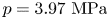 ${p}=3.97\ \textrm {MPa}$) predicted by the PR equation-of-state without a volume translation model (PR) and with the volume translation model, proposed by Abudour et al. (Reference Abudour, Mohammad, Robinson and Gasem2012) (PRVT) with the NIST database. It is not surprising that the discrepancies of PRVT from the NIST database are higher than the discrepancies between the PR and the NIST database, since the volume translation model is optimized for the near-critical conditions. Figure 20 also compares the thermodynamic and the transport properties predicted by the present methods with the PR and PRVT equation-of-states and Chung et al. correlations for nitrogen at
  ${p}=3.97\ \textrm {MPa}$. The optimized model constants are presented in table 2. Here, the absolute deviations of the predicted values from the NIST database are presented in the legend. The results show that the present modifications considerably reduce the discrepancies of the PR equation-of-state and Chung et al. correlation from the NIST database. However, since the main objective of the present paper is to study the effects of the excitations on the supercritical jet, the excitations induce pressure oscillations in the computational domain. Therefore, it is mandatory to validate the modified models at other pressures. The present simulations of the excited cases show that the pressure fluctuations in the entire computational domain do not exceed 0.5 % of the mean pressure during the excitations. For such pressure range, the maximum and mean values of AD for all the predicted properties are less than 1.8 % and 0.5 %, respectively.
Table 2. Optimized model constants.


Figure 20. Nitrogen; (a) density, (b) constant pressure heat capacity, (c) viscosity and (d) thermal conductivity versus temperature at 3.97 Mpa. The maximum and average values of the AD of the predicted variables from the NIST database are presented in the legends.


