


1 Introduction
It might seem that eddy resolving simulation of turbulent flow over rough walls requires the geometry of the roughness to be represented explicitly: the turbulence contains eddies created by the roughness elements; apparently, geometrical asperities must be present to create these eddies. Such a requirement would appear to preclude wall-modelled large eddy simulation (LES), or detached eddy simulation (DES). That will be shown, herein, to be too pessimistic.
Quite interestingly, the dominant, large eddies, seen over rough walls, do not depend on the presence of geometrical elements. They form in the mean shear. Rough surfaces break up the streaks that are seen over smooth walls; but, remarkably, that too does not require the geometrical elements. In both cases, it is necessary to model the form drag on the rough wall, but a rough geometry is not necessary. In a sense, the primary result of the present paper is to show that an expanded concept of the ‘Townsend hypothesis’ (Townsend Reference Townsend1976) is applicable to eddy resolving simulation.
The Townsend hypothesis is that, beyond a few roughness heights from the wall, the Reynolds stresses scale on friction velocity, irregardless of whether the wall is rough or smooth. Flack, Schultz & Shapiro (Reference Flack, Schultz and Shapiro2005) confirmed experimentally, that the Reynolds stresses for two types of surface roughness agree, above  $3k_{s}$, with those on smooth wall, when both are scaled on friction velocity. Here,
  $k_{s}$ is equivalent sand-grain roughness. All the stresses scale, and are independent of the specific roughness geometry.
A corollary to Townsend’s hypothesis is that roughness can be replaced by a force that produces the same drag as the geometrical roughness. For a given bulk flow Reynolds number, the same drag means the same friction coefficient. Hence, the Reynolds stresses will be captured by the force model, under the same flow conditions as the rough wall. Here, this corollary to Townsend’s hypothesis is extended to show that large scale turbulence structures are captured, as well as the Reynolds stresses. Even further, the drag force breaks up wall streaks in a similar manner to geometrical roughness. The latter is quite striking; it provides a new perspective on the action of surface roughness.
Two methods have been used to represent roughness in Reynolds averaged modelling without resolving the geometry: a boundary condition (Knopp, Eisfeld & Calvo Reference Knopp, Eisfeld and Calvo2009) or a distributed force (Stripf et al. Reference Stripf, Schulz, Bauer and Wittig2009). The boundary condition is not attractive for eddy resolving simulation; indeed, that was explored very briefly and found to be unsuitable. The distributed force is less popular in Reynolds-averaged Navier–Stokes (RANS) models, but is more attractive for present purposes. The force is a quadratic drag, times a shape function of wall distance (Stripf et al. (Reference Stripf, Schulz, Bauer and Wittig2009), provide a literature survey, dating back to Schlichting in 1936). Busse & Sandham (Reference Busse and Sandham2012) applied the quadratic drag model to eddy resolving simulations. They explored a variety of shape functions, in direct numerical simulations. Their results show that this is a viable method to represent surface roughness effects on turbulent flow. The present paper explores the implications of using this model, devised for Reynolds averaged computation, in eddy resolving simulations.
The quadratic drag model was also studied by Krumbein et al. (Reference Krumbein, Forooghi, Jakirlić, Magagnato and Frohnapfel2017) in the context of very large eddy simulation. They evaluated the drag coefficient, as a function of wall distance, from complementary DNS simulations. In the meteorological literature, starting with Shaw & Schumann (Reference Shaw and Schumann1992), the drag model has been used to represent plant canopies in LES. In that context the drag coefficient, homogeneous in streamwise direction, is only a function of wall distance and is attributed to leaf area density. Yue et al. (Reference Yue, Parlange, Meneveau, Zhu, van Hout and Katz2007) review this application and describe a model that approximately takes into account the spatial arrangement and morphology of the plants. Thereby, the drag term includes a distributed force contribution from both leaves and stems. In those studies the flow both above and within the plant canopy is of interest.
2 Roughness model
The surface roughness is modelled by introducing a momentum sink  $f_{i}$ in the incompressible, filtered Navier–Stokes equation
 $$\begin{eqnarray}\displaystyle \frac{\unicode[STIX]{x2202}\hat{u} _{i}}{\unicode[STIX]{x2202}t}+\hat{u} _{j}\frac{\unicode[STIX]{x2202}\hat{u} _{i}}{\unicode[STIX]{x2202}x_{j}}=-\frac{1}{\unicode[STIX]{x1D70C}}\frac{\unicode[STIX]{x2202}\hat{p}}{\unicode[STIX]{x2202}x_{j}}+\frac{\unicode[STIX]{x2202}}{\unicode[STIX]{x2202}x_{j}}\left(\unicode[STIX]{x1D708}\frac{\unicode[STIX]{x2202}\hat{u} _{i}}{\unicode[STIX]{x2202}x_{j}}-\unicode[STIX]{x1D70F}_{ij}^{SGS}\right)-f_{i}, & & \displaystyle\end{eqnarray}$$
 where  $\hat{u} _{i}$ is the filtered velocity field,
  $\hat{p}$ is the pressure field,
  $\unicode[STIX]{x1D70F}_{ij}^{SGS}$ is the subgrid stress,
  $\unicode[STIX]{x1D70C}$ is the density and
  $\unicode[STIX]{x1D708}$ is the kinematic viscosity of fluid. Here,
  $\unicode[STIX]{x1D70F}_{ij}^{SGS}$ is closed by linearly relating it to the filtered rate of strain
  $\widehat{S}_{ij}$,
 $$\begin{eqnarray}\unicode[STIX]{x1D70F}_{ij}^{SGS}=-2\unicode[STIX]{x1D708}_{t}\widehat{S}_{ij}+{\textstyle \frac{1}{3}}\unicode[STIX]{x1D6FF}_{ij}\unicode[STIX]{x1D70F}_{kk}^{SGS}\end{eqnarray}$$
 as in linear eddy viscosity models. The eddy viscosity  $\unicode[STIX]{x1D708}_{t}$ is defined as per the adaptive, delayed detached eddy simulation (DDES) model of Reddy, Ryon & Durbin (Reference Reddy, Ryon and Durbin2014). The version of the DDES model used in the current study is outlined in Yin & Durbin (Reference Yin and Durbin2016). It makes use of the dynamic procedure to minimize the subgrid viscosity on well-resolved grids. On the present grids, simulations with this model are equivalent to wall-resolved LES.
The sink term is active in a volume zone, called the ‘roughness zone’, that extends from the surface up to a wall-normal distance of  $k_{p}$ (figure 1), where
  $k_{p}$ is the mean-peak height of the rough surface. Here,
  $f_{i}$ is quadratically proportional to a local velocity scale
  $u_{rz}$, and included only for the cells in the roughness zone. The velocity scale is constant along each wall-normal linelet, and equal to the instantaneous velocity at the upper edge of the roughness zone. Specifically,
  $u_{rz,i}[cell_{m}]=\hat{u} _{i}[cell_{n}]$ when the wall tangential distance between
  $cell_{m}$ and
  $cell_{n}$ is less than the cube root of the volume of
  $cell_{m}$. This definition is tailored to unstructured grids. It is stated mathematically as
 $$\begin{eqnarray}|(\boldsymbol{x}_{c,m}-\boldsymbol{x}_{c,n})-[(\boldsymbol{x}_{c,m}-\boldsymbol{x}_{c,n})\boldsymbol{\cdot }\hat{\boldsymbol{n}}_{m}]\hat{\boldsymbol{n}}_{m}|<{V_{m}}^{1/3}.\end{eqnarray}$$
 Here,  $\hat{n}_{m}$ is the surface-normal unit vector,
  $\boldsymbol{x}_{c,m}$ is the coordinate vector of the centre of
  $cell_{m}$ and
  $V_{m}$ is the volume of
  $cell_{m}$. Cells at the top of the forcing region are found amongst the cells in the roughness zone by the condition that
  $(k_{p}-d_{w}[cell_{n}])$ is a minimum, where
  $d_{w}$ is the wall distance. The forcing term is defined as
 $$\begin{eqnarray}\boldsymbol{f}=\unicode[STIX]{x1D6FC}_{t}|\boldsymbol{u}_{rz}|\boldsymbol{u}_{rz,t}+\unicode[STIX]{x1D6FC}_{n}|\boldsymbol{u}_{rz}|\boldsymbol{u}_{rz,n},\end{eqnarray}$$
 where  $\unicode[STIX]{x1D6FC}$ determines the intensity of the forcing term, and
  $\langle \cdot \rangle _{t}$ and
  $\langle \cdot \rangle _{n}$ are the wall-tangential and normal components, respectively. For present purposes the normal component is not needed,
  $\unicode[STIX]{x1D6FC}_{n}=0$, and a constant value of
  $\unicode[STIX]{x1D6FC}_{t}$ is sufficient to capture the effects of roughness in the outer region. The rationale for the model (2.4) can be found in Stripf et al. (Reference Stripf, Schulz, Bauer and Wittig2009). The forcing term could also be expressed in a generalized form as
 $$\begin{eqnarray}f_{i}=\unicode[STIX]{x1D6FC}_{ij}|\boldsymbol{u}_{rz}|u_{rz,j},\end{eqnarray}$$
 where  $\unicode[STIX]{x1D6FC}_{ij}=\text{diag}\{\unicode[STIX]{x1D6FC}_{t},\unicode[STIX]{x1D6FC}_{t},\unicode[STIX]{x1D6FC}_{n}\}$ in (2.4), whereas
  $\unicode[STIX]{x1D6FC}$ was isotropic,
  $\unicode[STIX]{x1D6FC}_{ij}=\unicode[STIX]{x1D6FC}\unicode[STIX]{x1D6FF}_{ij}$, and a function of wall distance in Shaw & Schumann (Reference Shaw and Schumann1992). Anisotropic
  $\unicode[STIX]{x1D6FC}_{ij}$ should be more appropriate for modelling the drag of surface roughness.
The forcing term is made proportional to  $\boldsymbol{u}_{rz}$, instead of the local velocity
  $\tilde{\boldsymbol{u}}$, to ensure that the roughness form drag always acts in the direction opposing the bulk flow over the roughness zone. Therefore, this model can reproduce the mild separated region in the averaged streamwise flow obtained for extremely rough surfaces like transverse square-rib roughened walls (Leonardi et al. Reference Leonardi, Orlandi, Smalley, Djenidi and Antonia2003; Ikeda & Durbin Reference Ikeda and Durbin2007; Ismail, Zaki & Durbin Reference Ismail, Zaki and Durbin2018b). Note that this differs from Busse & Sandham (Reference Busse and Sandham2012) who used local velocity in (2.4), and who found that the tensorially correct form
  $|\boldsymbol{u}|$ impaired outer layer similarity, so they used the magnitude of a component
  $|\boldsymbol{u}_{i}|$. The present formulation is tensorially consistent and produces quite satisfactory outer layer results.

Figure 1. (a) Schematic of actual rough surface and (b) the corresponding volume-forcing zone on a smooth wall for modelling its effect.
3 Solver details
The open-source software, OpenFOAM 2.4.0 was used for all the simulations in the current study. The pressure–velocity equations were solved by the PISO (pressure-implicit with splitting of operators) algorithm, with two corrector steps. Gaussian finite volume integration with linear interpolation (second-order accurate) was employed for spatial discretization. The Sweby limiter was applied on the advective terms of the  $k$ and
  $\unicode[STIX]{x1D714}$ equations. A second-order, implicit, finite difference scheme was used for temporal discretization. The matrix system of the pressure equation was solved by the generalized geometric-algebraic multigrid method, with Gauss–Seidel as the smoother. The
  $U$,
$U$,  $k$ and
  $\unicode[STIX]{x1D714}$ equations were solved by the symmetric Gauss–Seidel method.
4 Cube-roughened channel
The merits of the roughness model are evaluated by comparing simulation with the model to simulation of a cube-roughened surface, and to simulation of a smooth surface in § 4.2. The geometry is fully developed channel flow. First, a DDES simulation of a channel with resolved cube roughness was validated by comparison to the DNS of Ismail (Reference Ismail2018) in § 4.1.
4.1 Validation
The bottom wall is roughened with a staggered array of wall-mounted cubes and the top wall is smooth. The spacing between the cubes in streamwise,  $x$, and spanwise,
  $z$, directions is
  $w_{x}=w_{z}=k$, where
  $k$ is the length of the cube’s edge. The ratio of channel half-height to roughness height is
  $\unicode[STIX]{x1D6FF}/k=5.5$. The computational box is of size
  $(L_{x},\,L_{y},\,L_{z})=(44k,\,11k,\,20k)$. The bulk Reynolds number is maintained at
  $Re_{b}=U_{b}2\unicode[STIX]{x1D6FF}/\unicode[STIX]{x1D708}=5600$, where
  $U_{b}$ is the averaged streamwise bulk velocity. The flow at the inlet is recycled from the downstream plane at
  $x=L_{rc}=40k$ to simulate a fully developed flow. Uniform grid spacing is used in the
  $x$ and
  $z$ directions with
  $\unicode[STIX]{x0394}x/k=\unicode[STIX]{x0394}z/k=1/6$. (The DNS simulation used a much finer resolution,
  $\unicode[STIX]{x0394}x/k=\unicode[STIX]{x0394}z/k=1/10$.) The grid is stretched in the wall-normal,
  $y$, direction with
  $\unicode[STIX]{x0394}y_{r,1}^{+}=1.53$ and
  $\unicode[STIX]{x0394}y_{r,max}^{+}=15.05$, where
  $\unicode[STIX]{x0394}y_{1}$ is the height of the first cell next to the wall. There is no additional clustering of cells near the top of the cubes. In plus units, the
  $x$ and
  $z$ resolutions are
  $\unicode[STIX]{x0394}x_{r}^{+}=\unicode[STIX]{x0394}z_{r}^{+}=10.19$. Friction velocity,
  $u_{\star ,r}$, of the rough wall is used for plus units scaling. Here,
  $u_{\star ,r}$ includes contributions from both skin friction drag and pressure drag on the roughness elements. The flow statistics (mean velocity and Reynolds stress) are averaged over
  $68L_{rc}/U_{b}$ time units, and over the periodic directions,
  $x$ and
  $z$.
$z$.
Figure 2(a) shows a good agreement of viscous stress,  $(1/Re_{b})\unicode[STIX]{x2202}U/\unicode[STIX]{x2202}y$, with DNS above the rough-wall side of channel, where
  $U$ is the mean velocity in the
  $x$ direction. The root-mean-square (r.m.s.) of the fluctuating velocities,
  $u_{rms}$,
  $v_{rms}$ and
  $w_{rms}$ are also accurately predicted in most of the channel except the region within the cube roughness (figure 2b). In figure 2, velocities are scaled with
  $U_{b,s}$ to be consistent with the data from Ismail (Reference Ismail2018). Here,
  $U_{b,s}$ is defined as the bulk velocity of a narrower channel (
 $L_{y}=10k$) with the same mass-flow rate as the present case:
  $U_{b,s}=1.1U_{b}$. The friction Reynolds number on the smooth-wall side,
  $Re_{\unicode[STIX]{x1D70F},s}=u_{\star ,s}l_{m}/\unicode[STIX]{x1D708}=128.67$, is underpredicted by 4.7 %. Here,
  $l_{m}$ is the distance between the top wall and the location of
  $U_{max}$. Overall, the level of agreement between DNS and the present DDES simulation is good.

Figure 2. Validation of cube-roughened channel flow. (a) Profile of viscous stress  $[(2\unicode[STIX]{x1D6FF}-k)/(2.25U_{b,s}Re_{b})]\unicode[STIX]{x2202}U/\unicode[STIX]{x2202}y$, (b) profiles of scaled r.m.s. fluctuation-velocity components. Circles denote the DNS data from Ismail (Reference Ismail2018).
4.2 Simulation set-up
All simulations are at the same  $Re_{b}$ and on the same grid. For computations with resolved cubes, cubes were created by blanking out the portion of the grid inside the cubes. Cube roughness in channel flow has been studied by DNS in Orlandi & Leonardi (Reference Orlandi and Leonardi2006), Leonardi & Castro (Reference Leonardi and Castro2010) and Ismail, Zaki & Durbin (Reference Ismail, Zaki and Durbin2018a), among others.
The cube-roughened channel (CR) is constructed by mounting an array of identical cubes on both the top and bottom walls of the channel (figure 3). The dimension of a cube is  $k$, with streamwise and spanwise spacing
  $w_{x}=w_{z}=2k$ between the cubes. The adjacent rows of cubes in the
  $x$ direction are staggered by
  $1.5k$ in the
  $z$ direction. The plan area density of this cube arrangement is
  $\unicode[STIX]{x1D706}_{p}=1/9$, where
  $\unicode[STIX]{x1D706}_{p}$ is the ratio of the area occupied by cubes to the area of a repeating unit (figure 3). The size of the repeating unit (RU) is
  $l_{RU,x}\times l_{RU,z}=6k\times 3k$. The roughness height is
  $k/\unicode[STIX]{x1D6FF}=1/12$.
The height of the roughness zone,  $k_{p}$ in the roughness model (RM), is set at
  $k$, since all the cubes are of identical height. The grid is Cartesian, so the linelets (2.3) become, simply, constant
  $x$ and
  $z$ and
  $y<k$.
The cube-roughened channel, RM and smooth channel (SM) cases were simulated in a computational box of dimensions  $(L_{x},\,L_{y},\,L_{z})=(6.5\unicode[STIX]{x1D6FF},\,2\unicode[STIX]{x1D6FF},\,2.5\unicode[STIX]{x1D6FF})$, with
  $(N_{x},\,N_{y},\,N_{z})=(468,170,180)$ grid points. The simulations were run at
  $Re_{b}=40\,000$. The flow at the inlet was recycled from the downstream plane at
  $x=L_{rc}=6\unicode[STIX]{x1D6FF}$ to create fully developed turbulent flow. Periodic boundary conditions were imposed on the side planes in the spanwise direction. A no-slip boundary condition was applied on the top and bottom walls, and on the surfaces of the cubes.

Figure 3. Plan view of cube-roughened wall.
The grid spacing was uniform in the  $x$ and
  $z$ directions and geometrically stretched in the
  $y$ direction, with cells clustered close to both walls. The cubes in CR are resolved with six cells in both
  $x$ and
  $z$. Grid convergence with respect to the resolution in the region of cubic roughness elements is discussed in appendix A. The friction velocity,
  $u_{\star }$, is defined to include contributions from both skin friction and form drag on the roughness elements. Therefore, it was calculated from the pressure drop between the inlet plane
  $(x=0)$ and recycling plane
  $(x=L_{rc})$
 $$\begin{eqnarray}u_{\star }^{2}=\frac{1}{2\unicode[STIX]{x1D70C}L_{rc}}\int _{0}^{2\unicode[STIX]{x1D6FF}}(P_{0}-P_{L_{rc}})\,\text{d}y,\end{eqnarray}$$
 where  $P$ is the average of
  $\hat{p}$. The averaging is done over time and
  $z$. In the CR case, the
  $x$ direction pressure-drop profiles, within the repeating units close to the inlet and recycling plane, showed large differences with corresponding profiles in the midsection of the channel. Therefore,
  $u_{\star }$ for CR was calculated from pressure drop between
  $x=24k{-}66k$ instead of
  $x=0-L_{rc}$ as was done for RM and SM.
The flow statistics in RM and CR cases were averaged for  $75L_{rc}/U_{b}$ time units, whereas the SM case was averaged for
  $100L_{rc}/U_{b}$ time units. The details of the temporal and spatial resolution are summarized in table 1. The same grid, in
  $\unicode[STIX]{x1D6FF}$ scaling, was used for the three simulations being discussed, with no additional clustering around
  $y=k$ in CR or
  $y=k_{p}$ in
  $RM$. This is justified in the CR case, by the validation study in § 4.1, where the lack of clustering near top of the cubes was found to have little impact on the statistics in the outer flow. The insensitivity of the flow to the wall-normal resolution inside the roughness zone, for the modelled roughness case, is discussed in appendix B. Based on the resolution, the simulations fall in the category of wall resolved LES. On average,
  $\unicode[STIX]{x1D708}_{t}/\unicode[STIX]{x1D708}<0.35$ for RM and CR in the outer region, over the roughness-zone/cube-roughness, while it is lower by a factor of 3 for SM (figure 4). This ratio is higher near the top of the cubes in the CR case, because of the thin shear layer that separates from the cubes. However, it is still below unity.
5 Results
5.1 Roughness sublayer
The presence of roughness elements (CR case) produces a region of spatial inhomogeneity above them, in the wall-normal direction, called the roughness sublayer (RSL). The profiles of mean streamwise velocity, averaged in  $z$, at different
  $x$ locations (within the repeating unit of roughness elements) are compared with the profile averaged in both
  $x$ and
  $z$, in figure 5. The variation near the wall is caused by the wake of the cubes. The roughness sublayer is defined as the region where there is inhomogeneity in
  $x$. As per figure 5, RSL extends to
  $y/k=2$. This is a typical estimate of the roughness sublayer, but it can be seen that most of the profiles differ little from the profile averaged in
  $x$ and
  $z$. Ismail et al. (Reference Ismail, Zaki and Durbin2018a) reported a similar extent of RSL up until
  $2k{-}2.5k$. For the most part, the rough geometry does not create a substantial obstruction. For many purposes, the height of the roughness sublayer is little more than
  $y/k=1$. For an array of rectangular prisms of random height, Yang et al. (Reference Yang, Sadique, Mittal and Meneveau2016) found the depth of the roughness layer to be very nearly the height of the highest elements. On the other hand, RM does not have a roughness sublayer because the roughness zone has no underlying spatial inhomogeneity.
Table 1. Grid resolution in plus units and Kolmogorov scale ratios. Here,  $\unicode[STIX]{x0394}y_{1}$ is the height of the cell height next to the wall,
  $\unicode[STIX]{x0394}y_{max}$ is the maximum cell height,
  $\unicode[STIX]{x1D702}$ is the Kolmogorov length scale and
  $\unicode[STIX]{x1D70F}_{\unicode[STIX]{x1D702}}$ is the Kolmogorov time scale.


Figure 4. Ratio of subgrid-scale viscosity to molecular viscosity. The vertical dashed line denotes the height of roughness,  $k/\unicode[STIX]{x1D6FF}=1/12$.

Figure 5. Profiles of spanwise-averaged mean streamwise velocity in CR case.
5.2 Instantaneous velocity field
The roughness model is able to produce elevated velocity fluctuations, relative to the smooth channel, similar to resolved cube roughness, at the same bulk Reynolds number,  $Re_{b}$. In the side view of figure 6, CR and RM have similar appearances. A difference is noticeable very near the wall, within the region containing cubes; but, the large eddies are of roughly similar intensity and size. This will be substantiated, below, by Reynolds stresses and spatial spectra.

Figure 6. Contours of  $u^{\prime }/U_{b}$ at
  $z/\unicode[STIX]{x1D6FF}=1.5$ (side view). Contour levels: blue,
  $-0.25$; green, 0; red, 0.25.
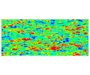
The plan view is more remarkable. The elongated streaks seen in the buffer region of SM, figure 7(c), are broken down in both the RM and CR cases of figure 7(a,b). This is an extraordinary result. Do the cubes break up streaks because they are a physical obstruction, because they generate eddies in their wakes; or is breakup due to form drag, exerted as a body force? Figure 7(a), compared to 7(c), shows how form drag alone can break up streaks. Indeed, figures 7(a) and 7(b) are strikingly similar, given that there are no cubes present in the former. A simple explanation is that the high-speed streaks are strongly damped by the form drag (2.4). Quadratic dependence on velocity suppresses high-speed streaks. Busse & Sandham (Reference Busse and Sandham2012) also noted a weakening of the streaks that are seen over smooth walls, when they introduced a drag layer.
The top views, just discussed, were inside the roughness zone. Elevated velocity fluctuations, relative to SM, are also observed in the RM and CR cases of figure 8, at a wall-normal plane above the roughness,  $y/k=2.02$ or
  $y/\unicode[STIX]{x1D6FF}=0.17$. The large eddies are similar for RM and CR in figure 8. Figure 9 is higher above the wall, at
  $y/k=4.13$,
  $y/\unicode[STIX]{x1D6FF}=0.34$. This is in the outer region, outside the roughness sublayer. Both CR and RM are virtually indistinguishable.
Townsend (Reference Townsend1976) postulated that if the roughness layer is much thinner than the boundary layer  $(k\ll \unicode[STIX]{x1D6FF})$, effects of roughness would be limited to the inner region, while, in the outer region, the rough flow should be structurally similar to smooth flow. Specifically, that roughness would only modify the velocity scale
  $(u_{\star })$, and that the Reynolds stress profiles would collapse, when normalized by
  $u_{\star }$. That normalization is applied to the instantaneous fields in figures 10 and 11. The side view of SM, figure 10(c), perhaps shows more evidence of streaks near the wall, than the CR and RM panels, 10(a) and 10(b); but, the similarity of the scaled plots largely explains why the simple forcing model produces proper levels of velocity fluctuation: they scale on
  $u_{\star }$.
The top view, figure 11, is in the outer region. The contours of  $u^{\prime }$, scaled by
  $u_{\star }$, are similar in the three cases. However, the smooth-wall contours have less small-scale variation than the other two. That can be attributed to
  $Re_{\unicode[STIX]{x1D70F}}$ being lower for SM, as will be explained below. In this vein, one could expand on Townsend’s hypothesis: beyond a few roughness heights from the wall, the Reynolds stresses scale on friction velocity, and the turbulence has a similar spectrum of scales for a given
  $Re_{\unicode[STIX]{x1D70F}}$, regardless of whether the wall is rough or smooth. In figure 11 the bulk Reynolds numbers are all the same, and
  $Re_{\unicode[STIX]{x1D70F}}$ for the SM case is approximately half that of RM and CR. The smooth case does not satisfy the expanded hypothesis; that is why it has less small-scale structure.

Figure 7. Contours of  $u^{\prime }/U_{b}$ at
  $y/\unicode[STIX]{x1D6FF}=0.017$ (top view). Contour levels: blue,
  $-0.2$; green, 0; red, 0.2.

Figure 8. Contours of  $u^{\prime }/U_{b}$ at
  $y/\unicode[STIX]{x1D6FF}=0.17$ (top view). Contour levels: blue,
  $-0.3$, green, 0; red, 0.3.

Figure 9. Contours of  $u^{\prime }/U_{b}$ at
  $y/\unicode[STIX]{x1D6FF}=0.34$ (top view). Contour levels: blue,
  $-0.3$; green, 0; red, 0.3.

Figure 10. Contours of  $u^{\prime }/u_{\star }$ at
  $z/\unicode[STIX]{x1D6FF}=1.5$ (side view). Contour levels: blue,
  $-2.5$; green, 0; red, 2.5.

Figure 11. Contours of  $u^{\prime }/u_{\star }$ at
  $y/\unicode[STIX]{x1D6FF}=0.34$ (top view). Contour levels: blue,
  $-3$; green, 0; red, 3.
5.3 Mean streamwise velocity and Reynolds stresses
The instantaneous views already make a compelling case for the drag model. The Reynolds stresses are consistent with those observations. The flow statistics (mean velocity and Reynolds stress) are averaged additionally in the  $x$ and
  $z$ directions (periodic directions for CR and homogeneous directions for RM and SM), and about the channel centreline.
The log-layer slope in both CR and RM cases deviates from  $1/\unicode[STIX]{x1D705}$ (
 $\unicode[STIX]{x1D705}=0.41$) as shown in figure 5. This was also observed in the DNS of cube-roughened channel flow by Ismail et al. (Reference Ismail, Zaki and Durbin2018a) and Leonardi & Castro (Reference Leonardi and Castro2010). To be able to calculate the equivalent sand-grain roughness,
  $k_{s}$, by comparing to the log-law in the fully rough regime of experiments by Nikuradse (Reference Nikuradse1950), an effective origin
  $d$ is introduced such that slope in the log-layer is equal to
  $1/\unicode[STIX]{x1D705}$ (figure 12b). For this plot,
  $d/k=0.12$ for RM and
  $d/k=0.47$ for CR. The values reported by Ismail et al. (Reference Ismail, Zaki and Durbin2018a) and Leonardi & Castro (Reference Leonardi and Castro2010) for the same cube arrangement,
  $\unicode[STIX]{x1D706}_{p}=1/9$, are close at
  $d/k=0.6$. The constant (
 $\unicode[STIX]{x1D6FC}$) in the forcing function was chosen to obtain log-layer displacement
  $\unicode[STIX]{x0394}U^{+}$ close to that of the CR case (figure 12b); in other words, the model was calibrated to have the same equivalent sand-grain roughness as the resolved cubes. The normalized value was
  $\unicode[STIX]{x1D6FC}_{t}\unicode[STIX]{x1D6FF}=0.42$; because
  $k_{p}=\unicode[STIX]{x1D6FF}/12$, this is the same as
  $\unicode[STIX]{x1D6FC}_{t}k_{p}=0.035$. With this
  $\unicode[STIX]{x1D6FC}_{t}$, the friction velocity
  $u_{\star }$ in the RM case was within 1.5 % of that obtained in the CR case. The corresponding friction Reynolds numbers
  $Re_{\unicode[STIX]{x1D70F}}$ for RM, CR and SM are 2,112, 2,144 and 966, respectively. The equivalent sand-grain roughness for RM is
  $k_{s}^{+}=656$, 5 % higher than CR. The roughness length scale ratio
  $k_{s}/k=3.49$ in the CR case. This differs from the value of
  $k_{s}/k=2.53$ in Ismail et al. (Reference Ismail, Zaki and Durbin2018a) at fully rough condition and the same
  $\unicode[STIX]{x1D6FF}/k$ and cube density,
  $\unicode[STIX]{x1D706}_{p}$. The difference must be because of the asymmetric channel (rough lower wall and smooth upper wall) in Ismail et al. (Reference Ismail, Zaki and Durbin2018a). A rough half-channel at the same
  $\unicode[STIX]{x1D706}_{p}$ but lower
  $\unicode[STIX]{x1D6FF}/k=8$ in Leonardi & Castro (Reference Leonardi and Castro2010) results in a lower
  $k_{s}/k=2.38$ compared to CR. These studies would seem to imply that
  $k_{s}/k$, function of roughness parameters, shows a dependence on
  $\unicode[STIX]{x1D6FF}/k$ at lower ratios, around
  $\unicode[STIX]{x1D6FF}/k=10$.
Figure 13 shows the collapse in the outer region, beyond  $y/k=4$,
  $y/\unicode[STIX]{x1D6FF}=0.33$, of the streamwise velocity in defect form for RM, CR and SM. Similarly, the Reynolds stresses also collapse in the outer region for all three cases when scaled on
  $u_{\star }$ (figure 14). Near the wall
  $\overline{u^{^{\prime }2}}^{\,+}$ has a pronounced peak for SM, which is absent for RM and CR; indeed, RM reproduces the behaviour of CR quite closely. The presence of a peak for SM is due to the intense streaks seen in figure 7(c). The absence of a peak for RM and CR supports the evidence in figure 7(a,c), that the model breaks up the streaky structure. The essential attribute of surface roughness is not geometrical obstruction, but form drag. It is remarkable that the effect on turbulence structure can be represented by a layer of quadratic drag force. The scaled wall-normal component
  $\overline{v^{,2}}^{\,+}$ for RM is also close to CR and SM in the outer region.

Figure 12. Profiles of mean streamwise velocity in outer and inner scaling. The vertical dashed line denotes the height of roughness,  $k/\unicode[STIX]{x1D6FF}=1/12$.

Figure 13. Profiles of mean streamwise velocity in velocity-defect form. Here,  $U_{c}$ is the centreline velocity. The vertical dashed line denotes the height of roughness,
  $k/\unicode[STIX]{x1D6FF}=1/12$.

Figure 14. Profiles of Reynolds stress components in plus units. The vertical dashed line denotes the height of roughness,  $k/\unicode[STIX]{x1D6FF}=1/12$.
5.4 Energy spectra
Scaled energy spectra in the  $x$ direction are shown in figures 15 and 16. The large scale structures, of size greater than the channel half-width
  $(\unicode[STIX]{x1D705}_{x}\unicode[STIX]{x1D6FF}<2\unicode[STIX]{x03C0})$, have lower energy in the CR case than in the SM case, at height
  $y/k=2.02$,
  $y/\unicode[STIX]{x1D6FF}=0.17$ (figure 15). The drag model does not damp these very large scales and lies close to the smooth-wall simulation; however, these very long streamwise scales are influenced by the length of the computational domain and are not integral to turbulent transport.
In the more important range of scales, between  $\unicode[STIX]{x1D6FF}$ and
  $k$, demarcated by vertical dashed lines in figure 15, all of the
  $E_{uu}$ collapse when scaled on
  $u_{\star }$. Volino, Schultz & Flack (Reference Volino, Schultz and Flack2007) also found a similarity between scaled energy spectra in the outer region of rough- and smooth-wall flow at scales smaller than
  $\unicode[STIX]{x1D6FF}$ but larger than
  $k$. The striking result is the similarity between RM and CR at scales smaller than the roughness height,
  $k$. The SM has low energy at these scales, while RM remains higher, following CR.
Higher above the wall, in the outer region, at  $y/\unicode[STIX]{x1D6FF}=0.34$, figure 16 shows a very strong agreement between RM and CR, and a clear distinction from SM. This corresponds to figure 11, in which the instantaneous velocity contours produced by the model are visibly like those produced from the simulation with resolved cubes. But, how can the drag model produce small scales of turbulence? That question shows a misunderstanding of the effect of roughness. The increased wall stress requires a larger pressure drop to achieve a given bulk velocity. The mean flow profile has larger shear in the outer region, as seen in figure 12(a). The spectrum represents production of turbulence by the mean shear, not by roughness.
The scaled energy spectra in the  $z$ direction for RM, shown in figures 17 and 18 at
  $y/\unicode[STIX]{x1D6FF}=2.02$ and
  $y/\unicode[STIX]{x1D6FF}=4.13$, collapse with CR for length scales smaller than
  $\unicode[STIX]{x1D6FF}$, in a similar fashion to the energy spectra in the
  $x$ direction. Similarly, the spectra for SM collapse with RM and CR in the intermediate range of scales and falls off at the higher spanwise wavenumbers,
  $k_{z}$.
One can consider an enlarged ‘Townsend hypothesis’. The basic hypothesis is that scaling velocity on  $u_{\star }$ will collapse the Reynolds stresses. That does not collapse the spectra. The simulations all have the same
  $Re_{b}$ but SM has a lower
  $Re_{\unicode[STIX]{x1D70F}}$ than RM and CR. The enlarged hypothesis is that the energy spectra scale on
  $u_{\star }$, but will collapse if they also have the same friction Reynolds number. The rough-wall
  $Re_{\unicode[STIX]{x1D70F}}$ is too high for us to afford a smooth-wall simulation at the same Reynolds number. In figure 19(a), data from smooth-wall DNS by Lee & Moser (Reference Lee and Moser2015) at
  $Re_{\unicode[STIX]{x1D70F}}=1000$ and
  $Re_{\unicode[STIX]{x1D70F}}=2000$ are compared to the present simulations. The DNS have more energy at the shortest wavelengths because they are on highly resolved grids. However, in the range between the two vertical lines, the smooth-wall spectra confirm that the dominant effect is the higher
  $Re_{\unicode[STIX]{x1D70F}}$ caused by drag on the roughness.
Having established the outer similarity of energy spectra, in outer scaling, between smooth wall and rough wall (both CR and RM), the collapse of spectra in the dissipation range can be verified in Kolmogorov scaling. As expected, the spectra for the three cases (different  $Re_{\unicode[STIX]{x1D70F}}$) have an acceptable collapse in the universal equilibrium range as shown in figure 19(b). The noticeable discrepancy in the inertial subrange is because LES does not provide dissipation rate (
 $\unicode[STIX]{x1D716}$) of turbulent kinetic energy, so it had to be estimated. The estimation is more inaccurate on the coarse grids in RM and CR, compared to SM.

Figure 15. Energy spectra in the  $x$ direction at
  $y/\unicode[STIX]{x1D6FF}=0.17$ (
 $y_{s}^{+}=163$,
  $y/k=2.02$). The vertical lines denote the length scales: – –, channel half-width (
 $\unicode[STIX]{x1D6FF}$);
  $\cdots \,$, roughness (
 $k$).
$k$).

Figure 16. Energy spectra in the  $x$ direction at
  $y/\unicode[STIX]{x1D6FF}=0.34$ (
 $y_{s}^{+}=332$,
  $y/k=4.13$). The vertical lines denote the length scales: – –, channel half-width (
 $\unicode[STIX]{x1D6FF}$);
  $\cdots \,$, roughness (
 $k$).
$k$).

Figure 17. Energy spectra in the  $z$ direction at
  $y/\unicode[STIX]{x1D6FF}=0.17$ (
 $y_{s}^{+}=163$,
  $y/k=2.02$). The vertical lines denote the length scales: – –, channel half-width (
 $\unicode[STIX]{x1D6FF}$);
  $\cdots \,$, roughness (
 $k$).
$k$).

Figure 18. Energy spectra in the  $z$ direction at
  $y/\unicode[STIX]{x1D6FF}=0.34$ (
 $y_{s}^{+}=332$,
  $y/k=4.13$). The vertical lines denote the length scales: – –, channel half-width (
 $\unicode[STIX]{x1D6FF}$);
  $\cdots \,$, roughness (
 $k$).
$k$).

Figure 19.  $E_{uu}$ (Energy spectra) in the
  $x$ direction at
  $y/\unicode[STIX]{x1D6FF}=0.34$ (
 $y_{s}^{+}=332$,
  $y/k=4.13$) (a) in outer scaling and (b) in Kolmogorov scaling. The vertical lines denote the length scales: – –, channel half-width (
 $\unicode[STIX]{x1D6FF}$);
  $\cdots \,$, roughness (
 $k$). The grey — ⋅ — line represents the Kolmogorov
  $-5/3$ scaling law. Energy spectra from DNS of smooth channel (Lee & Moser Reference Lee and Moser2015): black — ⋅ —,
  $Re_{\unicode[STIX]{x1D70F}}=1000$; red — ⋅ —,
  $Re_{\unicode[STIX]{x1D70F}}=2000$.
6 Proper orthogonal decomposition
Proper orthogonal decomposition (POD) modes were computed in an attempt to provide a statistical corollary to the instantaneous contours of  $u^{\prime }$. Generally, this was not informative.
The POD of the streamwise velocity fluctuation  $u^{\prime }$ in the
  $x{-}y$ plane were computed by the snapshot method (Sirovich Reference Sirovich1987). Time snapshots are gathered for
  $50L_{rc}/U_{b}$ (50 through-flow times) with the time interval
  $\text{d}t=(1/72)L_{rc}/U_{b}$ between successive snapshots to ensure low correlation between them. Modes are arranged in descending order of % energy captured (eigenvalues) and corresponding mode shapes are given by the eigenvectors. The mode shapes are averaged about the channel centreline.
Low modes have wavelengths comparable to the domain length, and are not representative of turbulence structure. Figures 20 and 21 compare two more relevant modes. While the mode shapes for the forcing model are in agreement with those of the cube-resolved simulation, their discrepancy with the smooth-wall simulation is largely a slight reordering of the modes: the 5th mode for SM is like the 7th mode for RM, and vice versa. Any differences between the modes are close to the wall with the RM and CR structures existing further away from the wall compared to the wall attached structures in SM. Similar behaviour of POD modes in rough- and smooth-wall flow was also observed by Sen, Bhaganagar & Juttijudata (Reference Sen, Bhaganagar and Juttijudata2007). The POD modes provide incremental support to the spectra and instantaneous views presented previously, but are far less compelling than previous results.

Figure 20. Contours of the 5th POD mode of  $u^{\prime }$. The modes are normalized to have unit norm.

Figure 21. Contours of the 7th POD mode of  $u^{\prime }$. The modes are normalized to have unit norm.
7 Discussion
The present study demonstrates the ability of a simple drag layer to reproduce the effects of rough surfaces in the outer flow. The accurate prediction of the turbulence statistics in the outer region of surface roughness by the drag model depends on two conditions being satisfied: firstly, Townsend’s hypothesis holds for the present arrangement of cube-roughness even at large roughness heights ( $\unicode[STIX]{x1D6FF}/k=12$); and secondly, the chosen value of the model parameter (
 $\unicode[STIX]{x1D6FC}_{t}$) of the drag term, active in the inner region, fixes the velocity scale (wall stress) for the outer flow to be equal to the corresponding value in resolved roughness case. Chung, Monty & Ooi (Reference Chung, Monty and Ooi2014) have previously shown that mean wall-shear stress and wall impermeability at fixed
  $Re_{\unicode[STIX]{x1D70F}}$ are sufficient conditions to obtain outer similarity of flow statistics. The success of the simple drag layer seems to follow the observations of Chung et al. (Reference Chung, Monty and Ooi2014), and holds at much higher friction Reynolds number (
 $Re_{\unicode[STIX]{x1D70F}}\approx 2000$) and for extremely rough cases (
 $\unicode[STIX]{x0394}U^{+}\approx 12$) in the present study.
The roughness model and the approach of imposing stress boundary condition at the wall (Chung et al. Reference Chung, Monty and Ooi2014) are contrasted below. Channel flow with the roughness model (Model) is simulated at  $Re_{b}=$ 20 000. The height of the roughness zone is set to
  $k_{p}/\unicode[STIX]{x1D6FF}=0.08$ and the model constant is fixed at
  $\unicode[STIX]{x1D6FC}_{t}\unicode[STIX]{x1D6FF}=0.3$. The computational box is of size –
  $(L_{x},L_{y},L_{z})=(6\unicode[STIX]{x1D6FF},2\unicode[STIX]{x1D6FF},3\unicode[STIX]{x1D6FF})$ and discretized with a Cartesian grid –
  $(N_{x},N_{y},N_{z})=(150,130,150)$. The grid resolution in plus units are
  $\unicode[STIX]{x0394}x^{+}=2\unicode[STIX]{x0394}z^{+}=39.1$,
  $\unicode[STIX]{x0394}y_{1}^{+}=1.95$ and
  $\unicode[STIX]{x0394}y_{max}^{+}=50.73$. The resulting friction velocity and friction Reynolds number are
  $u_{\star ,m}/U_{b}=0.09768$ and
  $Re_{\unicode[STIX]{x1D70F},m}=976.84$. The stress boundary condition case (WallStrBC) is similar to the Model case except with the drag term switched off, and the no-slip boundary condition replaced with stress boundary condition and impermeability condition:
  $\unicode[STIX]{x2202}u/\unicode[STIX]{x2202}y=u_{\star ,m}^{2}/\unicode[STIX]{x1D708},~\unicode[STIX]{x2202}w/\unicode[STIX]{x2202}y=0$ and
  $v=0$. Additionally, a smooth-wall case is run on the same domain and grid to obtain a Reynolds number,
  $Re_{\unicode[STIX]{x1D70F},s}=976.66$, close to that of the Model case.
The WallStrBC is able to accurately capture the mean streamwise velocity ( $U$) in the outer region of the Model case (figure 22a). The difference lies close to the wall where
  $U$ in case of WallStrBC has a large reverse flow, up to
  $y^{+}=10$, allowed by the boundary condition that doesn’t enforce no-slip (figure 22b). Outer similarity holds for both the Model and the WallStrBC case, evident from the profiles of Reynolds stress components (figure 23). Reynolds stress components are suppressed within the roughness zone of the Model compared to the inner region of smooth-wall flow (figure 23). In § 5.3, the Reynolds stress levels inside the roughness region for modelled roughness were shown to be very close to that obtained for sparse cube roughness. On the other hand, the variation of
  $\overline{v^{^{\prime }2}}$ and
  $\overline{w^{^{\prime }2}}$ in the inner region for the WallStrBC is very similar to smooth wall expect for the non-zero value of
  $\overline{w^{^{\prime }2}}$ very near to the wall resulting from the velocity slip permitted by the gradient boundary condition. For WallStrBC,
  $\overline{u^{^{\prime }2}}$ peak is much more pronounced than smooth wall and shifted right next to the wall. Clearly, the normal components of Reynolds stress are more isotropic in the inner region of the Model similar to resolved roughness and unlike smooth wall and WallStrBC (Chung et al. Reference Chung, Monty and Ooi2014). Therefore, the drag model produces a better representation of rough wall flow.

Figure 22. Profiles of mean streamwise velocity in (a) outer and (b) inner scaling. The vertical dashed line denotes the height of the roughness zone,  $k_{p}/\unicode[STIX]{x1D6FF}=0.08$.

Figure 23. Profiles of Reynolds stress components in outer scaling. The vertical dashed line denotes the height of the roughness zone,  $k_{p}/\unicode[STIX]{x1D6FF}=0.08$.
The drag model (2.4) can be used to represent rough surfaces of varying roughness function ( $\unicode[STIX]{x0394}U^{+}$) by adjusting
  $\unicode[STIX]{x1D6FC}_{t}$. Smooth-wall results are recovered on setting
  $\unicode[STIX]{x1D6FC}_{t}=0$. The next step would be to evaluate a calibration curve in the fully rough regime between
  $\unicode[STIX]{x1D6FC}_{t}\unicode[STIX]{x1D6FF}$ and (
 $k_{s}/\unicode[STIX]{x1D6FF}$,
  $k_{p}/\unicode[STIX]{x1D6FF}$) on an LES quality grid by running a set of simulations. A fast approach for calibration would be by performing minimal channel simulations that accurately capture the near-wall flow up to part of the log-layer – the region of interest to calculate
  $k_{s}$. The above approach for characterising rough surfaces is discussed in MacDonald et al. (Reference MacDonald, Chung, Hutchins, Chan, Ooi and García-Mayoral2017). Preliminary runs have shown
  $\unicode[STIX]{x1D6FC}_{t}\unicode[STIX]{x1D6FF}$ to be independent of
  $k_{p}/\unicode[STIX]{x1D6FF}$ for
  $k_{p}/\unicode[STIX]{x1D6FF}\leqslant 0.04$ such that the function to be evaluated is
  $\unicode[STIX]{x1D6FC}_{t}k_{p}=f(k_{s}/k_{p})$. Further,
  $\unicode[STIX]{x1D6FC}_{t}k_{p}$ can be directly related to rough-surface topography through correlations between
  $k_{s}/k$ and surface statistics (Flack & Schultz Reference Flack and Schultz2010).
8 Conclusions
The motive behind the present paper is development of a method for representing the effect of surface roughness in an eddy resolving simulation. The intended usage is either large eddy simulation, perhaps with a wall model, or detached eddy simulation. Applications may include the likes of eroded turbine blades, or ship hulls with barnacles. Meshing the rough geometry is not viable in such cases.
The results presented herein are a fundamental justification for a simple approach. It has been shown that the field of turbulence above a layer of quadratic drag forcing is remarkably similar to that above a cube-roughened wall. This observation provides a new perspective on the fluid dynamical action of distributed roughness. Its dominant effect is not to create eddies in the wake of asperities. Such eddies are, indeed, created, but they have little effect on the turbulence structure above the roughness layer. Even within the roughness, where the asperities suppress streaks, that effect is attributable to form drag, rather than direct, physical disruption. A drag model, with no geometrical features, suppresses streaks in a quite similar way to resolved roughness. The streaky features, per se, are damped because high-speed streaks have long, jet-like velocity contours. Drag proportional to the jet velocity squared disproportionately damps regions of high velocity.
The hypothesis of Townsend (Reference Townsend1976) is a version of Occam’s razor: adopt the simplest solution. In present terms, the assertion of the Townsend hypothesis is that, above the region of geometrical roughness, the dominant effect of that roughness is to create drag; and, as such, Reynolds stresses collapse when scaled on friction velocity. In fact, that hypothesis is not quite correct for  $\overline{u^{^{\prime }2}}/u_{\star }^{2}$, even above a smooth wall, the scaled variance depends weakly on Reynolds number (De Graaff & Eaton Reference De Graaff and Eaton2000). For eddy resolving simulation, the Reynolds number dependence is more profound. To capture the spectrum of turbulence, a revised hypothesis is needed; beyond a few roughness heights from the wall, the spectrum of turbulence is determined, in large part, by the friction Reynolds number, irregardless of whether the wall is rough or smooth. In the present case, the drag constant,
  $\unicode[STIX]{x1D6FC}_{t}$, was selected to match the skin friction on a wall with cubic roughness, at a given bulk Reynolds number. Hence, both the bulk and friction Reynolds numbers were matched.
The expanded Townsend hypothesis explains the effectiveness of the drag model. That hypothesis is not applicable to non-equilibrium flows, such as a rough-to-smooth junction, or to a channel with one rough and one smooth wall. The purpose of this study is to rationalize the corollary, that geometrical roughness can be replaced by a quadratic drag model.
Acknowledgements
The work was funded by the Office of Naval Research, grant no. N00014-17-1-2200. Computational resources were provided by Extreme Science and Engineering Discovery Environment (XSEDE) and the Office of Naval Research.
Declaration of interests
The authors report no conflict of interest.
Appendix A. Cube roughened channel: grid convergence
The convergence of the flow statistics is studied with respect to the grid resolution in the region of roughness elements for cube-roughened channel flow. The roughness height is the same as in § 4.2 ( $k/\unicode[STIX]{x1D6FF}=1/12$). To keep the computational costs from being too high for the finest of grids, a smaller domain is used compared to § 4.2, and a half-channel is simulated with symmetry boundary conditions on the top face. The computational box is of dimensions
  $(L_{x},~L_{y},~L_{z})=(4.5\unicode[STIX]{x1D6FF},~\unicode[STIX]{x1D6FF},~\unicode[STIX]{x1D6FF})$ and the flow at the inlet is recycled from the downstream plane at
  $x=L_{rc}=4\unicode[STIX]{x1D6FF}$, ensuring
  $Re_{b}=20\,000$. The different resolutions studied are summarized in table 2. The
  $y$-grid is identical in all cases, with
  $\unicode[STIX]{x0394}y_{1}^{+}=1.84$,
  $y_{cubeTF}^{+}=6.32$ and
  $\unicode[STIX]{x0394}y_{max}^{+}=23.06$, where
  $y_{cubeTF}^{+}$ is the height of the cell next to the cube’s horizontal top face and
  $u_{\star }$ of case C12 is used for scaling. The
  $y$-grid in the region of wall mounted cubes is comparable to
  $\unicode[STIX]{x0394}x^{+}$ and
  $\unicode[STIX]{x0394}z^{+}$ of case C12. Hence, convergence of grid resolution in the
  $y$ direction is not studied.
Table 2. Grid resolutions for convergence study of cube-roughened channel.

The flow statistics are averaged over  $100L_{rc}/U_{b}$ time units, and over periodic directions,
  $x$ and
  $z$. The friction velocities were
  $u_{\star }/U_{b}$: 0.10109, C4; 0.10889, C6; 0.11083, C8; 0.11067, C12. Friction velocity of C4 is underpredicted by 8.6 % when compared to C12. Friction velocities of C6 and C8 are much closer to C12.
Profiles of scaled streamwise velocity,  $U^{+}$, converge for C6, C8 and C12 but C4 is a outlier (figure 24a). As shown in figures 24(b) and 25, the normal components of Reynolds stress are fairly close for C8 and C12 while slightly underpredicted in the roughness sublayer for C6. In conclusion, the resolution of cube-roughened channel based on C6 (
 $\unicode[STIX]{x0394}x/k=\unicode[STIX]{x0394}z/k=1/6$) as in § 4.2 should be sufficient to accurately capture the roughness effects at moderate computational expense.

Figure 24. Grid convergence of cube-roughened channel. (a) Profile of  $U^{+}$ in inner scaling, (b) profile of Reynolds stress component
  $\overline{u^{^{\prime }2}}^{\,+}$.

Figure 25. Grid convergence of cube-roughened channel. (a) Profile of Reynolds stress component  $\overline{v^{^{\prime }2}}^{\,+}$, (b) profile of Reynolds stress component
  $\overline{w^{^{\prime }2}}^{\,+}$.
Appendix B. Roughness zone: wall-normal resolution
The wall-normal grid requirement in the roughness zone of the channel flow simulation with the model is studied by comparing the statistics obtained from three grids: grid-1 with wall-normal stretching similar to that generally used for wall-resolved LES of smooth channels; grid-2 with cells clustered close to both the wall and top of the roughness zone; and grid-3 with constant cell size in the  $y$-direction inside the roughness zone. The details of the
  $y$-grids are summarized in table 3. In the case of grid-3, the
  $y$-grid in the roughness zone is coarser by a factor of 1.7–5 compared to grid-1 and grid-2. The domain is of size
  $(L_{x},L_{y},L_{z})=(6\unicode[STIX]{x1D6FF},2\unicode[STIX]{x1D6FF},2\unicode[STIX]{x1D6FF})$ with periodic boundary conditions imposed in
  $x$ and
  $z$. The grid in the
  $x$ and
  $z$ directions is kept the same:
  $\unicode[STIX]{x0394}x^{+}=2\unicode[STIX]{x0394}z^{+}=38.73$, where the resolution in plus units is from the grid-1 case. Here,
  $k_{p}/\unicode[STIX]{x1D6FF}=0.08$,
  $\unicode[STIX]{x1D6FC}_{t}\unicode[STIX]{x1D6FF}=0.3$, and
  $Re_{b}$ is maintained at 20 000. The flow statistics are collected over
  $40L_{x}/U_{b}$ time units and averaged in the homogeneous
  $x$ and
  $z$ directions.
Table 3. Grid resolutions in channel flow with roughness model.  $y_{rzT}^{+}$ is the wall-normal height of the cells neighbouring the top of the roughness zone (
 $y=k_{p}$).

As shown in figure 26(a), the profile of mean streamwise velocity is insensitive to the differences in grid resolution inside the roughness zone. However,  $\overline{u^{^{\prime }2}}$ and
  $\overline{w^{^{\prime }2}}$ show modest variation up to
  $y/k_{p}=3{-}4$ across the grids (figure 26b). Here,
  $\overline{v^{^{\prime }2}}$ and
  $\overline{u^{\prime }v^{\prime }}$ are only slightly sensitive to the
  $y$-grid. The reasonable results obtained with the coarser grid-3 are expected, as the high near-wall gradient region over smooth walls is absent in the presence of the drag layer. Grid-3, like grid-1 does produce some small oscillations in the statistics over the roughness zone, due to the step change of the drag coefficient at the top of the roughness layer. This is most evident in the
  $\overline{u^{^{\prime }2}}$ profile but does not affect the results in the outer flow. The oscillations vanish on refining the cells around
  $y=k_{p}$ as shown by the profiles of Reynolds stress components with grid-2. Therefore, it is not necessary to cluster cells near the wall for simulation with the roughness model. Constant wall-normal cell size in the roughness zone around
  $\unicode[STIX]{x0394}y/k_{p}=0.125$ (grid-3) should be sufficient to resolve the drag layer in the case of
  $k_{p}/\unicode[STIX]{x1D6FF}\approx 0.08$.

Figure 26. Sensitivity to wall-normal grid resolution in the roughness zone. (a) Profile of  $U^{+}$ in outer scaling, (b) profiles of Reynolds stress components in outer scaling, where ——,
  $\overline{u^{^{\prime }2}}$; – –,
  $\overline{v^{^{\prime }2}}$;
  $\cdots \,$,
  $\overline{w^{^{\prime }2}}$; and — ⋅ —,
  $\overline{u^{\prime }v^{\prime }}$. The vertical grey dashed line denotes the height of the roughness zone.


