


1. Introduction
Noise produced by high-speed jets dominates high performance military aircraft noise (Huff Reference Huff2001) and progress in noise reduction under this context has been incremental to date. As first proposed by Lighthill & Newman (Reference Lighthill and Newman1952), a flow can be modelled as a distribution of quadrupole acoustic sources whose strength is proportional to the second time-derivative of the stress tensor field, which gives rise to a fourth-power dependency on the flow velocity when a Strouhal scaling of velocity fluctuations is assumed. Thus, the radiated sound power scales with  $U^8$ under those assumptions. As shown by Powell (Reference Powell1954), this trend holds well within subsonic regimes, with noise rapidly increasing in the supersonic regime as the jet becomes choked and underexpanded and other mechanisms for sound generation are introduced. Powell (Reference Powell1954) also shows that smoothing the exit velocity profile by adding a long pipe to the nozzle is very effective in reducing noise, giving rise to a series of studies where fluidic actuation is used to affect the jet velocity profile with the goal of reducing jet noise.
Henderson (Reference Henderson2010) reviews the five decades worth of studies on fluidic injection for noise reduction encompassing 1960 to 2010, showing a multitude of studies where fluidic injection is attempted to reduce jet noise in conditions typically experienced by propulsion systems in commercial and military aircraft. Very significant noise reductions were found using water injection (Krothapalli et al. Reference Krothapalli, Venkatakrishnan, Lourenco, Greska and Elavarasan2003; Norum Reference Norum2004), with overall sound pressure level ( $OASPL$) reductions of upwards of 17 dB (Norum Reference Norum2004) in underexpanded screeching jets, with water mass flow rates of the order of the main jet. Injection of water is effective through transfer of momentum and, in the case of hot jets, heat, between the air jet and the water droplets which reduces the turbulence levels and modifies the jet velocity profile (Kandula Reference Kandula2008).
In specific applications, such as rocket launch pads, the injection of very large water mass flow rates is not a problem. If the injected fluid needs to be carried by an airborne vehicle, however, then water injection may not be a viable solution due to the necessity of storing the extra weight, leading to further research in using compressed air microjet actuators for jet noise suppression. The compressed air for the microjets then could potentially be supplied by the same engine that produces the main jet. Unfortunately, studies in the literature show that air microjet actuators are significantly less effective in reducing jet noise, with  $OASPL$ reductions of the order of 2–3 dB in many experimental studies (Greska & Krothapalli Reference Greska and Krothapalli2005; Castelain et al. Reference Castelain, Sunyach, Juvé and Béra2008; Henderson & Norum Reference Henderson and Norum2008; Zaman Reference Zaman2010). The mechanisms identified as being associated with noise reduction by the use of air microjets are yet to be fully understood. Alkislar, Krothapalli & Butler (Reference Alkislar, Krothapalli and Butler2007) observed the formation of streamwise vorticity pairs in a subsonic jet with cross-flow air injection in a structure similar to that formed in chevrons, however, with opposite vorticity polarity. The streamwise vorticity structures produced by the microjets penetrate the shear layer more deeply than the ones produced by the chevrons. The use of microjet-in-cross-flow injectors was observed to decrease low-frequency mixing noise at the expense of increasing sound at higher frequencies.
In supersonic jets, Greska & Krothapalli (Reference Greska and Krothapalli2005) observed that microjet actuators also increase the peak frequency of the broadband shock-associated noise (BBSAN), noting this would imply the shock cell spacing would have been reduced with actuation. Some past efforts included using unsteady pulsed jets to attempt to excite natural jet instabilities (Raman & Cornelius Reference Raman and Cornelius1995; Kibens et al. Reference Kibens, John, Smith and Mossman1999; Ibrahim, Kunimura & Nakamura Reference Ibrahim, Kunimura and Nakamura2002). However, evidence of pulsed jets being more effective at high-speed jet noise reduction is yet elusive. Ibrahim et al. (Reference Ibrahim, Kunimura and Nakamura2002) noted that pulsed jets at a diameter-based Strouhal number of 0.16 increased noise produced by an ideally expanded and underexpanded convergent nozzle, whereas steady actuation was effective in reducing noise by 3–5 dB (although the nozzle construction contains a stairstep feature at the nozzle lip, which may modify the baseline case in a non-trivial manner). Similarly, Kibens et al. (Reference Kibens, John, Smith and Mossman1999) observed up to a 10 dB increase in noise when using unsteady actuation on a full-scale engine nozzle, noting a ‘propeller-like’ noise when the unsteady actuators were toggled.
A large portion of the efforts reviewed by Henderson (Reference Henderson2010) utilize actuators located downstream of the nozzle lip (i.e. as a system that is mounted on an existing nozzle). More recent efforts (Morris, McLaughlin & Kuo Reference Morris, McLaughlin and Kuo2013; Semlitsch et al. Reference Semlitsch, Cuppoletti, Gutmark and Mihăescu2019) seem to indicate that, in supersonic convergent–divergent (C–D) nozzles, it may be more effective to actuate in the diverging wall of the nozzle. Morris et al. (Reference Morris, McLaughlin and Kuo2013) achieved up to 6 dB  $OASPL$ reduction by injecting in the diverging section of a C–D nozzle, with subsequent matching large-eddy simulation simulations (Prasad & Morris Reference Prasad and Morris2020) showing supersonically convecting wave packets in the leading spectral proper orthogonal decomposition modes, which lose energy through actuation.
In this study a novel, physics-free approach is demonstrated to tackle the problem of supersonic jet noise using active flow control, i.e. by adding energy to the flow through steady microjet actuators (Joslin & Miller Reference Joslin and Miller2009). The early experiments of Gautier et al. (Reference Gautier, Aider, Duriez, Noack, Segond and Abel2015) and Debien et al. (Reference Debien, Krbek, Mazellier, Duriez, Cordier, Noack, Abel and Kourta2016) utilized machine learning to automatically drive an experimental test rig to optimize the characteristics of a separation bubble, by tuning a closed-loop control law of an unsteady actuator using a genetic algorithm. Building upon their efforts, Zigunov, Sellappan & Alvi (Reference Zigunov, Sellappan and Alvi2021) demonstrated an approach that uses a genetic algorithm driving a large array of 59 solenoid valves to optimize the spatial distribution of individually addressable microjet actuators to reduce the drag of a bluff body. This study extends on this approach, with the goal of minimizing the noise produced by a supersonic jet. This physics-free, black-box approach enables the rapid iteration of actuator combinations and parameters experimentally to reach an optimal and feasible design given a set of actuator locations that can be physically constructed. Alternative optimization approaches used in the context of fluid dynamics that are worth noting are extremum seeking control (Déda & Wolf Reference Déda and Wolf2022), Bayesian optimization (Blanchard et al. Reference Blanchard, Cornejo Maceda, Fan, Li, Zhou, Noack and Sapsis2021) and gradient-based approaches (Cornejo Maceda et al. Reference Cornejo Maceda, Li, Lusseyran, Morzyński and Noack2021). Once an optimal configuration is found, the location of the actuators can be frozen for a final design, eliminating the complexity of the apparatus used for optimization and the unused actuator locations. The solutions algorithmically found in this study are analysed and observations based on flow visualization and microphone data will bring insight to the potential physical mechanisms leveraged by the algorithm.
2. Experimental set-up
2.1. Facility and nozzle details
The experiments reported in this work were performed in the High-Temperature Jet Facility (HotJet), located at the Florida Center for Advanced Aeropropulsion (FCAAP), FAMU-FSU College of Engineering. The HotJet facility consists of a combustion chamber, supplied by a 500 psig tank that is regulated down to the desired working pressure by a dome regulator valve. The burner utilizes ethylene ( ${\rm C}_2{\rm H}_4$) gas as a fuel, and a closed-loop controller maintains the fuel flux required to achieve the desired stagnation temperature as measured by two type C thermocouples within
  ${\pm }3$ K. The high-pressure air is then routed to a nozzle installed inside an anechoic chamber with cutoff frequency of 315 Hz (Craft Reference Craft2016).
A C–D nozzle was designed and machined for this experimental campaign. A picture of the nozzle assembly is presented in figure 1(a), along with the physical connections to the solenoid valves in figure 1(b). The nozzle profile was obtained using the method of characteristics for an axisymmetric nozzle (Carroll, Dutton & Addy Reference Carroll, Dutton and Addy1986), considering a design Mach number of  $M_d=1.5$ and a throat diameter of
  $D=25.4$ mm. Thus, the design nozzle pressure ratio
  $NPR_D=P_0/P_{amb}$ is 3.67, where
  $P_0$ is the stagnation pressure and
  $P_{amb}$ is the ambient pressure inside the anechoic chamber.

Figure 1. Convergent–divergent nozzle used in this experimental campaign. (a) Photograph of the physical nozzle and hoses connecting to each actuator (assembled nozzle). (b) Photograph of the electronic pressure regulators (EPR) and solenoid manifolds (physical valve set-up).
The nozzle cross-section is presented schematically in figure 2(b), detailing the injection ports for the microjet actuators. Four rings of microjets are considered in this experiment, with one ring (R1) upstream of the nozzle throat by a streamwise distance  $s=11$ mm, two rings (R2, R3) downstream of the nozzle throat, both evenly spaced by
  $s$ between the throat and the nozzle lip, and one ring (R4) injecting outside of the nozzle, replicating the arrangement typically found in previous studies for jet noise reduction (Krothapalli et al. Reference Krothapalli, Venkatakrishnan, Lourenco, Greska and Elavarasan2003; Henderson Reference Henderson2010; Song et al. Reference Song, Bhargav, Seckin, Sellappan, Kumar and Alvi2022). Ring R4 consists of microjets discharging at the shear layer of the main jet at an angle of
  $70^\circ$ with the free stream and at a 1.9 mm streamwise distance from the nozzle lip. Each ring of microjets contains 16 jets with a diameter of 0.5 mm. As can be noted in figure 2(a), the main nozzle is machined with 16 variable-depth grooves that enable the embedding of the tubes used to route air to the microjets for rings R1, R2 and R3 within the nozzle volume. The grooves are introduced to reduce the effect of the tube surfaces on the acoustics of the problem. It is, however, inevitable that the external ring R4 would have tubes that protrude into the flow field. The support mount for all tubes is a thin ring with spokes behind the pipe locations, minimizing its acoustic footprint as much as possible. Most importantly, the goal of the design was to prevent a ‘lift-plate’ effect on the support for the tubes, where the acoustic waves produced by the main jet could coherently reflect back towards the nozzle lip and disturb the shear layer, potentially enhancing the feedback loop that causes the jet to screech.

Figure 2. (a) Cross-section of the centre plane showing individual microjets (microactuators detail). Dashed reference line represents nozzle throat. (b) The P&ID schematic showing location of microphones (microphone and microjet diagram).
2.2. Microphone set-up
In order to measure the acoustics produced by the nozzle, an array of seven B&K type 4954-B,  $1/4$ in. diameter microphones placed at the far field, 100 throat diameters from the nozzle lip centreline were utilized, as displayed in figure 2(b). The microphones have a frequency range of 16 Hz to 80 kHz and are distributed at different polar angles from the streamwise direction, which herein is defined as
  $\phi =0^\circ$. Due to limitations of the room size, it was not possible to install microphones upstream of the nozzle (
 $\phi >90^\circ$). The microphone signals were simultaneously acquired by a NI 4498 DAQ data acquisition board at a rate of 102 400
  ${\rm samples}\ {\rm s}^{-1}$ and with an alias-free (
 $-$120 dB) maximum frequency of 46.4 kHz. The
  $OASPL$, defined as
 \begin{equation} OASPL=20\log_{10}(\sigma_P/P_{ref}) \end{equation}
was computed throughout all experiments performed in this study, where  $\sigma _P$ is the standard deviation of the pressure signal from the microphones and
  $P_{ref}=20\ \mathrm {\mu }{\rm Pa}$ is the standard pressure level used for reference. As the anechoic chamber has a low-frequency cutoff of 315 Hz, the signals from the microphones were high-pass filtered with this cutoff frequency in postprocessing with a second-order Butterworth filter prior to the computation of
  $OASPL$ levels, since sources of low-frequency noise external to the facility were present. All microphones were calibrated against a B&K type 4231 calibrator prior to and after the experimental campaign, showing deviation
  ${<}0.2$ dB from the calibration level of 114 dB. The length of the microphone signals acquired varied depending on the experiment performed. When the automated optimization was being conducted, 1.5 s of data were acquired to maximize throughput with convergence of
  $OASPL$ statistics better than
  $\pm$0.1 dB. Later to confirm the results obtained, longer data sets (10 s) were acquired with
  $OASPL$ statistics convergence better than
  $\pm$0.02 dB. Other sources of uncertainty (such as the variation in the nozzle
  $NPR$) dominated the uncertainty in the results obtained, as will be further detailed in the results.
2.3. Schlieren flow visualization
Prior to the start of this experimental campaign, a Z-type schlieren set-up was already set up inside the anechoic facility from a prior experiment, which enabled the capture of important information about the optimization process during the first phase of cold jet experiments. The schlieren optics, however, interfere with the acoustics of the anechoic chamber, generating acoustic reflections and blocking the acoustic waves reaching the microphones located at the angles  $\phi =75^\circ$ and
  $90^\circ$. Thus, the schlieren system was later removed to ensure the results were representative of the noise performance of the actuator scheme selected. The schlieren images were captured with a Prosilica GT camera fitted with a Nikon 105 mm lens at a resolution of
  $2896 \times 2629$ pixels and a frame rate of 5 f.p.s. The typical Z-type set-up consisted of two
  $12$ in.,
  $f/10$ parabolic mirrors, which collimated/focused the light from a Luminus Devices CBT-140 white light-emitting diode (LED) light source that was pulsed by a high-power LED driver (Phlatlight DK-136M-1) driven by a delay generator. A pulse width of 600 ns was used to capture 100 instantaneous snapshots of the flow for each case examined.
A set of manual actuator configurations and one optimization experiment were acquired with the schlieren assembled in the anechoic chamber. This optimization experiment will be labelled through this manuscript as the ‘schlieren on’ genetic algorithm (GA) experiment. The GA experiment was repeated after removing the schlieren, thus labelled as the ‘anechoic’ GA experiment.
2.4. Automated test bench
As discussed in § 2.1, the C–D nozzle was equipped with four rings of 16 actuators each located at different streamwise positions, totalling 64 microjet actuators. Each actuator was individually routed to a Matrix Pneumatix 320 series solenoid valve through a flexible  $0.063$ in. (1.6 mm) internal diameter hose, as depicted in figure 1(b) and shown schematically in figure 2(b). The hoses are calculated to provide minimal pressure loss at the maximum flow rates expected in the actuators, with a maximum local velocity of
  $<30\ {\rm m}\ {\rm s}^{-1}$. All hoses are cut with the same length (
 $\sim$0.9 m) to ensure uniform flow distribution across actuators. Since the local pressure at each ring (R1–R4) varies as the C–D nozzle expands the main stream, an Omega EP211-X120-10V (3–120 psig) EPR was assigned to each ring, as depicted in the schematic of figure 2(b). Therefore, a total of four EPRs were utilized in this experiment, lending full control of supply pressure to the microjet actuators through four analogue outputs of a NI PXI6713 card. Finally, a custom-designed (Zigunov Reference Zigunov2020) 108-channel solenoid controller board using a USB-serial communication protocol enabled the computerized control of which actuators were toggled at any time. The solenoid valves employed in this experiment had a maximum operational frequency of 200 Hz, which was deemed insufficient to affect the frequencies associated with the boundary layers, shear layers and tonal modes of the jet in this experiment. Thus, only steady blowing was considered throughout this experimental campaign. Finally, the apparatus depicted in figure 1(b) was covered in acoustic foam during all experiments, to minimize acoustic reflections from its surfaces.
With the hardware described, it was possible to enable a computer to control the actuator supply pressure through the EPRs, as well as which actuators are toggled at any given time. Measurements from the seven microphones could then be captured to observe the noise produced by the microjets in real time. Thus, an automated MATLAB code was implemented to utilize the measurements from the microphones to find the combination of actuators and supply pressures that would minimize the noise produced by the main jet.
3. Optimization algorithm
The automated test bench described in § 2.4 enabled the deployment of any algorithm to minimize jet noise without prior knowledge about the flow physics. For this study, a GA was chosen to guide the optimization process. Although other algorithms are also potentially viable approaches to the AFC actuator placement problem studied in this work, the GA was chosen due to successes in past studies by the authors (Zigunov, Sellappan & Alvi Reference Zigunov, Sellappan and Alvi2022) and other researchers (Gautier et al. Reference Gautier, Aider, Duriez, Noack, Segond and Abel2015; Duriez, Brunton & Noack Reference Duriez, Brunton and Noack2017) in similar contexts. Although it is currently unclear which approach is most effective in reaching an optimal solution for AFC problems, the GA is able to tolerate experimental noise and measurement uncertainty due to its maintenance of a gene pool at every generation that acts as ‘short-term memory’.
Algorithm 1: Pseudocode of the GA optimization loop implemented in MATLAB for this experiment

The specific implementation of the algorithm used in this work is summarized as a pseudocode in Algorithm 1. The actual implementation in MATLAB has many functions to handle the data and implement postprocessing optimizations to reduce idle time as the computer processes the microphone data sets. The function labels shown in Algorithm 1 are self-explanatory simplifications of the operations performed during an experimental cycle.
The algorithm can be described as follows. The RandomInitialization( $PopulationSize$) function initializes the first generation with
  $PopulationSize$ different individual configurations of actuators and supply pressures to be examined in Generation 1. For the experiments herein described,
  $PopulationSize=30$, which was sufficient to attain acceptable GA convergence in a previous experiment by the authors (Zigunov et al. Reference Zigunov, Sellappan and Alvi2022). The for loops in the variables
  $g$ and
  $i$ iterate through the GA generations and individuals within a generation, respectively. An infinite while loop is set at the beginning of every individual
  $i$ to ensure each individual configuration tested is within the
  $NPR$ bounds deemed feasible for this experiment. The
  $NPR$ adjustment could not be automated during this experiment, and thus every
  $\sim$10 min a manual adjustment of the
  $NPR$ was necessary as the air tank pressure dropped over the run time. Specifically for the experiments performed in this campaign,
  $NPR_{set}=2.80$ and
  $NPR_{tol}=0.04$, meaning the actual
  $NPR$ at any configuration could be anywhere between
  $2.76< NPR<2.84$ as measured by an Omega PX01C1-300AI transducer. This tight range was necessary, as it was found that the
  $OASPL$ produced by the nozzle varies by a non-negligible amount even within this tight range. A smaller
  $NPR$ tolerance, however, was not feasible with the valve set-up available in this facility.
Once the  $NPR$ was within tolerance, the while loop would be exited and the program would command the EPRs to zero the supply pressures to the solenoid manifolds through the ZeroSupplyPressures() function. This was done to ensure all solenoids would reliably open, as clearing the pressure differential across the valve reduces the required actuation force. As the jets now are off, the counter
  $b$ is updated and if exceeding 10 (i.e. 10 evaluations of different GA individuals), then a baseline microphone data set is acquired and stored for later quantification of the changes in the baseline case as the facility conditions change throughout the experiment. Every 10 evaluations, a new baseline is taken. Then, the ActivateValves function would open the valves assigned by the current individual configuration, which were stored in the variable Addresses within the Individuals structure. The supply pressures of the EPRs were then set to the values stored in the BackPressures variable of the corresponding Individuals structure through the ChangeSupplyPressures function. A Wait delay of 1 s was then introduced to ensure the microjet actuators supply lines were fully pressurized. The acquisition of experimental data then begins through the AcquireMicrophoneData function, which acquired all seven microphone signals for 1.5 s and stored in the Measurements variable within the corresponding Individuals structure. Once the data was acquired, the function AnyDeltaOASPL computed the fitness function,
 $$\begin{gather} \Delta OASPL_m=OASPL_{baseline, m} - OASPL_{actuated, m}, \end{gather}$$
 $$\begin{gather}J=\max(\Delta OASPL_m), \end{gather}$$
where  $OASPL_{baseline, m}$ is the baseline
  $OASPL$ at microphone
  $m$,
$m$,  $OASPL_{actuated, m}$ is the
  $OASPL$ of the actuated case at microphone
  $m$, and
  $J$ is the fitness function. As shown in (3.2), the fitness function utilized will maximize the
  $\Delta OASPL$ at any microphone, thus minimizing the noise produced by the jet at any direction where it can be accomplished. This fitness function will also find the most effective directivity angle to affect given the hardware installed, as it will automatically pick the angle where
  $\Delta OASPL$ is maximized.
All individuals within a generation  $g$ are then evaluated independently through the
  $i$ for loop, completing a given generation
  $g$. Once all individuals were measured, then the genetic algorithm operations of elitism, mutation and crossover would be performed through the GeneticOperations function, preparing the next generation of individuals to be examined in the next iteration of the
  $g$ for loop.
The GeneticOperations function implements the traditional GA operations (elitism, mutation, crossover) to compose the next GA generation. First, the elitism operator selects 40 % of the individuals (12 out of the 30 individuals of each generation) with the highest fitness function  $J$ values. The two top elite individuals are copied to the next generation unchanged. The remaining 10 elites are subjected to the mutation operator. The mutation operator has the following operations, which operate on the genome of each individual depicted in figure 3(b).

Figure 3. (a) Actuator patterns used for each integer count to fill the 16-ring whilst approximating axisymmetry. Filled circles represent active actuators. Microphone array to the left from this view. (b) Genome of an GA individual, indicating free parameters. Here  $n$ is the number of actuators active in a ring, whereas EPR is the pressure to the corresponding actuator.
(i) Add/Remove actuators: in a randomly chosen ring, add or remove (50/50 % chance) a random number between one and four actuators to
 $n$. If $n>16$, make $n=16$; if $n<0$ make $n=0$.
(ii) Teleport ring: choose two rings at random. Swap their
$n$ values, effectively teleporting the actuators.(iii) Change EPR: choose a random permutation of rings with random length up to 4. For each ring chosen, add a normally distributed number with 10 psi standard deviation to the corresponding ring EPR. Ensure
$LBP< EPR<100$ psi, where $LBP$ is the local back-pressure at the ring computed from one-dimensional (1-D) C–D nozzle equations.


The mutation operator does not apply all operations described above to all individuals. Each operation listed has a probability of occurring of (i) 15 %, (ii) 15 % and (iii) 20 %. The effect of the probability values, which are similar to a ‘learning rate’, was not assessed due to the length of time required to converge each GA run. Furthermore, a check was performed to ensure the sum of all  $n$ actuators in all rings is less than or equal to 25, as the current drawn by more solenoids could damage the driver board. This was done by randomly removing actuators until the total actuator count was 25.
After the mutation operator is performed, all 40 % (12) elite individuals are randomly paired to generate the remaining 60 % (18) individuals of the population through the crossover operator. For each ring, the genes of  $n$ inherited by the child were randomly selected from either parent with a 50 % chance. The EPR genes were interpolated between the two parents with a randomly selected weight
  $0\leqslant w \leqslant 1$:
 \begin{equation} EPR_{child}=wEPR_{mother}+(1-w)EPR_{father}. \end{equation}
 Once all crossover children were generated, the new generation is complete for a next round of evaluations in the  $g$ for loop. One important aspect of the composition of the individuals in the GeneticOperations function is the axisymmetry of the actuator patterns. Although only patterns with 2, 4, 8, 12, 14 and 16 actuators around a given ring can be considered comprising of evenly spaced actuators, patterns with any integer
  $1\leqslant n\leqslant 16$ were considered during the GA experiments. The patterns that could not strictly be evenly spaced were manually adjusted to approximate an even spacing, as displayed in figure 3(a). Only these patterns of actuators were considered, as the microphone locations were fixed, and thus conclusions based on such measurements rely on the assumption of cylindrical symmetry of the acoustic field.
The total number of active actuators was limited to 25, to limit the current draw in the electronic board that drives the actuator array. With the genome defined as shown in figure 3(b), the parameter space has  $17^4=83\,521$ discrete combinations of
  $\{n_1, n_2, n_3, n_4\}$ actuators, along with four real-valued dimensions for the different EPR values. Adding the constraint of at most 25 active actuators reduces the number of possible combinations of actuators to 21 771. Although the EPR variables are real-valued through the experimental campaign, one can estimate the complexity of the EPR variable for an equivalent discrete-valued GA implementation as approximately 6 bits, since changes of the order of (
 $100\ {\rm psi}/2^6 = 1.5\ {\rm psi}$) are unlikely to cause significant changes in the fitness function
  $J$. Under this assumption, the total complexity of the genome used in this study is
  $\sim$38.5 bits. The modified definition of the Grefenstette metric
  $d$ proposed by Diaz-Gomez & Hougen (Reference Diaz-Gomez and Hougen2007) can be used to assess the diversity of the initial population as a function of population size, informing the choice of the size of the GA population. This diversity metric indicates
  $d=0$ as the least diverse population, and
  $d=1$ for the most diverse random sampling of the genes. The diversity metric
  $d$ for a random population as a function of population size quickly reaches the value of
  $d=0.855$ for a population of 30 individuals, presenting an asymptoting behaviour towards
  $d=1$ as the number of individuals in the gene pool is increased. Thus, a number of 30 individuals per generation chosen for this study was considered an appropriate trade-off between GA diversity and computation time, considering the constraints regarding experimental cost and time involved in performing such a study.
Finally, during all GA experiments the jet stagnation temperature was the ambient temperature  $T_0=T_{amb}=25\,^\circ {\rm C}$. The GA was not deployed with the jet hot (i.e.
  $T_0>T_{amb}$), due to the long experimental time required for the GA experiment. The longer GA experimental time would enable the nozzle materials to reach the stagnation temperature, which posed a risk to the integrity of the nozzle/actuator assembly. However, measurements of the obtained GA solutions were performed at moderately hot conditions (
 $T_0=560$ K) to assess the performance of the solution at higher temperatures.
4. Results and discussion
4.1. Evolution process – ‘schlieren on’
As described in § 2.3, two GA experiments were performed in this campaign. In this section, the results from the GA experiment with the schlieren optics inside the otherwise anechoic chamber will be described. The fitness function utilized is described by (3.2), with the algorithm attempting to maximize the  $OASPL$ reduction at any microphone, starting from random actuator configurations. The number of individuals on each generation tested was 30. A chart of the GA evolution over the course of 22 generations (
 $MaxGenerations=22$) is provided in figure 4(a), summarizing the measurements from 660 different configurations of actuators tested. Although the fitness function
  $J$ defined in (3.2) did not prioritize any microphone direction, it was observed that the GA sought to minimize the
  $OASPL$ at the
  $\phi =90^\circ$ microphone as the GA evolved. Therefore, figure 4(a) presents the
  $OASPL$ measured at
  $\phi =90^\circ$. As can be noted, convergence is quickly reached by Generation 6, but the experiment was allowed to run for a longer time to ensure breakthrough solutions would not appear. Note on figure 4(c) that the best individual configurations after Generation 6 are very similar. Further analysis of the latter generations indicated significant reduction in population diversity, reaching
  $d<0.5$ for the last generations. Thus, a GA breakthrough was considered unlikely within the time scales of the experiment. The total run time of the experiment was approximately one and a half hours, which included pauses midexperiment to ensure
  $NPR$ was within the uncertainty bounds.

Figure 4. Results from the first GA experiment with the schlieren on. (a) Evolution of the  $OASPL$ captured by the microphone at
  $\phi =90^\circ$ against the baseline case. Blue band represents variability between baseline cases. (b) Setpoint of EPRs for best individual on each generation. (c) Number of active actuators for the best individual on each generation.
In figure 4(b), the pressure setpoint for each EPR is presented for the best individuals of each generation. The GA quickly hovered around 70–90 psig as it moved beyond generation 10. Defining a secondary stream pressure ratio ( $SPR$) as
 \begin{equation} SPR=\frac{P_{EPR}}{P_{0}}, \end{equation}
where  $P_{EPR}$ is the setpoint EPR pressure, and
  $P_0$ is the stagnation pressure of the main nozzle. The
  $SPR$ is between 1.65 and 2.15 for the optimal configurations found by the GA. The effect of
  $SPR$ is more readily noted in figure 5, where the
  $OASPL$ at the
  $\phi =90^\circ$ microphone is plotted as a function of
  $SPR$. It is evident that the
  $OASPL$ reduces as
  $SPR$ is increased for the three most downstream rings (R2, R3 and R4). Ring R1 is not plotted in figure 5, as it was inactive in a large fraction of the experiments. Furthermore, the effect of
  $SPR$ asymptotes at approximately
  $SPR\sim 1.7$, at least within the upper limit of the EPRs (100 psig;
  $SPR=2.42$).

Figure 5. Effect of  $SPR$ on the measured
  $OASPL$ for the ‘schlieren on’ GA experiment.
A representation of the best actuator configuration is shown in figure 4(c) by tabulating the number of active actuators on each ring for the best individual of each generation. Note the number of active actuators corresponds to the actuator arrangements represented in figure 3. It is quickly noted that the GA deactivated the actuators on ring R1, which are absent after Generation 4. Ring R1 is the only ring upstream of the nozzle throat, and the fact the GA deactivates the actuators on this ring implies that actuating on the converging section of the nozzle is detrimental to the GA goal (noise reduction). The actuator configuration stabilizes around Generation 6, hovering about  $\{{\rm R}1,{\rm R}2,{\rm R}3,{\rm R}4\}=\{0,6,12,6\}$ and spuriously adding or removing one actuator from any of the rings. The ‘schlieren on’ GA solution, therefore, will be called the
  $\{0,6,12,6\}$ solution for the remainder of this manuscript. The configuration with the lowest noise occurs in Generation 11, with
  $OASPL=101.9$ dB at the
  $\phi =90^\circ$ microphone, representing a reduction of 8.6 dB with respect to the baseline
  $OASPL=110.5$ dB. During the automated experimental campaign, the reduction in perceived noise as the actuation schemes evolved was qualitatively noticeable. This is an achievement that exceeds the best efforts in the literature using air as the actuation fluid, to the knowledge of the authors. Most of the past efforts are summarized by Henderson (Reference Henderson2010), and the highest
  $\Delta OASPL$ reported in the literature to the knowledge of the authors is slightly lower than 6 dB by Morris et al. (Reference Morris, McLaughlin and Kuo2013). In the work of Morris et al. (Reference Morris, McLaughlin and Kuo2013), the fluidic actuation also occurs at the diverging section of the nozzle, the maximum reduction occurring at a more downstream direction (
 $\phi =40^\circ$). Reaching such significant reductions in jet noise demonstrates the potential of the GA, as well as other machine-learning-based techniques, to enhance our ability to control flows and potentially perform multiobjective optimization considering other relevant optimization objectives such as thrust, actuation power, among others.
At this point in the experimental campaign, however, it was very concerning that the microphone that was favoured by the GA ( $\phi =90^\circ$) was exactly the microphone most shadowed by the schlieren mirror. More specifically, the
  $\phi =90^\circ$ microphone was located about 500 mm from the
  $12$ in. (305 mm) diameter mirror, directly behind it as required by the schlieren optical set-up. It could be possible that the higher frequency acoustic waves, which diffracted around the mirror, would be under-represented in the spectrum of the measurements made. This concern was cleared later by repeating the measurements without the schlieren set-up including the microphones. These results are presented in § 4.4. As the chamber was not anechoic during this experiment, the directivity plots and frequency spectra will not be presented for the ‘schlieren on’ experiment.
4.2. Flow visualization
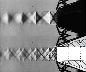
The images obtained for the ‘schlieren on’ GA solution can now be examined to further understand the potential mechanisms leveraged by the GA. An average schlieren image from 100 image samples is presented in figure 6 for the unactuated baseline case and the  $\{0,6,12,6\}$ solution obtained by the GA. The baseline image in figure 6(a) corresponds to a typical overexpanded jet, at
  $NPR=2.80$, presenting a repeating shock diamond train pattern that shows sharp interactions at the jet shear layers. The
  $\{0,6,12,6\}$ solution mean schlieren image in figure 6(b), on the other hand, shows a highly complex structure of shock cells, resulting from the addition of new bow shocks inside of the diverging section of the nozzle due to the presence of the actuators. Inside the diverging section of the nozzle, the microjets act as jets in supersonic cross-flow (Knast Reference Knast2020). The small bow shocks in front of the microjets disrupt the formation of a strongly defined shock cell structure such as the baseline case of figure 6(a). Note the disruption is so significant that the Mach disk present in the baseline case of figure 6(a) is not evident in the actuated case of figure 6(b), suggesting it was greatly weakened.

Figure 6. Mean schlieren images (vertical cutoff) of the (a) baseline and (b) GA solution obtained in § 4.1, plotted in the same colour scale. Scaled nozzle drawing overlaid to clarify actuator locations. Vertical schlieren cutoff used to acquire images.
In this sense, the extra shocks introduced by the microjets are expected to have two effects. On one hand, additional shocks originating from within the nozzle interact with the jet shear layer, increasing the minimum wavenumber  $k_1$ of the waveguide modes according to the model proposed by Tam (Reference Tam1995), which would be expected to increase the frequencies related to the BBSAN produced by the jet. On the other hand, the magnitude of the BBSAN sources may be greatly diminished if the shocks are spread out in space such that the velocity jumps across each shock are smaller in magnitude, which may explain the significant reduction in
  $OASPL$ accomplished by the GA solution. A similar effect was observed by Morris et al. (Reference Morris, McLaughlin and Kuo2013) by also actuating at the diverging section of the C–D nozzle, being highly effective in reducing noise.
The presence of the microjets blowing at the shear layer also disrupts the feedback loop mechanism responsible for screech, similar to what is observed by Alvi et al. (Reference Alvi, Lou, Shih and Kumar2008). This is readily observed in the standard deviation of the schlieren images, shown in figure 7. The unactuated case of figure 7(a), which produces screech tones at 5.7 kHz and 11.5 kHz, presents periodically spaced regions of high standard deviation outside of the jet shear layer, indicated in (a1). This structure is similar to what is observed by Edgington-Mitchell (Reference Edgington-Mitchell2019) and referred to as a standing wave pattern, characterizing the screech of the baseline jet. As the jet is actuated, as shown in figure 7(b), the standing wave pattern vanishes and the screech tone is eliminated from the spectrum, as will be further discussed in § 4.4, indicating the effectiveness of the control mechanism to eliminate jet screech.

Figure 7. Standard deviation of the schlieren images for the (a) baseline and (b) GA solution obtained in § 4.1, plotted in the same colour scale.
Lastly, it can be noted that the addition of microjets is also observed to increase the shear layer growth close to the first two shock cells in figure 7, although the growth rate seems to be lower in the most downstream portions of the jet. This effect has also been observed by Alvi et al. (Reference Alvi, Lou, Shih and Kumar2008). The effect is also evident in figure 6, where the supersonic (shock cell containing) portion of the jet core is extended farther downstream – possibly due to the reduced mixing resultant from a lower shear layer growth rate.
4.3. Evolution process – anechoic
The success obtained by the GA described in § 4.1 was highly encouraging, but the fact the GA targeted the minimization of noise as measured by the microphone behind the schlieren mirror raised questions about the generality of the solution achieved. Thus, a second GA experiment was performed after removing the schlieren optics and reinstalling all acoustic wedges back into the anechoic chamber, restoring the fully anechoic state of the chamber.
During the second GA run, 25 generations of 30 individuals were considered for a total of 750 configurations tested. The summary of the GA evolution is presented in figure 8. Once again, the GA quickly sought to minimize the sideline noise ( $\phi =90^\circ$), as the largest
  $\Delta OASPL$ indeed occurred at that angle. Thus, once again the evolution plot of figure 8(a) shows the evolution of
  $OASPL$ at the
  $\phi =90^\circ$ microphone. Convergence was slower during the second run, reaching a converged state approximately by Generation 15. However, note that the optimal actuator pattern for the second run, shown in figure 8(c), is different than the optimal actuator pattern in the previous run figure 4(c). In this second experiment, the pattern
  $\{0,0,13,12\}$ was reached as the optimal pattern. As the maximum number of actuators was 25, this pattern used all actuators made available for the GA. The actuator pressures shown in figure 8(b), were approximately the same in the optimal case as the previous solution, and the
  $OASPL$ dependence on
  $SPR3$ and
  $SPR4$ is very similar to what is previously shown for the ‘schlieren on’ experiment in figure 5, with an asymptotic behaviour about
  $SPR\sim 1.7$. The pressure for EPR1 and EPR2 are not shown in figure 8(b) as they had no active actuators in most of the best cases on each generation.

Figure 8. Results from the second GA experiment without a schlieren (fully anechoic). (a) Evolution of the  $OASPL$ captured by the microphone at
  $\phi =90^\circ$ against the baseline case. Blue band represents variability between baseline cases. (b) Setpoint of EPRs for best individual on each generation. (c) Number of active actuators for the best individual on each generation.
Once again, the actuator patterns in figure 8(c) indicate actuating at ring R1 (in the converging section of the nozzle) is highly ineffective. In fact, plotting the measured  $OASPL$ at
  $\phi =90^\circ$ against the mass flow rate at the ring R1 (
 $\dot {m}_{R1}$) for all the cases explored in the anechoic GA run reveals an interesting pattern, shown in figure 9(a). The mass flow rate was measured by an Omega FMA5410 mass flow meter with the main nozzle inactive for all actuators as a function of the pressure at the EPR, and a quadratic curve fit based on these measurements is used to estimate the mass flow rate during the experiment. The main nozzle mass flow rate (
 $\dot {m}_{Nozzle}=336.5\ {\rm g}\ {\rm s}^{-1}$) is estimated from the 1-D isentropic relations for the overexpanded
  $NPR=2.80$. Figure 9(a) shows that as the mass flow rate in the ring R1 is increased (i.e. increasing number of active actuators and the corresponding
  $SPR$), the minimum
  $OASPL$ attained by the GA increases. This would suggest that actuating at the converging section of the nozzle is not only ineffective, but potentially detrimental to the goal of noise reduction. This effect is further evidenced by a measurement performed for the
  $\{16,0,0,0\}$ configuration (i.e. only a full R1 ring) at a mass flow ratio of
  $\dot {m}_{R1}/\dot {m}_{Nozzle}=0.7\,\%$, which yielded a small increase in
  $OASPL$ at the
  $\phi =90^\circ$ microphone of 1.1 dB. At the position where the actuators R1 are located, the local cross-sectional area of the nozzle channel is 1.043 times the throat area, meaning the local Mach number is approximately 0.96. Thus, actuating at R1 may significantly change the boundary layer and flow conditions at the throat, as well as the effective throat area. Unfortunately, the data gathered in this experiment is not sufficient to specify how such changes to the throat conditions would increase the noise produced by the main jet.

Figure 9. Effect of mass flow rate at (a) ring R1 and (b) all rings on the  $OASPL$ for the fully anechoic GA experiment.
As presented in figure 9(b), the total mass flow rate used by all actuators is always maintained under  $\dot {m}_{Total}/\dot {m}_{Nozzle}<1.7\,\%$. The same general trend previously observed in figure 5 is also observed in figure 9(b), that is, increasing the actuator mass flow rate has a generally beneficial effect to noise reduction up until a threshold value (
 $\dot {m}_{Total}/\dot {m}_{Nozzle} \sim 1\,\%$), and further increases in mass flow rate then have little effect on
  $OASPL$ within the range observed. For the optimal configuration with most noise reduction,
  $\dot {m}_{Total}/\dot {m}_{Nozzle} = 1.4\,\%$ and
  $J=\max (\Delta OASPL_m)=7.3$ dB.
4.4. Far field acoustics
In this section, a more detailed analysis of the acoustics of the different cases explored will be presented. All acoustical data presented in the following sections consists of measurements performed in the fully anechoic configuration, with 10 s-long data sets for improved statistical convergence.
The directivity of the jet noise captured by the microphone array is presented in figure 10(a), comparing the baseline unactuated case with the two GA solutions obtained in the experiments described in §§ 4.1 and 4.3. The difference between the baseline  $OASPL$ and the
  $OASPL$ of the anechoic GA solution
  $\{0,0,13,12\}$ is annotated in figure 10(a) in red. Note the largest
  $\Delta OASPL$ occurs at the sideline
  $\phi =90^\circ$ noise, which is plotted over time in figure 10(b) together with the baseline case to show the drastic difference in waveform amplitude as the actuators are toggled. A significant reduction is observed in all radiation directions, ranging from
  $-3.3$ dB to
  $-7.3$ dB, which is an accomplishment considering the approach used is model-free. The more upstream microphones, closer to the sideline
  $\phi =90^\circ$ direction, observed the largest noise reductions. This is a similar behaviour to what was observed in a recent study (Liu et al. Reference Liu, Khine, Saleem, Rodriguez and Gutmark2022) on a faceted C–D nozzle, which reports the application of 12 microvortex generators at the diverging walls of the nozzle, also observing noise reduction of 5–6 dB at the sideline and upstream directions. Thus, introducing small disturbances at the diverging section is a reasonable strategy for supersonic jet noise reduction in the sideline and upstream directions, which was effectively leveraged by the GA. Both GA solutions have approximately the same effect on the overall noise, however, the
  $\{0,0,13,12\}$ solution is slightly more effective (
 $\sim$0.5 dB) at reducing jet noise than the
  $\{0,6,12,6\}$ beyond the (
 $\pm$0.02 dB) uncertainty on the statistical convergence of
  $OASPL$. Considering the solutions were attained in two different runs of the GA with different random seeds, it is reasonable to say they are equivalent solutions, at least from the perspective of the goal function
  $J$ defined.

Figure 10. (a) Effect of the actuation schemes found by the GA on jet noise directivity. Red numbers represent  $\Delta OASPL$ for the
  $\{0,0,13,12\}$ solution. All cases evaluated in anechoic conditions. (b) Time series of the
  $\phi =90^\circ$ microphone as the
  $\{0,0,13,12\}$ actuators are toggled.
Closer examination of figure 10(b) indicates that the baseline time traces are positively skewed ( ${\rm skewness} = 0.22$), even though their mean is zero. The skewness is removed in the actuated case. As noted by Greska, Krothapalli & Arakeri (Reference Greska, Krothapalli and Arakeri2003) and Krothapalli, Venkatakrishnan & Lourenco (Reference Krothapalli, Venkatakrishnan and Lourenco2000), the skewness is attributed to crackle events, which are sudden, large deviations from the mean over short time scales. The use of microjets in the GA solution, similarly to what was found in Greska et al. (Reference Greska, Krothapalli and Arakeri2003), eliminates this effect, which may also contribute to a significant fraction of the noise reduction observed.
A closer look at the spectral content captured by the microphones at selected angles is provided in figure 11 in both physical and normalized frequencies, obtained through the averaged periodogram method (Welch Reference Welch1967) with 4096 averages. The Strouhal frequencies ( $St_{D_e}=f D_e/U_e$) are normalized by the exit diameter
  $D_e=27.55$ mm and exit velocity
  $U_e=431\ {\rm m}\ {\rm s}^{-1}$, estimated through isentropic relations. As is typical, the more downstream angles
  $\phi =30^\circ$ and
  $\phi =45^\circ$ in figure 11(a,b) contain higher energy at lower frequencies
  $St_{D_e}\sim 0.2$, which are related to turbulent mixing noise and are broadband in nature. At these angles, the noise reduction promoted by the GA actuation schemes is lower but is consistent across most frequencies in the spectrum. At very low frequencies (
 $St_{D_e}< 0.08$), however, the GA solutions are mostly ineffective at reducing very large-scale mixing noise. Noting that this very low frequency part of the spectrum (
 $St_{D_e}< 0.08$) contains a very small fraction of the total noise energy in the baseline case (0.25 % for
  $\phi =90^\circ$ and 3.7 % for
  $\phi =30^\circ$), it was not prioritized during the optimization in face of significantly larger noise sources, such as the screech tone and the BBSAN.

Figure 11. Effect of GA-based actuation on the noise spectra at different polar directions.
At the two more upstream angles  $\phi =60^\circ$ and
  $\phi =90^\circ$ in figure 11(c,d), a greater reduction in noise is observed at all frequencies. Evidently, this reduction across the entire spectrum culminates in the larger reduction in
  $OASPL$ at these locations. Also important to note is the disappearance of the screech tones at
  $St_{D_e}= 0.364$ and
  $St_{D_e}=0.735$, which agrees with the disappearance of the standing wave observed in the schlieren standard deviation images of figure 7. Note that the energy contained in the screech tones of the baseline case at
  $\phi =90^\circ$ was 37 % of the total power contained in the spectrum, meaning the elimination of the screech tone would contribute to a
  $-10\log _{10} (1-0.37)=2.03$ dB reduction in
  $OASPL$. Thus, although the overall spectrum experiences a reduction in
  $OASPL$, a portion of the reduction in noise is due to the elimination of the screech tone.
A spectral hump is observed at  $\phi =90^\circ$ in both baseline and actuated cases, peaking at
  $St_{D_e}\sim 0.85$ and
  $St_{D_e}\sim 1.1$, respectively. This high-frequency broadband peak is typically associated with the BBSAN. In the baseline case, the broadband peak occurs around
  $f\sim 12.3$ kHz, matching the predicted BBSAN peak by the early model of Harper-Bourne & Fisher (Reference Harper-Bourne and Fisher1977), considering the measured shock cell spacing of 25.7 mm (figure 6). In the baseline case at
  $\phi =90^\circ$, 59.4 % of the total noise energy is contained within the high (
 $f>8$ kHz) frequency range, excluding the screech tone peak, indicating the BBSAN is also a noise source worthwhile targeting during the noise optimization process. In the
  $\{0,0,13,12\}$ solution, the energy in this high-frequency (
 $f>8$ kHz) range is reduced to 28 % of the baseline value, demonstrating how the GA successfully targeted the BBSAN mechanism to effectively reduce the noise produced by the main jet.
Furthermore, the fact the actuated cases shift the peak frequency of the BBSAN to a higher frequency is further evidence that the mechanism proposed in § 4.2 (i.e. that the extra shocks produced by the microjets increase the wavenumbers of the waveguide modes) plays a role in the shaping of the acoustic spectrum. However, since the shock cell spacings are uneven, it is unclear whether the simple model by Harper-Bourne & Fisher (Reference Harper-Bourne and Fisher1977) still applies. The effectiveness of this actuation scheme on targeting the BBSAN also explains why the GA targeted the  $\phi =90^\circ$ microphone during the optimization process, as it was the most readily available mechanism to be leveraged using the microjet locations provided. Utilizing a more downstream location, such as the
  $\phi =30^\circ$ microphone, for the definition of the goal function may have yielded a solution with more focus on noise reduction at the lower frequencies associated with turbulent mixing.
Also worth discussion is the strong similarity of the spectra between the two GA solutions (red and blue curves in figure 11), as well as the  $OASPL$ values in figure 10(a). This similarity would suggest the two actuation schemes, although activating different rings, are accomplishing a very similar overall result in the acoustic field. Further examination of the GA evolution process in the ‘schlieren on’ phase of this experiment indicate that ring R2 may not have been a key contributor to the GA solution. Through the ‘teleport ring’ function in the GA mutation procedure, two rings can be swapped, generating alternative configurations that can be examined. Remembering that the optimal
  $\Delta OASPL=8.6$ dB for the
  $\{0,6,12,6\}$ solution in the ‘schlieren on’ configuration at
  $\phi =90^\circ$, alternative configurations with similar EPR values are found at
  $\{12,6,0,6\}$ (
 $\Delta OASPL=4.4$ dB), and
  $\{6,0,12,6\}$ (
 $\Delta OASPL=7.6$ dB). Note the former configuration swaps rings R1 and R3, moving the actuators of R3 to a less effective location (R1), yielding significant performance drop on the
  $\Delta OASPL$ and indicating the 12 actuators on ring R3 are essential to the solution. Conversely, swapping rings R1 and R2 (i.e. configuration
  $\{6,0,12,6\}$) does not yield a significant performance drop, indicating ring R2 is not as essential to the solution as ring R3 and potentially its presence was a limiting factor on the evolution of the GA in the ‘schlieren on’ experiment, as the maximum number of actuators was limited to 25. Under the light of this observation, one could conclude the ‘anechoic’ GA solution may be slightly more optimal, as it maximizes the available number of actuators at the rings that are most effective (i.e. rings R3 and R4).
An examination of the cases where actuation is provided as a full ring of actuators at ring R3 ( $\{0,0,16,0\}$) and ring R4 (
 $\{0,0,0,16\}$) at a corresponding
  $SPR=1.7$ can be useful to isolate the effects of the two rings in the ‘anechoic’ GA solution
  $\{0,0,13,12\}$. The
  $\phi =90^\circ$ spectra of the single-ring actuation schemes are presented in figure 12(a) in solid magenta and green lines, accompanied by the spectra of the previously discussed GA solutions as dashed lines. It is immediately noticed that the actuation only at ring R3 (magenta line) does not eliminate the screech tone, also slightly lowering its frequency as well as the BBSAN hump peak frequency. The overall levels of the BBSAN hump, however, are significantly lowered in the full R3 case, indicating the addition of new, weaker shock cells positively contributes to broadband shock noise reduction. A lengthening of the first shock cell is also observed when comparing the shadowgraphs of figures 12(b) and 12(c), which is consistent with the lowering of the peak frequencies in the spectrum. Conversely, actuating only ring R4 (green line in figure 12a) increases the BBSAN hump peak frequency, eliminates the screech tone and reduces the length of the first shock cell, as can be noted in figure 12(d). Thus, it appears that actuating the shear layer of the jet is responsible for disrupting the feedback loop that causes the jet to screech, also having a smaller effect on the reduction of the BBSAN noise amplitude. The effects of rings R3 and R4 compound on the GA solution found in anechoic conditions
  $\{0,0,13,12\}$, resulting in significant reduction of BBSAN as well as the elimination of the screech tone.

Figure 12. (a) Comparison of the spectra of the GA-based actuation schemes with the single full ring actuation at  $\phi =90^\circ$,
  $SPR=1.7$. All spectra captured at anechoic conditions. (b–d) Shadowgraphs of the first two shock cells for the baseline and full ring cases.
4.5. Effect of $NPR$

Utilizing the optimal GA-based actuator scheme yielded 7.3 dB  $OASPL$ reduction at the most effective direction (
 $\phi =90^\circ$). A follow-up question is how effective this actuation scheme would be at different operational conditions of the main jet. In this section, the effect of
  $NPR$ will be examined for the baseline and the
  $\{0,0,13,12\}$ solution obtained in the anechoic GA experiment. The results herein noted also apply very closely to the
  $\{0,6,12,6\}$ solution, which was also tested for
  $NPR$ effects but is omitted for clarity of the discussion. Thrust, including potential losses, could not be estimated in the present study as it was designed to focus on acoustics.
For this experiment, a parametric scan of  $NPR$ was performed by sequentially opening the main jet control valve and acquiring data for 10 s, while maintaining the remaining conditions fixed (i.e. one scan for the baseline case and another for the actuated case). Between
  $2.7< NPR<2.9$, an increased number of points was taken to ensure repeatability of the results previously described. The parameter scan is summarized in figure 13 by showing the
  $OASPL$ measured by selected microphones as a function of
  $NPR$ for both baseline and GA solution cases. The difference between the cases (
 $\Delta OASPL$) was computed by linearly interpolating the baseline/actuated data sets prior to computing the difference, as the
  $NPRa$ of each data set were slightly mismatched. The mismatch did not exceed
  $\Delta NPR=0.02$ in any case considered.

Figure 13. Effect of  $NPR$ on the
  $OASPL$ produced by the jet at different polar directions.
Figure 13(d) shows that the peak noise reduction occurred, serendipitously, very close to the  $NPR=2.80$ chosen for the experiment. More specifically, the peak reduction of 7.9 dB at
  $\phi =90^\circ$ occurred at
  $NPR=2.73$. As is typically observed in C–D nozzles, the sideline noise trend for the baseline case has an ‘N’ shape, with the noise levels increasing for the overexpanded jet and then decreasing as the nozzle approaches ideally expanded conditions, where a local noise minimum occurs as the strength of the shocks is minimized. The
  $NPR$ where this minimum occurs in this experiment is
  $NPR=3.45\pm 0.15$, which is slightly different from the design
  $NPR_d=3.69$. Increasing pressure past this
  $NPR$ then monotonically increases the noise levels. Actuating the nozzle with the GA
  $\{0,0,13,12\}$ solution changes this ‘N’ curve into a simple monotonic increase in
  $OASPL$ as a function of
  $NPR$, which is observed in all polar directions. At the downstream directions
  $\phi =30^\circ$ and
  $\phi =45^\circ$ the actuated cases always reduce noise, even close to ideally expanded
  $NPR$ values, as is shown in figure 13(a,b). Note in this experiment that the
  $SPR$ of the microjet actuators is not being increased, meaning the ratio of actuator mass flow with respect to the main nozzle is greatly decreasing as the
  $NPR$ is increased.
Conversely, a crossover behaviour can be observed in the more upstream microphones  $\phi =60^\circ$ and
  $\phi =90^\circ$. As the
  $NPR$ is increased towards ideally expanded conditions, the actuation becomes less effective and then becomes detrimental to noise reduction between
  $3.35< NPR<3.9$, increasing the noise produced by up to 2.1 dB in the worst case at
  $\phi =90^\circ$ and
  $NPR=3.45$. This stands to reason as the microjets always induce a bow shock that will lead to a shock train within the jet, which by itself is an important source of noise. When the baseline case does not produce strong shocks, as is the case close to ideally expanded conditions, then actuating adds undesirable noise sources. At underexpanded conditions, the benefit of actuating becomes significantly lower, only reaching 0.5 dB noise reduction at the highest
  $NPR$ considered of 4.1. As the actuator experimental set-up would need increased supply pressures to maintain similar mass flow ratios or similar momentum coefficients, it is possible that significantly better noise reduction could be achieved with the same actuator distribution found by the GA. The mass flow ratio is estimated to be
  $\dot {m}_{Total}/\dot {m}_{Nozzle} = 0.9\,\%$ at the most underexpanded case (
 $NPR=4.1$). It is likely that different optimal configurations of microjet actuators exist for the underexpanded and ideally expanded cases, which would require a dedicated optimization experiment.
The observed trends in  $OASPL$ as a function of
  $NPR$ for the baseline and actuated cases are more readily understood by analysing the spectral content of the corresponding cases. Spectra for representative
  $NPR$ values are presented in figure 14. Note in all cases the low-frequency turbulent mixing noise is slightly reduced, and this reduction is more pronounced around
  $NPR=3.0$ as shown in figure 14(b). Also, in all cases the frequency of the BBSAN-associated hump is increased, which is noted in figure 14 by the grey arrows. The case
  $NPR=3.45$, displayed in figure 14(c) and selected because its baseline
  $OASPL$ was the lowest in the parameter scan, has a negligible BBSAN content and is likely the closest this real nozzle is to ideally expanded conditions. Evidently, the addition of actuators that introduce shocks introduces a BBSAN-related hump in the spectrum, which is clearly seen as a hump that peaks around 25 kHz. This effect can readily be observed in the long-exposure (10 ms) schlieren photographs of figure 15, which were also captured at the design
  $NPR$ of this nozzle (3.67), although for the ‘schlieren on’ GA solution
  $\{0,6,12,6\}$. The introduction of microjets introduces shocks that enable the production of BBSAN that were absent in the unactuated jet. Note this additional noise source is solely responsible for the 2.1 dB increase in
  $OASPL$ noise levels in the
  $NPR=3.45$ case, as the remainder of the spectral content (i.e. at frequencies lower than 15 kHz) is lower in energy than the baseline.

Figure 14. Effect of  $NPR$ on the spectra of the
  $\phi =90^\circ$ microphone for the baseline and actuated cases. Grey arrows indicate BBSAN peak frequency shift.

Figure 15. Schlieren images (horizontal cutoff) of (a) unactuated and (b)  $\{0,6,12,6\}$ actuation at
  $NPR=3.67$.
At underexpanded conditions ( $NPR=4.1$, figure 14d), an appreciable reduction in the BBSAN hump is also observed. Although not investigated herein, it is possible further improvement may be possible through increased actuation mass flow rate. Finally, at highly overexpanded conditions (
 $NPR=2.4$, figure 14a), the addition of the microjets resulted in an overall reduction in noise (
 $\Delta OASPL=1.4$ dB) by elimination of the screech tone and reduction in turbulent mixing noise, but the actuator mass flow rate may have been excessive, as the BBSAN levels increased. A parametric scan on the mass flow rate parameter was not performed at this time, but it is reasonable to assume that if the BBSAN noise reduction mechanism is related to the spreading of the shock train there would be an optimal point beyond which additional actuator power would produce bow shocks that are stronger than the original baseline shock, resulting in an increased production of noise.
4.6. Effect of temperature
An experiment at a higher stagnation temperature of  $T_0=560\pm 3$ K and
  $NPR=2.80\pm 0.04$ was performed to understand the effect of temperature on the effectiveness of the actuator schemes found by the GA for a cold jet as described in the previous sections. The cases with
  $T_0=560$ K will be considered ‘hot’ cases through this section, at a nozzle temperature ratio of
  $NTR=1.88$, although the stagnation temperature is not as high as is typical in supersonic engines. All cases are measured under fully anechoic conditions. As the actuator assembly materials were not appropriate to run for extended periods of time under the ‘hot’ conditions, the experiments were limited to 5 min, which prevented the deployment of the GA in this part of the study.
The effect of temperature on the noise directivity is presented in figure 16 for both actuation schemes found by the GA. Comparing the red and black lines from the respective hot and cold baseline cases, a general increase in  $OASPL$ is observed in all directions, with the largest increase at the most downstream microphone (
 $\phi =30^\circ$). At the sideline microphone, a marginal increase in
  $OASPL$ of
  $0.4$ dB is observed as the baseline jet temperature is increased. Utilizing the actuation schemes encountered by the
  $GA$ is not as effective in the hot cases, however. A maximum reduction of 4.7 dB in
  $OASPL$ at the sideline microphone
  $\phi =90^\circ$ is observed, which is much lower than the 7.3 dB reduction observed for the cold jet. Once again, both actuation schemes perform similarly in the hot case, but the {0,0,13,12} pattern is slightly more effective by
  ${\sim }0.5$ dB. A lower degradation in actuator effectiveness for the hot case is observed at the downstream stations (
 $\phi <60^\circ$), with similar
  $\Delta OASPL$ results when compared with the cold case of figure 10.

Figure 16. Effect of the temperature jet noise directivity for baseline and GA actuated cases. Magenta numbers represent  $\Delta OASPL$ for the
  $\{0,0,13,12\}$ solution.
To understand the reduced effectiveness of the actuation schemes, a closer look at the spectra of microphones at two different polar angles is presented in figure 17. Both microphones at figure 17(a,b) detect an overall increase in low-frequency turbulent mixing noise for the baseline hot case, when compared with the baseline cold case. At  $\phi =30^\circ$, in figure 17(a), the mixing noise increases in amplitude at the higher frequencies, which explains the greatly increased
  $OASPL$ at this directivity angle. Additionally, the screech tone now radiates towards the
  $\phi =30^\circ$ microphone, presenting a peak at 6.3 kHz and contributing to the increased noise levels. At
  $\phi =90^\circ$, in figure 17(b), an increase in the low-frequency mixing noise is observed for the baseline hot case, but the higher frequency BBSAN remains approximately constant. The screech tone slightly drops in amplitude, resulting in a negligible increase in
  $OASPL$ at this radiation angle.

Figure 17. Comparison between the spectra of the baseline and actuated cases at two stagnation temperatures.
Comparing the magenta (actuated, hot) and red (baseline, hot) lines in figure 17(b), a significant reduction of  $SPL$ through the spectrum can still be observed. However, the drop in
  $SPL$ is lower in magnitude and does not occur for ultrasonic frequencies (
 $f>20$ kHz). The screech tones are, once again, eliminated in the actuated case. The BBSAN-related hump is also shifted to significantly higher frequencies, but the lack of effect at the ultrasonic frequencies seems to be responsible for the overall performance degradation observed in figure 16.
As the ‘anechoic’ GA solution  $\{0,0,13,12\}$ utilized all 25 available solenoids during the optimization experiment, it was conjectured that using all available actuators in the two downstream rings (R3, R4) would probably be the optimal solution if that constraint was not enforced. Thus, prior to running the hot experiments, a few checks and modifications to the solenoid power supply were performed to enable the usage of two full rings (32 actuators) for a limited amount of time. The directivity plot for the full (R3, R4) rings under hot conditions is compared with the GA solution in figure 18(a). Curiously, using the full (R3, R4) rings (
 $\{0,0,16,16\}$ in figure 18a) leads to a change in the directivity characteristics of the actuated jet. On one hand, the
  $\{0,0,16,16\}$ solution causes further reduction in
  $OASPL$ at the downstream
  $\phi =30^\circ$ microphone (4.4 dB reduction instead of 3.9 dB reduction). On the other hand, the sideline
  $\phi =90^\circ$ microphone observes an increase in
  $OASPL$ when compared with the
  $\{0,0,13,12\}$ solution (3.6 dB reduction instead of 4.7 dB reduction). Thus, from the
  $J$ fitness function perspective, the GA solution is indeed better, as there is a directivity trade-off between rings R3 and R4.

Figure 18. Directivity comparison of the  $\{0,0,13,12\}$ GA solution with manually selected actuator configurations utilizing full rings. All cases evaluated under high temperature (
 $T_0=560$ K).
As observed by Castelain et al. (Reference Castelain, Sunyach, Juvé and Béra2008), a corrugation of the shear layer on the main jet occurs due to the microjets impinging on it, corresponding to ring R4 in the current experiment. This shear layer corrugation was observed to be correlated to a  $\sim$1 dB reduction of turbulent mixing noise for a
  $M=0.9$ jet. In the current experiment, increasing the number of jets on ring R4 from 12 (
 $\{0,0,13,12\}$ in figure 18a) to 16 (
 $\{0,0,16,16\}$ in figure 18a) provides a further 0.5 dB noise reduction at the downstream
  $\phi =30^\circ$ microphone, which would suggest this shear layer corrugation effect may be responsible for a portion of the turbulent mixing noise reduction.
The effect of the individual rings R3 and R4 was also investigated at this stage of the experimental campaign. A plot of directivity for the individual, but fully actuated rings R3 and R4 is presented in figure 18(b) and compared with the baseline and GA solution  $\{0,0,13,12\}$ cases. Note that each individual ring causes a reduction in
  $OASPL$ at all directivity angles, however, the reduction in
  $OASPL$ obtained by the GA solution
  $\{0,0,13,12\}$ cannot be fully explained by only one of the rings. In past literature studies (Greska & Krothapalli Reference Greska and Krothapalli2005; Castelain et al. Reference Castelain, Sunyach, Juvé and Béra2008; Zaman Reference Zaman2010), it was very common to use actuation at a ring externally mounted to the nozzle (like ring R4), which presents operational advantages such as interchangeability between nozzles. However, actuating ring R4 is not optimal, yielding only 2.1 dB
  $OASPL$ reduction at the sideline
  $\phi =90^\circ$ direction as can be noted in figure 18(b), which is comparable to the results found by Castelain et al. (Reference Castelain, Sunyach, Juvé and Béra2008). Actuating inside the nozzle diverging section, at ring R3, is significantly more effective, yielding 3.5 dB reduction at the sideline direction. Ring R3 is not as effective in the downstream
  $\phi =30^\circ$ direction, however, yielding only 0.7 dB
  $OASPL$ reduction in that microphone. Thus, it is a combination of the two rings, such as the GA solution
  $\{0,0,13,12\}$ case, which yields maximum
  $OASPL$ reduction across all directivity angles.
The reduced effectiveness of the individual rings R3 and R4 can be broken down when analysing the spectra presented in figure 19, which is shown for  $\phi =90^\circ$. Ring R3 (black line) has an appreciable impact in low frequency turbulent mixing noise, as well as in the high-frequency BBSAN region. However, actuating ring R3 does not eliminate the screech tones, although it does reduce their amplitude (
 $\sim$7.5 dB). Conversely, actuating externally to the nozzle (ring R4, blue line in figure 19) is very effective in reducing low frequency turbulent mixing noise, which further supports the shear layer corrugation effect observed by Castelain et al. (Reference Castelain, Sunyach, Juvé and Béra2008) is related to large scale mixing noise reduction. Furthermore, actuating ring R4 also eliminates the screech tone, but increases the high-frequency BBSAN above the baseline level, which leads to poor
  $OASPL$ reduction. By actuating both rings with the optimal number of actuators, the GA found this compromise between screech, turbulent mixing noise and BBSAN that is by no means straightforward, reaching the significant reductions in noise levels observed in this study.

Figure 19. Comparison between the spectra of baseline and individual ring (R3 or R4) cases, measured at  $\phi =90^\circ$. All cases evaluated under high temperature (
 $T_0=560$ K).
Finally, it is worth noting that a GA optimization was not performed with the heated jet in this study. However, it is evident in figure 16 that the noise levels are significantly increased at the  $\phi =30^\circ$ direction, reaching 127.4 dB. The
  $OASPL$ at
  $\phi =30^\circ$ is thus 10.5 dB higher than at the sideline
  $\phi =90^\circ$ direction, meaning it poses a greater risk of hearing damage if one considers an aircraft carrier application where noise from heated supersonic jets is of interest. Thus, from an application perspective, it may be more appropriate to define
  $J$ as a cost function that considers the worst-case noise direction (e.g. minimize
  $J=\max [OASPL_{actuated,m}]$).
5. Conclusion
In this study, a novel experimental test bench is developed to minimize the noise produced by an overexpanded, circular supersonic nozzle by using active flow control, leveraging an automated genetic algorithm-based optimization procedure that does not require prior knowledge of the flow physics to tackle the noise reduction problem. An  $OASPL$ reduction of 7.3 dB in sideline noise is observed in the cold jet case at
  $NPR=2.8$, and the same actuation scheme was tested at a higher stagnation temperature (560 K), yielding 4.7 dB
  $OASPL$ reduction. The reductions in noise in both cases are significant and readily noticeable. The approach herein described is compelling in that hundreds of actuator configurations are deployed in a single experiment, encompassing a large subset of the configurations that are possible to build given the limitations of the experimental apparatus.
Closer examination of the flow properties through flow visualization and analysis of the spectra of the different cases tested led to a few interesting lessons for future control efforts under similar conditions: (1) actuating on the diverging walls of the nozzle is highly effective at reducing the BBSAN and turbulent mixing noise, but not as effective at reducing the screech tone; (2) actuating outside of the nozzle, just downstream of the lip, is effective in eliminating screech but increases the BBSAN, leading to poor overall performance; (3) thus, a combined approach using both external and internal actuation at the diverging wall is optimal, as was detected by the GA; (4) actuating at the diverging wall introduces bow shocks at the microjet locations, which disrupts the structure of the shock cell train produced by the overexpanded jet, weakening the individual shocks and potentially contributing to the reduction in BBSAN; (5) the disruption of the periodic shock cell structure changes the supported waveguide modes, shifting the BBSAN peak to higher frequencies; and (6) actuating at the converging section of the C–D nozzle is not effective at reducing noise, potentially being detrimental to the performance of other noise reduction schemes.
The solution encountered by the GA was then tested at  $NPR$ values outside of the conditions used for optimization, to understand the effect of jet expansion in the actuator effectiveness. It was found that there is an
  $NPR$ range where the GA actuation scheme increases noise, coinciding with the region where the baseline jet noise is closest to a local minimum. At the nominally ideally expanded case, the schlieren image and microphone spectra show evidence that the microjet actuators introduce shocks in an otherwise shock-free flow (or a flow containing weak shocks). Thus, the observed noise increase due to actuation stems from the increase in BBSAN due to the introduction of new shocks. Finally, at underexpanded
  $NPRs$ the actuation scheme was also effective in reducing noise, however, to a lesser extent – possibly due to the relatively lower momentum coefficient of the microjet actuators, which were limited in pressure by the experimental set-up.
Funding
The authors would like to thank the Office of Naval Research (ONR) and the Air Force Office for Scientific Research (AFOSR) for the financial support provided for the development of this work.
Declaration of interests
The authors report no conflict of interest.


