


1. Introduction
Turbulent convection is the key mixing and transport process in many natural environments, and understanding the heat flux and the turbulence level in such flows is of fundamental importance, especially for the circumstances where the thermal driving is extremely strong (Ahlers, Grossmann & Lohse Reference Ahlers, Grossmann and Lohse2009; Chillà & Schumacher Reference Chillà and Schumacher2012; Xia Reference Xia2013; Plumley & Julien Reference Plumley and Julien2019). The paradigmatic model for turbulent convection is the Rayleigh–Bénard (RB) flow, namely the buoyancy-driven flow within a fluid layer heated from below and cooled from above. For a given fluid with certain Prandtl number  ${Pr = \nu /\kappa}$, the thermal driving force is measured by the Rayleigh number
  $Ra = (g \alpha \Delta H^{3})/(\nu \kappa )$. Here,
  $\nu$ is kinematic viscosity,
  $\kappa$ is thermal diffusivity,
  $g$ is the gravitational acceleration,
  $\alpha$ is the thermal expansion coefficient,
  $\varDelta$ is the temperature difference across the layer and
  $H$ is the layer height, respectively. The key response of the system is the heat flux and the flow velocity. The former is usually measured by the Nusselt number
  $Nu$, i.e. the ratio between the total flux to the conductive flux, while the latter by the Reynolds number
  $Re=UH/\nu$. Here
  $U$ is some characteristic velocity, and
  $H$ usually the height of the fluid layer.
The dependences of  $Nu$ and
  $Re$ on both
  $Pr$ and
  $Ra$ have been studied extensively in the past. Usually, a power-law scaling is assumed as
  $Nu \sim Ra^{\gamma }$ and the exponent
  $\gamma$ is determined by either theoretical analysis or measurement. For instance, by a marginal-stability analysis Malkus (Reference Malkus1954) obtained
  $\gamma = 1/3$. Priestley (Reference Priestley1954) assumed that the heat flux is independent of the layer height
  $H$ due to the turbulent bulk, and arrived at the same exponent
  $\gamma =1/3$. Comprehensive reviews about the early models can be found in Ahlers et al. (Reference Ahlers, Grossmann and Lohse2009) and Chillà & Schumacher (Reference Chillà and Schumacher2012). When the boundary layers are not fully turbulent and serve as the bottleneck for heat transfer, as in the cases for weak to moderate thermal driving, one usually has an exponent
  $\gamma \leqslant 1/3$; this is referred to as the classic regime.
It was first postulated by Kraichnan (Reference Kraichnan1962) that when the thermal driving is strong enough, the flow will enter a different state, i.e. the ultimate regime. The key idea is that the boundary layers become fully turbulent, and both viscosity and diffusivity do not affect the heat flux. Then both  $Nu$ and
  $Re$ scale as
  $Ra^{1/2}$ subjected to a logarithmic correction. The resulting effective exponent
  $\gamma$ is larger than the value in the classic regime. Later, for the convection flow in astrophysical systems, Spiegel (Reference Spiegel1971) proposed a similar scaling law without the logarithmic correction, namely
  $Nu \sim Ra^{1/2}Pr^{1/2}$, where the flow is assumed to be not influenced by boundary layers. The unifying theory developed by Grossmann & Lohse (Reference Grossmann and Lohse2000, Reference Grossmann and Lohse2001, Reference Grossmann and Lohse2002, Reference Grossmann and Lohse2004), which successfully describes most of the existing experimental and numerical data, predicts that for the ultimate regime the following scaling laws hold:
 \begin{equation} Nu \sim Pr^{1/2} Ra^{1/2}, \quad Re \sim Pr^{{-}1/2} Ra^{1/2}. \end{equation}
All of the above models predict  $Nu$ many orders of magnitude larger than the classic scaling at very large
  $Ra$ as in various natural environments.
Tremendous efforts have been made to achieve the ultimate scaling in RB flow by both experiments and simulations at very large  $Ra$ (Chavanne et al. Reference Chavanne, Chillà, Castaing, Hebral, Chabaud and Chaussy1997; Glazier et al. Reference Glazier, Segawa, Naert and Sano1999; Niemela et al. Reference Niemela, Skrbek, Sreenivasan and Donnelly2000; Stevens et al. Reference Stevens, Lohse and Verzicco2011; He et al. Reference He, Funfschilling, Nobach, Bodenschatz and Ahlers2012; Zhu et al. Reference Zhu, Mathai, Stevens, Verzicco and Lohse2018; Iyer et al. Reference Iyer, Scheel, Schumacher and Sreenivasan2020). Some of them reported evidences of the transition to the ultimate regime (Chavanne et al. Reference Chavanne, Chillà, Castaing, Hebral, Chabaud and Chaussy1997; He et al. Reference He, Funfschilling, Nobach, Bodenschatz and Ahlers2012; Zhu et al. Reference Zhu, Stevens, Verzicco and Lohse2017, Reference Zhu, Mathai, Stevens, Verzicco and Lohse2018), while others did not. Alternative methods were used to trigger an early transition to the ultimate regime. For instance, wall roughness was introduced to generate extra perturbation to the boundary layer and therefore alter the scaling behaviour. Indeed Xie & Xia (Reference Xie and Xia2017) found that when the thickness of the thermal boundary layer is smaller than the roughness height, the scaling exponent is greatly enhanced. A closer investigation revealed that the increase of the scaling exponent is probably due to the fact that the tips of roughness are higher than the thermal boundary layer and directly transfer heat into the bulk (Salort et al. Reference Salort, Liot, Rusaouen, Seychelles, Tisserand, Creyssels, Castaing and Chillà2014). However, it was shown that for a given roughness, when
  $Ra$ is large enough, the boundary layers become very thin and follow the irregular surface. Then the scaling exponent
  $\gamma$ reduces to the value of classic scaling (Zhu et al. Reference Zhu, Stevens, Verzicco and Lohse2017, Reference Zhu, Stevens, Shishkina, Verzicco and Lohse2019). Modifications to the bulk dynamics were also employed and successfully enhanced the scaling exponent
  $\gamma$. One example is the internal heating model where a direct heating source is introduced in the bulk (Goluskin & Spiegel Reference Goluskin and Spiegel2012; Goluskin Reference Goluskin2016; Goluskin & van der Poel Reference Goluskin and van der Poel2016; Wang, Lohse & Shishkina Reference Wang, Lohse and Shishkina2021). Experiments of this type indeed show an increased scaling exponent when the radiative heating bypasses the boundary layer (Lepot, Aumaître & Gallet Reference Lepot, Aumaître and Gallet2018; Bouillaut et al. Reference Bouillaut, Lepot, Aumaître and Gallet2019). Oscillating body force was also applied to the momentum balance (Wang, Zhou & Sun Reference Wang, Zhou and Sun2020), and the scaling exponent can be increased to a value very close to that given by the ultimate scaling.
Another insightful approach is the homogeneous turbulent convection driven by background temperature gradient (Lohse & Toschi Reference Lohse and Toschi2003; Calzavarini et al. Reference Calzavarini, Lohse, Toschi and Tripiccione2005). Such a system has periodic boundary conditions in all directions and therefore removes the influence from the boundary layers, and the exponent  $\gamma$ agrees with the ultimate scaling in this ‘bulk-only’ convection. Experimentally, the homogeneous convection can be realized by the axially homogeneous convection in a vertical tube, e.g. see Gibert et al. (Reference Gibert, Pabiou, Chillà and Castaing2006, Reference Gibert, Culver, Dole-Olivier, Malard, Christman and Deharveng2009), Pawar & Arakeri (Reference Pawar and Arakeri2016). It should be pointed out that, however, in fully periodic simulations of the homogeneous convection, the heat flux may be affected by some exponentially growing modes (Calzavarini et al. Reference Calzavarini, Doering, Gibbon, Lohse, Tanabe and Toschi2006).
Here we present a different approach to investigate the physical conjecture of the ultimate state paradigm. The key idea is that, by specially designed numerical experiments, we spatially separate the thermal boundary layer from the viscous one, and investigate the changing of the scaling behaviours. The rest of the paper is organized as follows. In § 2 we describe the flow configuration and numerical methods. In § 3 we present the ultimate scaling obtained from our numerical experiments. Conclusions and further discussions are given in § 4.
2. Governing equations and numerical methods
We consider a fluid layer bounded by two parallel plates which are perpendicular to gravity and separated by a distance  $H$. The fluid density
  $\rho$ depends linearly on the thermal field as
  $\rho = \rho _0 (1-\alpha \theta )$, with
  $\rho _0$ being the density at the reference temperature
  $T_0$,
  $\theta =T-T_0$ the temperature deviation from
  $T_0$, and
  $\alpha$ the positive expansion coefficient, respectively. The Oberbeck–Boussinesq approximation is employed. To spatially decouple the thermal and viscous boundary layers, homogeneous layers with height
  $h$ are introduced adjacent to the top and bottom boundaries of the domain, as shown in figure 1. Within each homogeneous layer, the temperature is controlled at the same value as the adjacent plate. Then the governing equations read
 \begin{gather} \frac{\partial \boldsymbol{u}}{\partial t} + \boldsymbol{u} \boldsymbol{\cdot} \boldsymbol{\nabla} \boldsymbol{u} ={-}\frac{1}{\rho} \boldsymbol{\nabla} p + \nu \nabla^{2} \boldsymbol{u} +C(z) \alpha \theta g \boldsymbol{e}_z, \end{gather}
 \begin{gather}\frac{\partial \theta}{\partial t} + \boldsymbol{u} \boldsymbol{\cdot} \boldsymbol{\nabla} \theta = \kappa \nabla^{2} \theta + (1-C(z))f, \end{gather}
 \begin{gather}\boldsymbol{\nabla} \boldsymbol{\cdot} \boldsymbol{u} =0. \end{gather}
Here,  $\boldsymbol {u}=(u,v,w)$ is velocity,
  $p$ is pressure and
  $\boldsymbol {e}_z$ is the unit vector pointing upward, respectively. To differentiate the bulk region and the two homogeneous layers, a switch function is introduced as
 \begin{equation} C(z) = \left\{\begin{array}{@{}ll} 1, & h \leqslant z \leqslant H-h, \\ 0, & z< h \ \text{or} \ z>H-h. \end{array}\right. \end{equation}
That is, the buoyancy force is effective in the bulk, while the thermal field is constrained within the two homogeneous layers. Here, f is the forcing term for maintaining the homogeneous layers, which will be discussed in detail below.

Figure 1. Sketch of the flow configuration. Here  $\delta _\theta$ and
  $\delta _u$ indicate the locations of the thermal and viscous boundary layers, respectively. The red line indicates the mean temperature profile, with
  $\bar{\theta}$ being the mean temperature averaged over time and the horizontal plane.
The above equations are non-dimensionalized by the total height  $H$, the temperature difference between two plates
  $\varDelta$ and the free-fall velocity
  $U = \sqrt {g\alpha \Delta H}$, respectively. The top and bottom plates are no-slip and the periodic boundary conditions are applied in the two horizontal directions. Equations (2.1a)–(2.1c) are numerically solved by our in-house code which utilizes the finite difference scheme and a fractional time-step method (Ostilla-Mónico et al. Reference Ostilla-Mónico, Yang, van der Poel, Lohse and Verzicco2015). The homogeneous layers are enforced by the last term in (2.1b), which is realized by the same immersed-boundary (IB) technique as in Fadlun et al. (Reference Fadlun, Verzicco, Orlandi and Mohd-Yusof2000). Specifically, during the implicit stage of each time step in simulation, both the coefficient matrix and the right-hand side of the linear system are modified so that the temperature inside the homogeneous layers equals the desired value after solving the linear system. Therefore, the exact value of the forcing term
  $f$ varies during the simulation. For more details on the numerical implementation, we refer the reader to the appendix of Fadlun et al. (Reference Fadlun, Verzicco, Orlandi and Mohd-Yusof2000).
It is worthy to point out that our configuration is different from the internally heating RB flow. The homogeneous layers are introduced to spatially separate the thermal and viscous boundary layers, and the buoyancy force is completely switched off in the homogeneous layers. The current system is also different from the homogeneous convection. As shown below, a thin thermal boundary layer still develops between the homogeneous layer and the convection bulk. By introducing the homogeneous layers, we can lift the thermal boundary from the plate by a desired height  $h$.
$h$.
In all the simulations, the resolution requirements proposed by Stevens, Verzicco & Lohse (Reference Stevens, Verzicco and Lohse2010) are guaranteed. Moreover, to adequately resolve the thermal boundary layers shifted by the homogeneous layers, refined grids are used around the interfaces between the homogeneous layer and the bulk, especially for those cases with very large  $Nu$ and
  $Re$. After the flow reaches the statistically steady state, the statistics are sampled over 200 dimensionless time units for most cases except for the two cases with the largest
  $Pr$. The turnover time of the large scale rolls is usually approximately 2 dimensionless time units. To determine the uncertainty in measuring
  $Nu$ and
  $Re$, the total sampling time period is divided into four successive segments, and the two quantities are averaged over each segment. The measuring error is estimated as the standard deviation of the four values. All the details of the numerical set-up and key responses are listed in the Appendix.
3. Results and discussions
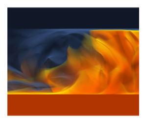
In figure 2 we compare a typical temperature field of the normal RB flow and that with homogeneous layers for  $Ra = 10^{6}$,
  $Pr = 1$ and
  $h = 0.2H$. We only show the fluid with temperature larger than
  $90\,\%\varDelta$ and smaller than
  $10\,\%\varDelta$. For normal RB flow at this relatively low
  $Ra$, the large thermal anomaly cannot be transported very far from the plates, which limits the global heat flux. On the contrary, with two homogeneous layers the plumes with large thermal anomaly are significantly stronger, and spread over the entire convection bulk. Accordingly, the heat flux is greatly enhanced in the flow with homogeneous layers. Although the strong thermal plumes shown in figure 2(b) are almost vertical, the large-scale circulations still exist between the two plates. In figure 3 we plot the time-averaged velocity field over a vertical slice. The streamlines clearly reveal a pair of large-scale convection rolls which extend from one plate to the other, including the homogeneous layers.

Figure 2. Volume rendering of the thermal field for  $Ra = 10^{6}$ and
  $Pr = 1$. Red and blue indicate the temperature larger than
  $90\,\%\varDelta$ and smaller than
  $10\,\%\varDelta$, respectively. Panel (a) shows the normal RB flow, and (b) shows the modified flow with two homogeneous layers of the height
  $h = 0.2H$.

Figure 3. The temporally averaged flow field on the  $y$–
$y$– $z$ plane at the middle location along the
  $x$ direction. Contours show the vertical velocity, and the streamlines are integrated with the in-plane velocity vector. The case is the same as the one shown in figure 2.
We then present the main results of the current study, i.e. the ultimate scalings (1.1a,b) for  $Nu$ and
  $Re$. To account for the homogeneous layers, the bulk Rayleigh number
  $Ra_b = Ra(1-2h/H)^{3}$ is used instead of
  $Ra$. The Nusselt and Reynolds numbers are calculated as
 \begin{equation} Nu = \frac{\left\langle w \theta \right\rangle_{bulk} - \kappa \partial_z \left\langle \theta \right\rangle_{bulk}}{\kappa \varDelta (H-2h)^{{-}1}},\quad Re = \frac{U_{rms}H}{\nu}, \end{equation}
where  $\langle \cdot \rangle _{bulk}$ stands for the average over the bulk region and time. We choose the root-mean-square value of the velocity magnitude as the characteristic velocity, which is calculated as
  $U_{rms}=\langle \boldsymbol {u}\boldsymbol {\cdot }\boldsymbol {u}\rangle ^{1/2}$. Here
  $\langle \boldsymbol {\cdot }\rangle$ is the average over the whole domain and time, since the flow motion is bounded by the two plates at
  $z=0$ and
  $H$. Note that when
  $h=0$ both
  $Ra_b$ and
  $Nu$ recover the original form for the RB flow.
We first look at the dependences of  $Nu$ and
  $Re$ on
  $Ra_b$ for fixed
  $Pr = 1$. Three decades of
  $Ra$ are covered from
  $10^{5}$ up to
  $10^{8}$. The height of the homogeneous layer is set at
  $h = 0.2 H$ so that for all simulations the momentum boundary layer is fully embedded inside the homogeneous layer. Figure 4 shows that both
  $Nu$ and
  $Re$ follow the ultimate scaling law (1.1a,b) perfectly, even though the Rayleigh number is not very large. Moreover, both the heat flux and flow velocity are greatly enhanced by introducing the homogeneous layers. For
  $Ra_b \geqslant 10^{6}$, the modified flow generates a heat flux more than one order of magnitude higher than that for the normal RB flow. For instance, the Nusselt number is comparable for the modified flow at
  $Ra \approx 10^{8}$ and the normal RB flow at
  $Ra \approx 10^{11}$.

Figure 4. The scaling of (a)  $Nu$ and (b)
  $Re$ vs
  $Ra_b$ for fixed
  $Pr = 1$ and increasing
  $Ra$. Solid symbols and lines depict the ultimate scaling of the modified flow with homogeneous layers. Open symbols and dashed lines show the normal RB flow and the classic scaling. The corresponding exponents are determined by linear fitting. The error bar is smaller than symbol size.
For the second group of simulations, we fix  $Ra = 3 \times 10^{6}$ and increase
  $Pr$ from
  $0.01$ to
  $10$, again covering three orders of magnitude. The height of the homogeneous layers is
  $h = 0.2H$. As shown in figure 5, the behaviours of
  $Nu$ and
  $Re$ are also very close to the ultimate scaling (1.1a,b). The scaling exponent for
  $Nu$ given by the linear fitting is indistinguishable from the theoretically predicted value
  $1/2$. The exponent for
  $Re$ obtained from the numerical data is slightly different from
  $-1/2$. For the moderate
  $Ra = 3\times 10^{6}$, the flow is not fully turbulent at the highest Prandtl numbers considered here. Therefore, Re decreases faster than that predicted by the ultimate scaling. Another interesting observation is that at low
  $Pr$ region, the difference between the modified flow and the normal RB flow is very small. This is expectable since for small
  $Pr$, the viscous boundary layer is thinner than the thermal one in the normal RB flow, and part of the thermal boundary layer is already in the turbulent bulk.

Figure 5. The scalings of (a)  $Nu$ and (b)
  $Re$ vs
  $Pr$ for fixed
  $Ra = 3\times 10^{6}$. The styles for symbols and lines are the same as figure 4. The error bar is smaller than symbol size.
To further demonstrate that the ultimate scaling is satisfied when the thermal and viscous boundary layers are decoupled from each other, we run simulations with increasing  $h$ for three different Rayleigh numbers
  $Ra = 10^{5}$,
  $10^{6}$ and
  $10^{7}$. The Prandtl number is fixed at
  $Pr = 1$. We focus on the behaviours of Nusselt number, which are shown in figure 6. As
  $h$ increases, i.e. the thermal boundary layers are gradually decoupled from the viscous ones, the heat flux is enhanced and the scaling exponent transits from the classic value of
  $1/3$ to the ultimate value
  $1/2$, see figure 6(a). It is interesting to notice that this transition is very similar to those reported for the radiative heating convection with increasing penetrating length (Bouillaut et al. Reference Bouillaut, Lepot, Aumaître and Gallet2019), and those for the oscillating convection with increasing frequency (Wang et al. Reference Wang, Zhou and Sun2020). In figure 6(b), we plot the scaling exponent
  $\gamma$ vs the height of the homogeneous layer
  $h$. For small
  $h$,
$h$,  $\gamma$ increases rapidly to a value larger than
  $1/2$. At this overshoot, the thermal boundary layer already enters the turbulent bulk for large
  $Ra$ but is still coupled with the viscous boundary layer for low
  $Ra$. Therefore, the heat flux is enhanced further for larger
  $Ra$ than the small ones, and the exponent is even bigger than
  $1/2$. When
  $h$ is large enough, for all three values of
  $Ra$, the thermal boundary layer is fully within the turbulent region, and the exponent
  $\gamma$ gradually approaches the value
  $1/2$.

Figure 6. (a)  $Nu$ vs
  $Ra_b$ for different
  $h$, which increases from
  $0$ to
  $0.2$ as colour changes from blue to red. (b) The scaling exponent
  $\gamma$ vs the height
  $h$. In both panels, the solid and dashed lines mark the ultimate scaling with the exponent
  $1/2$ and the classic scaling with the exponent
  $1/3$, respectively.
Figure 7 displays the profiles for four different  $Ra_b$ and fixed
  $Pr=1$. The profiles for mean temperature
  $\bar {\theta }(z)$, as shown in figure 7(a), demonstrate clearly the homogeneous layers at the top and bottom, the very thin thermal boundary layers adjacent to the homogeneous layers, and the bulk in the middle. Here the over line stands for averaging over the horizontal plane and time. For the two cases with smaller
  $Ra_b$, the gradient of the mean temperature is quite weak, similar to those of RB flows. However, for larger
  $Ra_b$, the mean temperature profiles have distinct gradient in the bulk, as observed in the vertical tube convection (Gibert et al. Reference Gibert, Pabiou, Chillà and Castaing2006, Reference Gibert, Culver, Dole-Olivier, Malard, Christman and Deharveng2009; Pawar & Arakeri Reference Pawar and Arakeri2016).

Figure 7. The profiles of (a) the mean temperature  $\bar {\theta }$ and (b–d) the standard deviation of temperature
  $\theta '$, one horizontal velocity component
  $u'$ and the vertical velocity
  $w'$, respectively. Different lines corresponds to different
  $Ra$, as indicated in panel (a). For all cases
  $Pr=1$ and
  $h=0.2H$.
The profiles of standard deviation are also shown for temperature, one horizontal velocity component and the vertical velocity in figure 7(b–d), respectively. The standard deviation for quantity  $\zeta$ is calculated as
  $\zeta '=(\overline {\zeta -\bar {\zeta }})^{1/2}$, which measures the level of fluctuation around the mean value. In the convection region between the two homogeneous layers,
  $\theta '$ is nearly constant. The value in the thermal boundary layer is only slightly larger than that in the bulk. The viscous boundary layer, which is defined as the region between the peak location of the
  $u'$ profile and the corresponding plate, locates entirely inside the homogeneous layer. Therefore, the thermal boundary layers are shifted into the turbulent bulk. The profiles of
  $u'$ and
  $w'$ have similar magnitude in the bulk, indicating a nearly isotropic turbulent state.
The boundary-layer thickness  $\delta$ is extracted by the peak location in the standard deviation profiles of temperature and the horizontal velocity component. Figure 8 displays the dependence of
  $\delta _u$ and
  $\delta _\theta$ on
  $Ra_b$ and
  $Pr$. For fixed
  $Pr=1$ and
  $h=0.2H$, as shown in figure 8(a), the viscous boundary-layer thickness
  $\delta _u$ does not have a clear scaling law over
  $Ra_b$. The three cases with smaller
  $Ra_b$ and the four cases with larger
  $Ra_b$ form two groups and a sudden change appears between
  $Ra_b=2.16\times 10^{5}$ and
  $6.48\times 10^{5}$. The exact reason for this is not clear yet. Two competing effects are introduced into the momentum field by the homogeneous layers. On one hand, the homogeneous layers greatly enhance the velocity of convection motions which should reduce
  $\delta _u$. On the other hand, fluid has to penetrate the homogeneous layer and reach the plate purely by inertia since buoyancy force is turned off in this layer, which weakens the velocity near the plate and increases
  $\delta _u$. Then a certain transition may appear when the dominant effect changes from one to the other. For fixed
  $Ra_b=6.48\times 10^{5}$ and increasing
  $Pr$, as shown in figure 8(b),
  $\delta _u$ increases due to the reduction of
  $Re$.
$Re$.

Figure 8. The thickness of the thermal boundary layer  $\delta _\theta$ (red solid symbols) and the viscous one
  $\delta _u$ (blue open symbols) vs (a)
  $Ra_b$ and (b)
  $Pr$. In (a),
  $Pr=1$ and in (b),
  $Ra_b=6.48\times 10^{5}$. Scaling laws are shown by the dashed lines with derived exponents.
The behaviours of  $\delta _\theta$ depicted in figure 8 can be described by the scaling analysis developed in Grossmann & Lohse (Reference Grossmann and Lohse2004) for RB flows, where the thermal boundary-layer thickness obeys
 \begin{equation} \delta_\theta / H \sim F(Pr) Re^{{-}1/2} Pr^{{-}1/3}. \end{equation}
The function  $F(Pr)$ has different asymptotic behaviours for
  $Pr\ll 1$ and
  $Pr\gg 1$. For fixed
  $Pr$, one always has
  $\delta _\theta /H \sim Re^{-1/2} \sim Ra_b^{-0.250}$, in which we have used the scaling law
  $Re \sim Ra_b^{0.5}$. For fixed
  $Ra_b$ and
  $Pr\gg 1$,
  $F(Pr)=1$ and one obtains
  $\delta _\theta /H\sim Re^{-1/2}Pr^{-1/3}=Pr^{-0.083}$, in which we have used the scaling law
  $Re \sim Pr^{-0.5}$. While for
  $Pr\ll 1$, one has
  $\delta _\theta /H\sim Re^{-1/2}Pr^{-1/2}=Pr^{-0.250}$. The three scaling laws are plotted in figure 8 and compared with the numerical results. The agreement between the numerical data and the three scaling laws is good. In our simulations, although the thermal boundary layer locates within the turbulent bulk, the viscous boundary layer itself is still laminar. The above scaling laws were originally developed for laminar boundary layer, which may be the reason why these scaling laws still hold in the current configuration.
As a final demonstration of the turbulent state of the flow, we calculate the energy spectra for temperature and velocity components over the horizontal plane at the mid height, see figure 9. The energy spectrum for quantity  $\zeta$ is calculated as
  $E_{\zeta} (k) = \sum_{|\boldsymbol{k}|=k} (\tilde{\zeta}(\boldsymbol{k})\tilde{\zeta}^*(\boldsymbol{k})/2)$. Here,
  $\boldsymbol{k}$ is the wavenumber vector. The tilde stands for the complex coefficients after the discrete Fourier transform, and
  $^*$ for the complex conjugate, respectively. Here,
  $\zeta$ can be
  $\theta,\ u$ or
  $w$. The energy spectra are averaged over time and normalized by the respective total fluctuation energy. As
  $Ra_b$ increases, more and more small scale modes are excited. A short inertial range with a slope close to
  $-5/3$ can be observed, especially for large
  $Ra_b$.

Figure 9. (a) The energy spectra of  $\theta$. (b) The energy spectra for
  $u$ (dashed lines) and
  $w$ (solid lines). Blue lines are for
  $Ra_b = 2.16\times 10^{5}$, red lines for
  $Ra_b=2.16\times 10^{6}$ and black lines for
  $Ra_b = 2.16\times 10^{7}$, respectively. For all cases
  $Pr=1$.
4. Conclusions and discussions
In summary, we demonstrate that once the thermal boundary layers decouple with the viscous ones and locate within the turbulent convection bulk, the scaling laws of the heat flux and flow velocity are very close to those predicted for the ultimate regime even at relatively low Rayleigh numbers. Our results are consistent with the physical picture about the ultimate state of convection turbulence, namely when the momentum boundary layers become fully turbulent, the heat flux is independent of the fluid viscosity. The current flow can be regarded as a realization of the IV $_l$ regime within the unifying model for RB convection (Grossmann & Lohse Reference Grossmann and Lohse2000, Reference Grossmann and Lohse2001, Reference Grossmann and Lohse2002, Reference Grossmann and Lohse2004), saying the viscous and thermal dissipations are both dominated by the bulk region. Compared with the homogeneous convection (Lohse & Toschi Reference Lohse and Toschi2003; Calzavarini et al. Reference Calzavarini, Lohse, Toschi and Tripiccione2005, Reference Calzavarini, Doering, Gibbon, Lohse, Tanabe and Toschi2006), the current flow configuration achieves the ultimate scaling with the thermal boundary layers still evolved, and avoids the exponentially growing modes in the fully periodic simulations. The current study provides a new type of model system for the investigation of the convection turbulence with very strong thermal driving.
Of course, a definitive proof for the existence of the ultimate regime relies on the direct observation of the ultimate scaling in the experiments and simulations of the normal RB convection. We also admit that the flow configuration proposed here may be difficult to be realized by experimental study. Nevertheless, one can anticipate that, based on the present study, convection flows will probably enter the ultimate state when the boundary-layer region becomes fully turbulent at extremely high thermal driving. Such conditions are very likely satisfied in natural systems such as the Earth outer core and stars. Transition towards the ultimate regime has been reported in recent studies (He et al. Reference He, Funfschilling, Nobach, Bodenschatz and Ahlers2012; Zhu et al. Reference Zhu, Stevens, Verzicco and Lohse2017, Reference Zhu, Mathai, Stevens, Verzicco and Lohse2018, Reference Zhu, Stevens, Shishkina, Verzicco and Lohse2019), and we may expect that a fully developed ultimate state will be observed in experiments in the near future.
Acknowledgements
The authors appreciate the helpful discussions with D. Lohse, R. Verzicco and K.-Q. Xia, and the valuable comments from the anonymous referees. The volume rendering is generated by the open source software VisIt (Childs et al. Reference Childs2012).
Funding
This work is supported by the Major Research Plan of National Natural Science Foundation of China for Turbulent Structures under the grants 91852107 and 91752202. Y.Y. also acknowledges the partial support from the Strategic Priority Research Program of Chinese Academy of Sciences under the grant no. XDB42000000.
Declaration of interests
The authors report no conflict of interest.
Appendix. Details of simulations performed in the horizontally periodic domain
In this Appendix we summarize the numerical details. Here,  $\varGamma$ is the aspect ratio, and
  $N_x(m_x)$ and
  $N_z(m_z)$ are the resolutions of base mesh (and the refinement factor) in the horizontal and vertical directions, respectively. The Nusselt number, Reynolds number and thicknesses of boundary layers are also listed in tables 1–3. The domain width and the meshes are the same in the two horizontal directions.
Table 1. Cases with different  $Ra_b$ and fixed
  $Pr = 1$.

Table 2. Cases with different  $Pr$ and fixed
  $Ra = 3\times 10^{6}$.

Table 3. Cased with different  $h$,
$h$,  $Ra_b$ and fixed
  $Pr = 1$.


