


1. Introduction
Gas flow in microchannels linking large reservoirs is a fundamental problem of rarefied gas dynamics underpinning the development of microsystems. Although the rarefied gas flow in a straight microchannel has been extensively investigated (Sharipov & Seleznev Reference Sharipov and Seleznev1998; Sazhin Reference Sazhin2009; Titarev Reference Titarev2012a,Reference Titarevb; Varoutis, Day & Sharipov Reference Varoutis, Day and Sharipov2012), only a few experimental (Lee, Wong & Zohar Reference Lee, Wong and Zohar2001; Varade et al. Reference Varade, Agrawal, Prabhu and Pradeep2015) and numerical (Raju & Roy Reference Raju and Roy2004; Wang & Li Reference Wang and Li2004; Agrawal, Djenidi & Agrawal Reference Agrawal, Djenidi and Agrawal2009; Sharipov & Graur Reference Sharipov and Graur2012; White et al. Reference White, Borg, Scanlon and Reese2013; Kulakarni, Shterev & Stefanov Reference Kulakarni, Shterev and Stefanov2015; Rovenskaya Reference Rovenskaya2016; Liu et al. Reference Liu, Tang, Su, Wu and Zhang2018) studies have been carried out for rarefied gas flows through a microchannel with bends, which are often encountered in miniaturised devices. One of the typical phenomena in bent channels is flow separation, which is important for many engineering applications and has been studied extensively in the continuum limit (Bradshaw & Wong Reference Bradshaw and Wong1972). In the literature, flow recirculation, vortex formation or secondary flow is also often used to describe flow separation phenomena. However, much less attention has been paid to flow separation in microsystems, as the Reynolds number  $Re$ is often small. Moreover, the Knudsen number
  $\textit{Kn}$, which is defined as the ratio between the mean free path of gas molecules and the characteristic flow length, is not always small, resulting in a new mechanism for flow separation which does not appear in macrosystems. For example, in an early work on gas flow separation in a bent microchannel (Lee et al. Reference Lee, Wong and Zohar2001), the experimentally measured data at a fixed Knudsen number at the channel exit
  $(\textit{Kn}_e=0.06)$ showed that the mass flow rate ratio between the bent and straight channels of the same length, i.e.
 \begin{equation} \alpha=\frac{G_{bent}}{G_{straight}} \end{equation}
is close to  $0.8$, when the pressure ratio
 \begin{equation} \beta=\frac{p_{e}}{p_{i}}, \end{equation}
between the exit and the inlet varies from  $0.25$ to
  $0.33$. Moreover, the pressure gradients around the concave and convex corners are nearly zero and positive, respectively, indicating that the flow separation or vortex generation at both corners, as illustrated in figure 1, may exist even at very low Reynolds numbers, i.e.
  $Re \le 0.06$. This critical value of Reynolds number is three orders of magnitude smaller than the lowest Reynolds number (approximately
  $100$ to
  $300$) in the continuum flow for the emergence of flow separation (Maharudrayya, Jayanti & Deshpande Reference Maharudrayya, Jayanti and Deshpande2004; Xiong & Chung Reference Xiong and Chung2008).

Figure 1. Schematic of laminar flow separation (vortex formation) in a microchannel with a rectangular bend.
The pioneering experimental work of Lee et al. (Reference Lee, Wong and Zohar2001) inspired the numerical investigations to understand rarefied gas flow in bent microchannels, but many contradictory results are reported, which are summarised in table 1. Flow separation at the concave corner is, surprisingly, captured by Agrawal et al. (Reference Agrawal, Djenidi and Agrawal2009), White et al. (Reference White, Borg, Scanlon and Reese2013) and Varade et al. (Reference Varade, Agrawal, Prabhu and Pradeep2015) at low Reynolds numbers using the lattice Boltzmann method, the direct simulation Monte Carlo (DSMC) method (Bird Reference Bird1994) and the Navier–Stokes solver, respectively. Small recirculation at the bends can be deduced from the velocity profiles obtained in the numerical simulation of the Navier–Stokes equations with the first-order slip velocity boundary condition (Raju & Roy Reference Raju and Roy2004). However, the others explicitly confirmed that no trace of flow separation was found using the DSMC method (Wang & Li Reference Wang and Li2004) and the discrete velocity method (DVM) of solving the linearised kinetic equations (Sharipov & Graur Reference Sharipov and Graur2012; Liu et al. Reference Liu, Tang, Su, Wu and Zhang2018).
Table 1. Contradictory reports in the literature about existence of vortex in microchannels and mass flow rate ratio  $\alpha$. Here, *:
  $\alpha$ is almost constant with increasing pressure ratio
  $\beta$; **:
  $\alpha$ increases monotonically with pressure ratio
  $\beta$; ***:
  $\alpha$ decreases monotonically with increasing mean Knudsen number
  $\textit{Kn}_{m}$. Subscripts ‘
 $i$’, ‘
 $e$’ and ‘
 $m$’ in the
  $\textit{Kn}$ range indicate the inlet, exit and mean Knudsen number, respectively. Abbreviations ‘E’, ‘N.M.’ and ‘N.A.’ mean ‘expected’, ‘not mentioned’ and ‘not available’, respectively.

Table 1 further shows that the mass flow rate ratio  $\alpha$ is reported in the literature in a rather scattered fashion. Raju & Roy (Reference Raju and Roy2004) showed that
  $\alpha$ varies from
  $0.38$ to
  $0.52$ when the pressure ratio
  $\beta$ is increased and
  $\textit{Kn}_{e}$ is fixed around 0.06. The others reported that
  $\alpha$ is very close to unity or slightly higher than unity in the slip flow regime. Also, it varies differently with respect to the Knudsen number: Liu et al. (Reference Liu, Tang, Su, Wu and Zhang2018) reported that
  $\alpha$ decreases monotonically when
  $\textit{Kn}$ increases; White et al. (Reference White, Borg, Scanlon and Reese2013) found the steep increase of
  $\alpha$ to its maximum value at the inlet Knudsen number of
  $\textit{Kn}_{i}=0.027$, followed by a gradual decrease; Agrawal et al. (Reference Agrawal, Djenidi and Agrawal2009) and Rovenskaya (Reference Rovenskaya2016) observed a steep increase of
  $\alpha$ to its maximum value at
  $\textit{Kn}_{e}=0.2$ and
  $0.05$, then remaining plateaued up to
  $\textit{Kn}_{e}=0.5$ and 0.1, respectively. This small flow rate enhancement in the bent channel compared with the straight channel has been attributed to numerical uncertainty (Agrawal et al. Reference Agrawal, Djenidi and Agrawal2009), reduction of average shear stress (White et al. Reference White, Borg, Scanlon and Reese2013; Rovenskaya Reference Rovenskaya2016) or cross-section expansion at the bends (Liu et al. Reference Liu, Tang, Su, Wu and Zhang2018). As no vortex is found in the detailed flow structure analysis, the case of flow rate ratio
  $\alpha$ less than unity is attributed to rarefaction effect rather than flow separation (Wang & Li Reference Wang and Li2004). On the other hand, when the exit Knudsen number is fixed at
  $\textit{Kn}_e\approx 0.06$, the mass flow rate ratio
  $\alpha$ increases considerably with the pressure ratio
  $\beta$ (Raju & Roy Reference Raju and Roy2004), which contradicts the experimental observation of the constant ratio (Lee et al. Reference Lee, Wong and Zohar2001).
It is the aim of the present work to elucidate the contradictory findings on flow separation and flow rate enhancement due to bent channels through a thorough numerical study covering a wide range of Knudsen numbers and Reynolds numbers. To ensure computational accuracy, the kinetic equation is solved by the deterministic DVM with very refined spatial resolution.
2. Problem statement and gas kinetic simulation
2.1. Statement of the problem
Consider the rarefied flow of argon gas through the straight and bent channels of the same height  $h$ and axis length
  $L_{ch}=5h$ connecting the two reservoirs of equal size, see figure 2. The gas pressures in the upstream and downstream reservoirs are
  $p_{i}$ and
  $p_{e}$, respectively. The reservoir gas and wall temperatures are kept at
  $T_0=273\ \text {K}$. The resulting rarefied gas flow is characterised by the pressure ratio
  $\beta$ and the reference Knudsen number
 \begin{equation} \textit{Kn}=\frac{\lambda}{L_{0}},\quad\lambda=\frac{\mu_{0}}{p_{0}}\sqrt{\frac{{\rm \pi} k_{B}T_{0}}{2m}}, \end{equation}
where  $\mu _0$,
  $\lambda$,
  $m$ and
  $k_{B}$ are the gas viscosity at temperature
  $T_0$, the molecular mean free path, the molecular mass and the Boltzmann constant, respectively. The channel height and the inlet pressure are taken as the reference length
  $L_0=h$ and the reference pressure
  $p_0=p_i$, respectively. As a result, our reference Knudsen number is the inlet Knudsen number
  $\textit{Kn} = \textit{Kn}_i$. When the exit or mean Knudsen number (
 $\textit{Kn}_e$ or
  $\textit{Kn}_m$) is of interest, it can be calculated from the reference Knudsen number and pressure ratio
  $\beta$, i.e.
  $\textit{Kn}_e=\textit{Kn} / \beta$ or
  $\textit{Kn}_m = \textit{Kn}(1+\beta )/(2\beta )$, respectively. Alternatively, the gas rarefaction can be characterised by the rarefaction parameter
  $\delta$, which relates to
  $\textit{Kn}$ as
  $\delta ={\sqrt {{\rm \pi} }L_{0}}/{2\lambda }={\sqrt {{\rm \pi} }}/{2\textit{Kn}}$.

Figure 2. Pressure-driven gas flow from the left-hand reservoir to the right-hand reservoir through (a) the straight channel and (b) the bent channel of the same height  $h$ and axis length
  $L_{ch}=5h$. Note that only part of the reservoirs are illustrated here.
The effect of pressure ratio can be reflected by the Reynolds number  $Re$ that is defined as
 \begin{equation} Re=\frac{\rho_0U_0L_0}{\mu_0}, \end{equation}
where  $U_0$ is the characteristic flow speed, e.g. the average speed in the channel and
  $\rho _0=mp_0/(k_{B}T_0)$ is the reference density. The Mach number
  $Ma$ relates to the Knudsen number
  $\textit{Kn}$ and the Reynolds number
  $Re$ through the von Kármán relation
 \begin{equation} Ma=\sqrt{\frac{2}{{\rm \pi}\gamma}}\textit{Kn}Re, \end{equation}
where the specific heat ratio  $\gamma$ is taken to be
  $5/3$ for monatomic gas.
2.2. The governing equation and boundary condition
The Boltzmann equation is the fundamental equation to describe the rarefied dynamics of monatomic gas. However, due to the complexity of its collision operator, the kinetic model (Shakhov Reference Shakhov1968) is often used to simulate rarefied gas flows. Without an external body force, the Shakhov model equation takes the following form:
 \begin{equation} \frac{\partial f}{\partial t} + \boldsymbol c \boldsymbol{\cdot} \boldsymbol{\nabla} f = \frac{ f^S-f}{\tau}. \end{equation}
Here  $f = f(\boldsymbol x,\boldsymbol c, t)$ is the velocity distribution function of gas molecules with molecular velocity
  $\boldsymbol c = (c_x, c_y, c_z)$ at position
  $\boldsymbol x = (x, y, z)$ and time
  $t$, and the reference distribution function
  $f^S$ reads
 \begin{equation} f^{S}= \frac{n}{(2{\rm \pi} k_{B}T/m)^{3/2}}\exp\left( - \frac{m\xi^2}{2k_{B}T} \right) \left[1+\left(1-Pr\right)\frac{m\boldsymbol{\xi}\boldsymbol{\cdot}\boldsymbol q}{5n\left(k_{B}T\right)^{2}} \left(\frac{m\xi^{2}}{k_{B}T}-5\right)\right],\end{equation}
where  $n$ and
  $T$ are the gas number density and temperature, respectively,
  $\boldsymbol \xi = \boldsymbol c - \boldsymbol u$ is the peculiar velocity, with
  $\boldsymbol u$ the macroscopic flow velocity and
  $\boldsymbol q=({m}/{2})\int \boldsymbol {\xi }\xi ^{2}f\,\text {d}\boldsymbol c$ is the heat flux. The Prandtl number
  $Pr$ is set to be
  $2/3$ for monatomic gas. Conservative flow variables are calculated as
  $\boldsymbol W \equiv (n, n\boldsymbol u, ne)^{\textrm {T}}=\int \boldsymbol ( 1, \boldsymbol c, c^2/2 )^{\textrm {T}} f \,\text {d}\boldsymbol c$ and the temperature is determined from the specific total energy
  $e = (u^2 + 3k_{B}T/m)/2$.
The relaxation time  $\tau$ in the Shakhov model (2.4) is related to the dynamic viscosity
  $\mu$ and the local pressure
  $p$ as
  $\tau = \mu /p=\mu /(nk_{B}T)$. For gas molecules interacting through the inverse power law potential, the dynamic viscosity
  $\mu$ depends on the temperature
  $T$ as
 \begin{equation} \mu=\mu_{0}\left(\frac{T}{T_{0}}\right)^{\omega}, \end{equation}
where  $\omega$ is the viscosity index. Argon gas with
  $m=6.63 \times 10^{-26}$ kg,
  $\mu _0=2.117 \times 10^{-5}$ Ns m
 $^{-2}$ and
  $\omega =0.81$ is considered in this paper.
To simulate the rarefied gas flow, the gas–surface interaction should be specified, which is modelled by the Maxwell diffuse–specular reflection, i.e.
 \begin{align} f\left(\boldsymbol{c} \mid \boldsymbol{c} \boldsymbol{\cdot} \boldsymbol{N} > 0 \right)&=\alpha_d n_s \left(\frac{m}{2{\rm \pi} k_{B}T_0}\right)^{3/2}\exp\left(-\frac{mc^2}{2k_{B}T_0}\right) \nonumber\\ &\quad + \left(1-\alpha_d\right)f\left[ \boldsymbol{c}-2\boldsymbol{N} (\boldsymbol{c} \boldsymbol{\cdot} \boldsymbol{N})\right],\quad (0\le\alpha_d\le 1), \end{align}
where  $\boldsymbol {N},n_s,\alpha _d$ are the normal unit vector of the solid surface, the gas number density on the solid surface and the accommodation coefficient, respectively. In the diffuse–specular model,
  $\alpha _d$ portion of incident particles are reflected diffusively, whereas the remaining
  $(1-\alpha _d)$ portion of incident particles have a specular reflection. The diffuse boundary condition
  $\alpha _d=1$ at the solid surfaces is used in this study, except for the simulations in § 3.2 where diffuse–specular reflection is used. The gas number density on the solid surface is computed from the non-penetration condition, i.e. the number of gas molecules reflected from the wall is equal to those molecules approaching the same wall
 \begin{equation} n_s=-2\sqrt{\frac{\rm \pi}{2k_BT_0/m}}\int_{\boldsymbol{c} \boldsymbol{\cdot} \boldsymbol{N} < 0}\boldsymbol{c}\boldsymbol{\cdot} \boldsymbol{N} f \,{\mathrm{d}\boldsymbol{c}}. \end{equation}
 At the free surfaces of reservoirs, molecules entering the computational domain follow the Maxwellian distribution with the local bulk velocity  $\boldsymbol {u}$, pressure and temperature corresponding to each reservoir. The local velocity
  $\boldsymbol {u}$ at the free surfaces is extrapolated from that of the interior neighbour grid points.
2.3. The numerical methods
We employ the reference length  $L_0$, temperature
  $T_0$, pressure
  $p_0$ and the most probable molecular speed
  $v_m=\sqrt {2k_{B}T_0/m}$ to normalise the following variables:
 \begin{equation} \left(\tilde{X},\tilde{Y}\right)=\frac{\left(X,Y\right)}{L_0},\quad \left(\tilde{u},\tilde{v}\right)=\frac{\left(u,v\right)}{v_m},\quad \tilde{T}=\frac{T}{T_0},\quad \tilde{p}=\frac{p}{p_0},\quad \tilde{n}=\frac{n}{p_0/k_BT_0}, \end{equation}
where  $u$ and
  $v$ are the velocity components of macroscopic velocity
  $\boldsymbol u$ along the coordinate axes
  $X$ and
  $Y$, respectively. Hereafter, the tildes on these dimensionless quantities are omitted for simplicity.
The DVM is one of the most commonly used deterministic approaches to solving the Boltzmann equation and its simplified models (Broadwell Reference Broadwell1964; Yang & Huang Reference Yang and Huang1995). It projects the continuous molecular velocity space  $\boldsymbol c$ into a set of discrete velocities
  $\boldsymbol c^{(i)}$
 $(i=1,2,\ldots ,N_{c})$. As a result, the governing equation (2.4) is replaced by a system of
  $N_{c}$ independent equations. Here, we discretise this system in time by a time-implicit Godunov-type scheme (Yang & Huang Reference Yang and Huang1995; Titarev Reference Titarev2007)
 \begin{equation} \left.\begin{gathered} \left[\frac{1}{{\rm \Delta}{t^{(j)}}}+{\boldsymbol c^{(i)}}\boldsymbol{\cdot} \boldsymbol{\nabla}+\frac{1}{\tau^{(j)}}\right]{\rm \Delta} f^{(j)}=\text{RHS}^{(j)}, \\ \text{RHS}^{(j)}=\frac{1}{\tau^{(j)}}\left[f_{eq}^{(j)}-f^{(j)}\right]-{\boldsymbol c^{(i)}}\boldsymbol{\cdot} \boldsymbol{\nabla} f^{(j)}, \end{gathered}\right\} \end{equation}
where  ${\rm \Delta} f^{(j)}=f^{(j+1)}-f^{(j)}$ needs to be determined at the time step
  ${\rm \Delta} {t^{(j)}}$ and
  $j$ is the time step index. Here,
  $\text {RHS}^{(j)}$ is the explicit part, and the spatial derivative is approximated by a third-order upwind scheme. This time-implicit scheme allows us to use a large time step to accelerate steady-state solution. Specifically, the classical Courant–Friedrichs–Lewy number of
  $10^6$ is chosen in this study. A few efficient implicit methods for solving the linearised Shakhov model have been developed by Titarev (Reference Titarev2012a,Reference Titarevb, Reference Titarev2013). The details of the DVM algorithm used in this work can be found in Ho et al. (Reference Ho, Li, Wu, Reese and Zhang2019). In the following simulations, the polar velocity grids of
  $N_c = N_{c_p} \times N_{\varphi }= 4\times 120$ and
  $4\times 40$ are chosen for
  $\textit{Kn}>0.1$ and
  $\textit{Kn} \le 0.1$, respectively. The number of discretised velocities in the angular coordinate
  $N_{\varphi }$ is uniformly spaced on
  $[0,2{\rm \pi} ]$, whereas the number of discretised velocities in the radial coordinate
  $N_{c_p}$ follows the half-range Gauss–Hermite abscissae. The molecular velocity is cut off at
  $2.3$ times the most probable molecular speed
  $v_m$ with
  $N_{c_p}=4$. In the cases of small pressure ratio, i.e.
  $\beta =0.75, 0.5$ and low Knudsen number
  $\textit{Kn} \le 0.03$,
  $N_{c_p}=8$ and the truncated molecular velocity of
  $3.7v_m$ are used due to relatively high Mach number. With these sets of the velocity grids, the numerical uncertainty is of the order of
  $0.1\,\%$ when
  $N_{c_p}$ is doubled (note: the truncated molecular velocity is also enlarged accordingly).
Different uniform spatial grids are used in DVM simulations based on the value of Knudsen number, i.e.  $L10W4h160$,
  $L20W8h80$ and
  $L40W16h40$ are used for
  $\textit{Kn} \le 0.1$,
  $0.1 < \textit{Kn} \le 1$ and
  $1 < \textit{Kn}$, respectively. Here, for example, the spatial grid
  $L10W4h160$ denotes the reservoirs are of size of
  $L=10h$,
  $W=4h$ and the reference length (i.e. the channel height
  $h$) is resolved by
  $160$ uniform-cells, see figure 2.
Our simulations start from the global equilibrium state. The convergence criterion for the steady-state is checked every time step as follows:
 \begin{equation} E(t)=\frac{\sum \left|\boldsymbol{u}(t)-\boldsymbol{u}(t-{\rm \Delta} t)\right|}{\sum |\boldsymbol{u}(t)|}<10^{-6}. \end{equation}
 The reduced mass flow rate  $G$, normalised by
  $h^2(p_{i}-p_{e})/v_{m}L_{ch}$, reads
 \begin{equation} G=\frac{L_{ch}}{h}\frac{2p_0}{\left(p_{i}-p_{e}\right)} \int nu\,\text{d}Y=\frac{L_{ch}}{h}\frac{2p_0}{\left(p_{i}-p_{e}\right)}u_{avg}.\end{equation}
The average speed  $u_{avg}=\int nu\,\text {d}Y$ is calculated at two vertical cross-sections inside the channel near the inlet and the exit to guarantee the mass conservation. The discrepancy of
  $u_{avg}$ near the inlet and the exit is less than
  $0.01\,\%$. To calculate the Reynolds number, the characteristic flow speed
  $U_0$ in (2.2) is determined by
  $U_0=u_{avg}v_m$.
In this study, DVM is used for solving the nonlinear Shakhov model, see (2.4) and (2.5) for all the values of pressure ratio  $\beta$, except for
  $\beta =0.99999$. For
  $\beta =0.99999$, the DVM simulation converges very slowly and requires a very fine spatial grid at such low
  $\textit{Kn}$ (Valougeorgis & Naris Reference Valougeorgis and Naris2003; Wang et al. Reference Wang, Ho, Wu, Guo and Zhang2018). Therefore, the discontinuous Galerkin method (DGM) and general synthetic iterative scheme, which enables the fast convergence to the steady-state solution and retains asymptotic preserving natures of the Navier–Stokes equations, is employed to solve the linearised Shakhov equation for the case of pressure ratio
  $\beta =0.99999$ (Su et al. Reference Su, Wang, Zhang and Wu2019b, Reference Su, Zhu, Wang, Zhang and Wu2020b). The DVM and DGM solutions are compared with each other and with the other available data, see appendix A.
3. Flow separation at bends
In this section, we numerically investigate the gas flow through the bent channel over a wide range of Knudsen and Reynolds numbers. In particular, the role of velocity slip on the flow separation (vortex formation) is evaluated.
3.1. Influence of Reynolds number and Knudsen number
In our simulations, the Knudsen number  $\textit{Kn}$ and the pressure ratio
  $\beta$ are chosen first, and the Reynolds number
  $Re$ is then obtained from the simulation results. The compressibility of the gas tends to suppress vortices generation which has been observed in supersonic flows, e.g. see Burggraf (Reference Burggraf1966). The compressibility effects may be insignificant as the Mach number
  $Ma$ calculated from the von Kármán relation (2.3) is up to
  $1.5\times 10^{-3}$,
  $1.5\times 10^{-2}$,
  $0.19$ and
  $0.25$ for all the considered cases of the pressure ratio
  $\beta =0.99999$,
  $0.99$,
  $0.75$ and
  $0.5$, respectively.
Figure 3 shows the streamlines and the pressure distribution inside the bent channel for  $\textit{Kn}=0.01$,
  $0.02$ and
  $0.05$ with the pressure ratio
  $\beta =0.99$ and
  $0.5$. With the fixed pressure ratio
  $\beta$ and increasing
  $\textit{Kn}$,
  $Re$ becomes smaller so that the vortices at the bends shrink or even disappear. The strong influence of
  $Re$, i.e. the inertial effect from the mainstream, on the vortex formation is well known for continuum flows; however, with the presence of gas rarefaction effect in microflow, two unusual phenomena are observed in figure 3. First, the Reynolds number alone cannot characterise the flow separation in a microchannel. For example, from figures 3(c) and 3(f) we see that in the slip flow regime the vortices exist at
  $Re=0.68$ but not at a larger
  $Re$ of
  $4.72$. Second, as shown in figures 3(c) and 3(b), the vortices near the concave and convex corners occur at
  $Re$ as small as
  $0.68$ and
  $40.65$, respectively, while the corresponding critical Reynolds numbers (i.e. the smallest
  $Re$ where the vortex emerges) for air in the continuum flow regime, obtained from the Navier–Stokes equations with a no-slip boundary condition (Maharudrayya et al. Reference Maharudrayya, Jayanti and Deshpande2004), are
  $200$ and
  $100$; on the other hand, for water flow in a microchannel no vortex is observed experimentally when
  $Re<100$ (Xiong & Chung Reference Xiong and Chung2008). To analyse these contradictory observations, we need to look into the secondary flows at the bends.

Figure 3. The pressure field and streamlines of rarefied argon gas flow inside the bent channel at different values of  $\textit{Kn}$ and
  $Re$. Note: the rarefaction
  $\delta$ of
  $88.6, 44.3, 17.7$ corresponds to
  $\textit{Kn}=0.01, 0.02, 0.05$, respectively. (a)
  $\beta = 0.99, \textit{Kn}= 0.01, Re= 2.48$; (b)
  $\beta = 0.5, \textit{Kn}= 0.01, Re= 40.65$; (c)
  $\beta = 0.99, \textit{Kn}= 0.02, Re= 0.68$; (d)
  $\beta = 0.5, \textit{Kn}= 0.02, Re= 17.80$; (e)
  $\beta = 0.99, \textit{Kn}= 0.05, Re= 0.13$ and (f)
  $\beta = 0.50, \textit{Kn} = 0.05, Re= 4.72$.
To the best of authors’ knowledge, the concave vortex, which exists near the concave corners, is closely related to the Moffatt eddies originally found by the Stokes stream function for viscous fluid near deep sharp corners in Stokes flow (Moffatt Reference Moffatt1964). Contrary to the conventional vortex occurring at high  $Re$, where the centrifugal force is balanced by the pressure force, the Moffatt viscous vortex is both driven and damped by the viscous force. By solving the stream function in the Stokes limit at the vicinity of a sharp corner, Moffatt found that a sequence of vortices generally appears if the angle of the sharp corner is smaller than the critical angle
  $146^\circ$. In the hydrodynamic regime, Moffatt eddies have been confirmed numerically by Biswas, Breuer & Durst (Reference Biswas, Breuer and Durst2004) in backward-facing step flows, where the primary vortex has been observed in a wide range of
  $Re$ from
  $10^{-4}$ to
  $10^2$. Interestingly, the vortex size is nearly constant when the Reynolds number increases up to unity, then becomes larger with a further increase of
  $Re$ (up to
  $100$). Also, the size ratio of the primary vortex to the secondary vortex obtained by their Navier–Stokes simulations for
  $Re=1$ is in good agreement with the Stokes approximation in the Moffatt analysis (
 $16.28$ for the right angle corner). This rapid reduction of the size of successive vortices leads to enormous difficulty in capturing a sequence of vortices experimentally. In gas microflow, the concave vortex was, surprisingly, observed in the numerical simulations with
  $Re$ of the order of unity (Agrawal et al. Reference Agrawal, Djenidi and Agrawal2009; White et al. Reference White, Borg, Scanlon and Reese2013). Without awareness of Moffatt's theory, the existence of a concave vortex at such low
  $Re$ is either attributed to gas rarefaction (Agrawal et al. Reference Agrawal, Djenidi and Agrawal2009) or not acknowledged (Wang & Li Reference Wang and Li2004; Sharipov & Graur Reference Sharipov and Graur2012; Liu et al. Reference Liu, Tang, Su, Wu and Zhang2018). We observe, for the first time, that the concave vortex in gas microflows does exist in the limit as the Reynolds number approaches zero, which agrees with Moffatt's theory. From our simulations, the smallest Reynolds number for a vortex to appear is found to be
  $0.32\times 10^{-3}$ for the case of pressure ratio
  $\beta =0.99999$ and
  $\textit{Kn}=0.03$, as shown in figure 4(a).

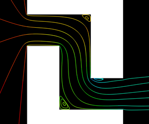
Figure 4. Critical values of the Reynolds number for the emergence of (a) concave vortex (enlarged view of the pressure field and streamlines near the first concave corner of the upper wall) and (b) convex vortex. Note: the rarefaction  $\delta$ of
  $88.6,29.5$ corresponds to
  $\textit{Kn}=0.01, 0.03$, respectively. (a)
  $Re= 0.32\times 10^{-3}, \textit{Kn}= 0.03, \beta = 0.99999$ and (b)
  $Re= 30.8, \textit{Kn}= 0.01, \beta = 0.75$.
The convex vortex, which appears in the downstream side of convex bent corners, is formed when the fluid streams cannot move closely along the sharp angle of the wall after the convex corner due to their relatively high momentum. The flow separation emerges from the convex corner point and extends beyond the vena contracta, i.e. the narrowest region of the stream after a sudden contraction of the duct (see the schematic diagram in figure 1). A similar effect is also observed in the slip flow through an orifice (Sharipov Reference Sharipov2004; Ho & Graur Reference Ho and Graur2014). This type of vortex was observed clearly from the experiments of water flow through a microchannel with bends at  $Re \ge 300$ (Xiong & Chung Reference Xiong and Chung2008). To the best of the authors’ knowledge, this is the first study that detects this type of vortex for rarefied gas flow at a much smaller Reynolds number compared with continuum flow. From our simulations, the smallest Reynolds number for the emergence of a convex vortex is found to be
  $30.8$ in the case of pressure ratio
  $\beta =0.75$ and
  $\textit{Kn}=0.01$, in which a single convex vortex occurs near the second rectangular bend as shown in figure 4(b).
3.2. Influence of velocity slip
To understand the puzzling behaviour of concave and convex vortices for rarefied gas flows at low Reynolds number, we analyse the influence of velocity slip at the channel surface, which is one of the major rarefaction effects when  $\textit{Kn}$ is small. Note that when the other parameters are fixed, the smaller the accommodation coefficient
  $\alpha _d$ is, the larger the slip velocity will be (Loyalka Reference Loyalka1968; Su et al. Reference Su, Wang, Liu and Wu2019a). Here, we change
  $\alpha _d$ and keep both
  $\textit{Kn}$ and
  $\beta$ fixed to allow significant variation of slip velocity
  $u_s$ at the wall while the mainstream velocity is only slightly affected. For example, in the following two cases the Reynolds numbers are changed by less than
  $5\,\%$ and
  $0.9\,\%$ when
  $\alpha _d$ is varied from
  $1$ to
  $0.6$.
The influence of slip velocity on the flow field near the concave corner is shown in figure 5, when  $\textit{Kn}=0.01$ and
  $\beta =0.99$. It can be seen from figures 5(a) and 5(b) that, when
  $\alpha _d$ decreases (i.e. the slip velocity increases), the size of the vortex shrinks and its core centre moves towards the corner. Slip velocity profiles along the upper and lower walls, as shown in figures 5(c) and 5(d), demonstrate that no slip exists in the region near the concave corner (i.e. at
  $d/h\approx 2$ of the upper wall and
  $d/h\approx 3$ of the lower wall, where
  $d$ is the distance between the inlet of a microchannel and the considered point along the corresponding wall) and this non-slip region increases with
  $\alpha _d$ . This can be explained by the fact that, when
  $\alpha _d$ decreases, the induced larger slip velocity needs a longer distance to reduce to zero at the concave corner. As a consequence, the wall surface with no-slip flow becomes smaller and the Moffatt vortex is suppressed at a lower
  $\alpha _d$. A weak adverse pressure gradient is also found at the concave corner region, see figures 5(e) and 5(f).

Figure 5. Vortex, slip velocity and adverse pressure gradient at the concave corner when  $\textit{Kn}=0.01$,
  $\beta =0.99$. (a and b) Enlarged view of the pressure field and streamlines near the first concave corner (upper wall); (c and d) the slip velocity along the upper and lower walls; (e and f) the pressure along the upper and lower walls, and the channel axis. The distance
  $d$ is measured from the inlet of the microchannel along the upper wall, the lower wall or the channel axis, so that the concave corner is positioned at
  $d/h=2$ and
  $3$ for the upper and lower walls, respectively. The Reynolds numbers are
  $2.48$ and
  $2.60$ for
  $\alpha _d=1$ and
  $\alpha _d=0.6$, respectively. (a)
  $\alpha _d = 1$, the first concave corner; (b)
  $\alpha _d = 0.6$, the first concave corner; (c)
  $\alpha _d = 1$, slip velocity profile; (d)
  $\alpha _d = 0.6$, slip velocity profile; (e)
  $\alpha _d = 1$, pressure profile and (f)
  $\alpha _d = 0.6$, pressure profile.
The influence of slip velocity on the flow field at the convex corner is presented in figure 6, when  $\textit{Kn}=0.01$ and
  $\beta =0.5$. In contrast to the concave vortex, the convex vortex is larger and its core centre moves away from the corner point when
  $\alpha _d$ decreases from 1 to 0.6, see figures 6(a) and 6(b). This can be explained by the fact that fluid streams, denoted as fluid streams ‘A’ in figure 1, departing from the upstream wall of the corner cannot follow a sharp rectangular turn and are separated from the downstream wall of the corner. These separations create a fluid region between the downstream wall of the corner and the separated streams ‘A’. As no fluid stream departing from the inlet can access this region, a recirculation occurs, resulting in the vortex in this region. Fluid streams ‘A’, through viscous force, drive the convex vortex. As the speed of fluid streams ‘A’ increases with reduction of
  $\alpha _d$ – see the slip velocity at the convex corner (
 $d/h=4$ for the upper wall and
  $d/h=1$ for the lower wall) shown in figures 6(c) and 6(d) – the convex vortex becomes larger. A larger vortex leads to a shortened vena contracta. When
  $\alpha _d$ decreases, the slip velocity of backward flow and separation length (from the corner point to the reattachment point) increases. The sudden jump and drop of slip velocity can also be seen at the convex corner, which is positively related to the abrupt drop of pressure profile along the wall before the convex corner shown in figures 6(e) and 6(f). An adverse pressure gradient along the wall after the convex corner is consistent with the pressure field near the convex corner as shown in figures 6(a) and 6(b). The adverse pressure gradient after the convex corner is significantly stronger than that at the concave corner (
 $d/h=2$ for the upper wall and
  $d/h=3$ for the lower wall), this can also be seen for the case shown in figure 5.

Figure 6. Vortex, slip velocity and adverse pressure gradient at the convex corner when  $\textit{Kn}=0.01$,
  $\beta =0.5$: (a and b) Enlarged view of the pressure field and streamlines near the second convex corner (upper wall); (c and d) the slip velocity along the upper and lower walls; (e and f) the pressure along the upper wall, the lower wall, and the channel axis. The convex corner is positioned at
  $d/h=4$ and
  $1$ for the upper and lower walls, respectively. The Reynolds numbers are
  $40.65$ and
  $41.01$ for
  $\alpha _d=1$ and
  $\alpha _d=0.6$, respectively. (a)
  $\alpha _d = 1$, the second convex corner; (b)
  $\alpha _d = 0.6$, the second convex corner; (c)
  $\alpha _d = 1$, slip velocity profile; (d)
  $\alpha _d = 0.6$, slip velocity profile; (e)
  $\alpha _d = 1$, pressure profile and (f)
  $\alpha _d = 0.6$, pressure profile.
3.3. Explanation of separation in rarefied gas flows
From the above numerical simulations, we know that the slip velocity suppresses flow separation at the concave corner and intensifies flow separation at the convex corner. This finding can explain the two unusual observations of rarefied flow separation presented in § 3.1. First, the momentum of bulk fluid is much larger in the case shown in figure 3(f) than that in figure 3(c), however, flow separation is not observed in figure 3(f). This is because the Moffatt vortex is suppressed by a significant increase of the slip velocity at the concave corner for  $\textit{Kn}=0.05$, see figure 7. As the size of the Moffatt vortex is significantly reduced in rarefied flow, it is more difficult to capture in simulations and experiments. This explains why the Moffatt vortex was not detected in some numerical studies of rarefied gas flow in bent microchannels (Wang & Li Reference Wang and Li2004; Sharipov & Graur Reference Sharipov and Graur2012; Liu et al. Reference Liu, Tang, Su, Wu and Zhang2018), but was captured by others with much refined grids (Agrawal et al. Reference Agrawal, Djenidi and Agrawal2009; White et al. Reference White, Borg, Scanlon and Reese2013; Varade et al. Reference Varade, Agrawal, Prabhu and Pradeep2015). Second, the velocity slip in gas rarefied flows enhances the convex vortex leading to ‘early onset’ of flow separation in microsystems (with respect to the Reynolds number) compared with the flow in macrosystems, in which no-slip boundary condition is applied at the fluid–wall interface. The convex vortex in a rarefied gas can be found at Reynolds numbers as small as
  $30.8$, see figure 4(b).


The attenuation of vortices near a bend with increasing  $\textit{Kn}$ at fixed pressure ratio
  $\beta$, as shown in figure 3, can be interpreted by the reduction of
  $Re$, which is consistent with the findings in the continuum flow (Agrawal et al. Reference Agrawal, Djenidi and Agrawal2009; Varade et al. Reference Varade, Agrawal, Prabhu and Pradeep2015). This reason seems not sufficient in rarefied gas flow, especially for a concave vortex, which may occur even when
  $Re$ approaches zero, see figure 4(a). The underlying reason for the concave vortex and the additional reason for the convex vortex are the change of flow velocity due to the rarefaction effect characterised by the Knudsen number. From figure 8 we see that the slip velocity is also affected by the Knudsen number: at the concave corner, it increases with increasing
  $\textit{Kn}$, while at the convex corner it decreases with increasing
  $\textit{Kn}$. As a consequence, in agreement with the role of velocity slip on vortex formation as analysed in § 3.2, both types of vortices become smaller with increasing
  $\textit{Kn}$ at a fixed pressure ratio. Here, the concave and convex vortices start to disappear when the Knudsen number increases to
  $0.04$ and
  $0.01$, respectively.

Figure 8. Influence of the Knudsen number on the slip velocity near (a) the first concave corner (the upper wall,  $d/h=2$) for
  $\beta =0.99$, (b) the second convex corner (the upper wall,
  $d/h=4$) for
  $\beta =0.5$. The distance
  $d$ is measured along the upper wall, starting from the inlet of the microchannel.
The adverse pressure gradient along the channel walls, which can be conveniently detected by pressure sensors (Lee et al. Reference Lee, Wong and Zohar2001; Varade et al. Reference Varade, Agrawal, Prabhu and Pradeep2015), is usually used as an indicator for flow separation at bends. From our numerical data, adverse pressure gradients at both the concave and convex corners are reduced when the Knudsen number (Reynolds number) increases (decreases). The adverse pressure gradient along the concave wall exists in all the examined  $Re$ and
  $\textit{Kn}$, while the adverse pressure gradient along the convex wall can only be found when
  $\textit{Kn}\le 0.1$, regardless of the pressure ratio
  $\beta$. However, the existence of adverse pressure gradient along the wall does not guarantee the flow separation as it may not lead to vortex generation. For example, although an adverse pressure gradient does occur at both the concave and convex corners for the case of pressure ratio
  $\beta =0.5$ and
  $\textit{Kn}=0.05$ as shown in figure 3(f), no flow separation is found for this case.
4. Gain and loss of flow rate due to bend
Figure 9(a) summarises the ratio of reduced mass flow rate  $\alpha =G_{bent}/G_{straight}$ as a function of Knudsen number at different pressure ratios
  $\beta$. In general, when the Knudsen number is fixed, a higher flow rate ratio is achieved with a larger pressure ratio
  $\beta$. This is because, with a fixed
  $\textit{Kn}$,
  $Re$ decreases with increasing
  $\beta$, which leads to a smaller adverse pressure gradient and/or a weaker vortex near the bend. Therefore, the kinetic energy loss becomes smaller. When the pressure ratio is fixed, the flow rate ratio reaches a maximum value slightly higher than unity in the slip flow regime. This maximum value increases and its location is shifted to smaller
  $\textit{Kn}$ when the pressure ratio
  $\beta$ increases. With further decrease of
  $\textit{Kn}$ from the maximum point of
  $\alpha$, the flow rate ratio reduces rapidly, and the smaller the pressure ratio, the steeper the reduction of mass flow rate. As a consequence, for larger values of
  $\beta$, not only is the gain of flow rate due to the bends more significant, but also occurs in a wider range of
  $\textit{Kn}$, covering the continuum, slip and early transitional flow regimes. The maximum gain of flow rate is
  $2.8\,\%, 4.6\,\%$,
  $8.2\,\%$ and
  $9.6\,\%$ at
  $\textit{Kn}=0.5, 0.4$,
  $0.01$ and
  $10^{-5}\sim 2\times 10^{-4}$ with
  $\beta =0.5, 0.75$,
  $0.99$ and
  $0.99999$, respectively. On the other hand, when the Knudsen number increases from the point where
  $\alpha$ is maximum, the mass flow rate ratio rapidly reduces with increasing
  $\textit{Kn}$; also, the curves with different values of pressure ratio
  $\beta$ tend to converge in the free-molecular flow regime. The maximum loss of flow rate due to the bends is approximately
  $27\,\%$ in the free-molecular flow regime.

Figure 9. The ratio of reduced mass flow rate  $\alpha =G_{bent}/G_{straight}$ versus (a) the Knudsen number, (b) the Reynolds number, at different pressure ratio
  $\beta$. (a)
  $\alpha$ versus
  $\textit{Kn}$; (b)
  $\alpha$ versus
  $Re$.
$Re$.
It can also be seen in figure 9(b) that the maximum value of  $\alpha$ occurs around
  $Re=3.5$ for all
  $\beta$, where neither vortex nor significant adverse pressure gradients appear near the convex corner (see figure 3). So friction energy loss at the convex corner is comparable to that in a straight channel. By contrast, the friction energy loss at the concave corner is reduced significantly due to the suppressed shear stress (see figures 5c and 5d, in which the slip velocity is expected to be proportional to the shear stress according to Maxwell's slip velocity model), which is responsible for the flow rate gain in the channel with bends. The large decrease of shear stress and slip velocity near the concave corner was also observed in White et al. (Reference White, Borg, Scanlon and Reese2013) and Rovenskaya (Reference Rovenskaya2016) for the cases in which flow rate gain was found. When
  $Re$ increases, the kinetic energy loss increases rapidly due to the development of adverse pressure gradient and vortices at both the convex and concave corners, so the reduction in friction energy loss cannot eventually compensate this kinetic energy loss, leading to a reduced flow rate ratio in comparison with a straight channel.
On the other hand,  $Re$ decreases with increasing
  $\textit{Kn}$ when
  $\beta$ is fixed. A larger
  $\textit{Kn}$ leads to a more significant portion of flow rate contributed by velocity slip at the walls (Gu & Emerson Reference Gu and Emerson2009). However, unlike the straight channel, the slip in a bent microchannel is not always in the same direction as the mainstream, which may disturb and even weaken the main flow stream, thus resulting in a steep decline of flow rate ratio in flow with a large
  $\textit{Kn}$.
Therefore, as shown in figure 9, the mass flow rate ratio strongly depends on both the Knudsen and Reynolds numbers. This can explain why the scattered values of  $\alpha$ are found in the literature, see the summary in table 1, where a wide range of
  $\textit{Kn}$ and
  $Re$ are covered.
5. Conclusions
In summary, we have simulated the rarefied gas flow through a microchannel with double rectangular bends connecting two large reservoirs over a wide range of Knudsen numbers (from  $10^{-4}$ to
  $10$) and Reynolds numbers (from
  $10^{-7}$ to
  $10^3$) and have found two types of flow separation near the concave and convex corners of the bends. The concave vortex, which is attributed to the Moffatt eddies, is found to shrink with the increase of the Knudsen number and slip velocity. This means that, compared with the continuum flow described by the Navier–Stokes equations with the no-slip velocity boundary condition, ‘late onset’ in terms of
  $Re$ for the concave separation occurs in rarefied flow. When the Reynolds number is less than unity, the size of the Moffatt vortices is approximately
  $10\,\%$ of the channel height or less, so it is much more difficult to detect the Moffatt vortices in microsystems compared with macrosystems. In the literature, the concave vortex is only captured in rarefied gas flow at Reynolds number of the order of unity with a refined spatial grid (Agrawal et al. Reference Agrawal, Djenidi and Agrawal2009; White et al. Reference White, Borg, Scanlon and Reese2013; Varade et al. Reference Varade, Agrawal, Prabhu and Pradeep2015). In this study, the concave vortex is found at
  $Re$ as small as
  $0.32\times 10^{-3}$ due to the use of very refined spatial grids. Convex separation, which is attributed to the rapid turn of stream with large momentum passing through the convex corner, is found to be enhanced by slip velocity, resulting in ‘early onset’ of convex separation. This explains why the convex separation can occur at a much smaller critical Reynolds number (30.8 in the present case) in a rarefied flow.
Although adverse pressure gradients are respectively found at the convex and concave corners for  $\textit{Kn} \le 0.1$ and all the examined
  $\textit{Kn}$, they do not always indicate flow separation, which is different from the continuum flow because the flow is also affected by rarefaction. As the slip velocity near the concave/convex corner increases/decreases with the increase of
  $\textit{Kn}$, both types of vortices are suppressed by increasing
  $\textit{Kn}$. The concave and convex vortices are found to disappear when the Knudsen number is beyond
  $0.04$ and
  $0.01$, respectively. Compared with the straight channel of the same length, the bent channel may yield higher mass flow rate in the early transitional regime than in the continuum regime, due to a significant reduction of friction loss on the concave walls.
Scattered values of mass flow rate ratio reported in the literature can be explained by the following two factors. First, the mass flow rate ratio itself depends strongly on both  $\textit{Kn}$ and
  $Re$. Second, the formation of secondary flow near a bend in a rarefied flow is largely affected by the slip velocity on the wall, so an appropriate model and fine spatial grids should be used to resolve the Knudsen layer at the wall surface in order to evaluate the performance of microchannel flows.
Acknowledgements
M.T.H., M.K.B., L.W. and Y.H.Z. would like to thank the financial support of the College of Petroleum Engineering and Geosciences, King Fahd University of Petroleum and Minerals, Saudi Arabia. Z.L. acknowledges the financial support from the National Key Basic Research and Development Program (2014CB744100) and National Natural Science Foundation (11325212) of China. W.S., L.W. and Y.H.Z. are also grateful for the financial support by the UK Engineering and Physical Sciences Research Council's under grant EP/R041938/1.
Declaration of interests
The authors report no conflict of interest.
Appendix A. Numerical validation
Convergence tests on molecular velocity grids and spatial grids used in this study have been performed to ensure that the change in mass flow rate is within  $1\,\%$ when the number of grid points is doubled.
Figure 10(a) shows the dependence of reduced mass flow rate  $G_{straight}$ on
  $\textit{Kn}$ for the straight channel. The reduced mass flow rate
  $G_{straight}$ reduces rapidly with increasing
  $\textit{Kn}$ in the slip-flow regime, then gradually decreases with increasing
  $\textit{Kn}$ in the transition-flow regime and finally reaches a plateau in the free molecular regime. The analytical solution for the straight channel of finite length in the free-molecular regime, i.e.
  $\textit{Kn}=\infty$, is obtained by Berman (Reference Berman1966)
 \begin{equation} \left.\begin{gathered} G_{straight}\left(\textit{Kn} \rightarrow \infty \right)= \frac{1}{\sqrt{\rm \pi}}Ql_{ch},\\ Q= 0.5\left(1+\sqrt{1+l_{ch}^{2}}-l_{ch}\right)-1.5\frac{\left[l_{ch}-\text{ln} \left(l_{ch}+\sqrt{1+l_{ch}^{2}}\right)\right]^{2}}{l_{ch}^{3}+3l_{ch}^{2}+4-\left(l_{ch}^{2}+4\right)\sqrt{1+l_{ch}^{2}}}, \end{gathered}\right\} \end{equation}
where  $Q$ and
  $l_{ch}=L_{ch}/h$ are the transmission probability and dimensionless length of the channel, respectively.

Figure 10. The reduced mass flow rate obtained by the DVM, DGM and direct simulation Bhatnagar–Gross–Krook (DSBGK) simulations: (a) straight channel, compared with the numerical data (Sharipov & Seleznev Reference Sharipov and Seleznev1998; Titarev Reference Titarev2012b) and the analytical solution in the free-molecular flow regime using the Berman equation (A 1); (b) bent channel, cross-validation between the two numerical methods.
The DGM and DVM data are almost identical except for small deviations around  $\textit{Kn}=1$. Our numerical results are also in good agreement with the numerical data of Sharipov & Seleznev (Reference Sharipov and Seleznev1998) and Titarev (Reference Titarev2012b) for
  $\textit{Kn} \ge 0.5$. At lower
  $\textit{Kn}$, our numerical data are in very good agreement with Titarev's data and considerably higher than Sharipov and Seleznev's results. This can be attributed to the insufficient grid resolution used more than 20 years ago in Sharipov and Seleznev's work. Relative fine grid resolution was used in Titarev's work and our
  $G_{straight}$ of the grid
  $L20W8d80$ being higher than that of the grid
  $L20W8d40$. It is noted that the linearised Bhatnagar–Gross–Krook model and linearised Shakhov model were used in Sharipov and Seleznev's work and Titarev's work, respectively. In the present work, we solve both the linearised and nonlinear Shakhov models. The DGM and DVM results are further compared with results obtained by the DSBGK method (Li Reference Li, Levin, Wysong and Garcia2011; Ho et al. Reference Ho, Li, Wu, Reese and Zhang2019; Li Reference Li2020). The DSBGK simulations use the grid
  $L20W16h20$ for
  $\textit{Kn} \ge 1$ and the grid
  $L10W8h40$ for
  $\textit{Kn}<1$ as the mass flow rate for cases of relatively small pressure drop is of interest. Very good agreement can be observed between the three numerical methods.
Figure 10(b) shows the reduced mass flow rate  $G_{bent}$ as a function of
  $\textit{Kn}$ for the bent channel with pressure ratio
  $\beta =0.99$ and
  $\beta =0.99999$. Our DGM, DVM and DSBGK data are in very good agreement. The interested reader is referred to Ho et al. (Reference Ho, Li, Wu, Reese and Zhang2019) and Su et al. (Reference Su, Ho, Zhang and Wu2020a) for more information about the computational performance of our methods.


