4.1. The origin of the relation between particle velocity and energy

An important feature of the data presented in figures 6 and 7(b) is that, while the emitter voltage is −1643 V, the fastest particles (the ions) include stopping potentials in the range from −1050 to −1200 V (mid-left boundary in figure 7b), and the slowest particles include energies of some 2000 + V (mid-low boundary in figure 7b). Particles with well-defined velocities are therefore present in the beam with well-defined energies considerably larger as well as considerably smaller than the emitter voltage. This feature is independently demonstrated in figure 8, a close-up to the time of flight curves of the fastest particles for one negative spectrum. The various steps corresponding to monomers (FAP⁻), dimers ${[\textrm{EM}{\textrm{I}^ + }{(\textrm{FA}{\textrm{P}^ - })_2}]^ - }$, trimers ${[\textrm{EM}{\textrm{I}^ + }{}_2{(\textrm{FA}{\textrm{P}^ - })_3}]^ - }$, …, are all well resolved, demonstrating that all these ions have narrowly defined velocities. The red dashed line is the calculated TOF curve corresponding to an emission potential of −1200 V (estimated in table 7, row b, in § 4.8). Yet, the capillary tip was held at −1643 V. Although ion energies show the most extreme deviation from the emission voltage, most particles have anomalous energies, with a systematic and rather strong dependence of the energy on the velocity of each group of particles (figure 7b).

Figure 8. TOF curves at high energy for the fastest EMI-FAP cations at 20 °C (monomer, dimer and trimer ions), all exhibiting well-defined velocities (solid black line). Dotted and dashed lines are expected responses, at energies −1643 V (the emitter voltage V_e) and −1200 V, showing that the ions have energies well below V_e. The inset is the full spectrum, including the drops.

A way to understand why faster and slower particles have energies below and above V_e is to assume that a substantial fraction of the emitter voltage V_e is converted into kinetic energy of the jet prior to its breakup into drops (Gamero-Castaño & Hruby Reference Gamero-Castaño and Hruby2002; Gamero-Castaño Reference Gamero-Castaño2008, Reference Gamero-Castaño2010, Reference Gamero-Castaño2019). This process is of course natural, since the kinetic energy evidently possessed by the jet must necessarily have an electrical origin. Let us accordingly assume that an electrified jet carrying a volumetric flow Q (mass flow rate ρQ, where $\rho$ is the density of the ionic liquid given in table 2) and a current I accelerates from zero velocity at the capillary to a certain velocity U_j at the jet breakup point, at the expense of a certain voltage drop V_e − V_j, such that strict energy conservation would yield ${\textstyle{1 \over 2}}\rho QU_j^2 = I({V_e} - {V_j})$. In this expression we have neglected the surface energy term 2 π γR_jU_j, where $\gamma$ is the surface tension. This term is comparable to the kinetic energy term at the neck of the jet, but soon becomes negligible as the jet thins. A diversity of prior studies (Gamero-Castaño & Hruby Reference Gamero-Castaño and Hruby2002; Gamero-Castaño Reference Gamero-Castaño2019) have argued that the process of jet acceleration is not completely reversible, but rather involves some viscous and ohmic dissipation, associated with a certain irreversible voltage drop ΔV. The voltage available to accelerate the jet is accordingly not V_e, but the slightly smaller quantity

(4.1a)\begin{gather}{V_o} = {V_e} - \Delta V,\end{gather}

(4.1b)\begin{gather}\frac{{\rho QU_j^2}}{2} = I({V_o} - {V_j}).\end{gather}

This process of conversion of electrical into kinetic energy of the bulk liquid continues until the point where the jet breaks up into drops, where (4.1b) will now be applied. Once the jet breaks up, each fragment released with a given mass m and charge q accelerates independently of the other drops down to the ground potential, increasing its kinetic energy by qV_j. Energy conservation then results in a total energy per unit charge

(4.2a)\begin{equation}\frac{{m{u^2}}}{{2q}} = \xi = \frac{{mU_j^2}}{{2q}} + {V_j}.\end{equation}

For each particle class we measure both, the energy ξ and the velocity u, in terms of which $m/q = 2\xi /{u^2}$. Equation (4.2a) may therefore be rewritten as the following relation between measurable quantities:

(4.2b,c)\begin{equation}\xi = \xi \frac{{U_j^2}}{{{u^2}}} + {V_j},\quad \textrm{or}\quad \frac{1}{\xi } = \frac{1}{{{V_j}}}\left( {1 - \frac{{U_j^2}}{{{u^2}}}\; } \right).\end{equation}

Because for each spray both U_j and V_j are approximately fixed quantities, (4.2c) establishes a unique relation between the energy and the velocity of each particle class in that spray. In this scenario, plotting the measured inverse of the energy versus the measured inverse of the squared particle speed should give a straight line. If this were so, the intercept of this line with the vertical axis would give 1/V_j, and its slope would be $- U_j^2/{V_j}$. This would provide an experimental method to determine these two important characteristics of the jet. Furthermore, a measurement of the flow rate Q combined with (4.1) would give the irreversible voltage drop ΔV, while mass conservation $Q = {U_j}{\rm \pi} R_j^2$ would give the jet radius R_j at the breakup point. In other words, combined energy and velocity measurements would provide a means to determine key characteristics of the jet at its breakup point that appeared to be unmeasurable prior to the studies of Gamero-Castaño & Hruby (Reference Gamero-Castaño and Hruby2002).

The reason for the existence of particles with energies well above and below V_o becomes more transparent if we introduce the mean mass over charge

(4.3)\begin{equation}\frac{{{m_j}}}{{{q_j}}} = \frac{{\rho Q}}{I},\end{equation}

use it to rewrite U_j in (4.1b) as

(4.4)\begin{equation}\frac{{U_j^2}}{2} = \frac{{{q_j}}}{{{m_j}}}\; ({V_o} - {V_j}),\end{equation}

and rewrite (4.2a) as (4.6) in terms of the dimensionless mass over charge α (4.5):

(4.5)\begin{gather}\alpha = \frac{m}{q}\frac{{{q_j}}}{{{m_j}}},\end{gather}

(4.6)\begin{gather}\xi = \alpha {V_o} + {V_j}(1 - \alpha ) = {V_j} + \alpha ({V_o} - {V_j}).\end{gather}

Particles with very small $m/q(\alpha \ll 1)$ would then have an energy close to V_j. As a reference, for the jet studied here having m_j/q_j = 0.00445 kg C⁻¹, the dominant negative dimer ion (m/z = 1001 Dalton) has α  = 0.00233, so its energy should give the jet potential with little error. Particles with the mean m/q have α  = 1 and possess the mean energy V_o. Finally, particles with m/q larger than the average (α > 1) may have energies well above V_o, as observed. There is an additional mechanism to be later discussed to produce particles with energies above V_o. Large highly charged drops originally released with energies comparable to V_o may subsequently lose some charge via ion evaporation or Coulomb explosions, therefore requiring a larger repulsive voltage to be stopped. However, this possibility would require that the charge be lost after the acceleration is substantially completed, while charge loss events in our work take place almost at the point of jet breakup.

4.2. Experimental determination of the jet properties at its breakup point

As a first approximation to the problem, we examine our data in figure 9 at relatively high energy resolution and with full angular information. Figure 9(a) shows the experimental cumulative curves I(ξ_j,τ) for collector 1 at 40 different energies ξ_j. When generating the 39 differential traces $\Delta I(\xi ,\tau ) = I({\xi _{j + 1}},\tau ) - \textrm{ }I({\xi _j},\tau )$ obtained by subtracting consecutive curves from (a), the resulting noise is excessive. But upon applying a 10 μs moving average, their structure is more clearly shown as the smoother lines depicted in figure 9(b,c). This averaging naturally degrades the high frequency information in the original spectra. This degradation affects primarily the fastest particles (the ions), which will be analysed separately. The domain at τ > 40 μs relevant to the drops is undistorted by this averaging. For the remaining particles one confirms the structure seen in figure 6 involving primarily two steps, one for ions and another for considerably larger particles to be referred to as ‘drops’. The mean position of the fairly narrow ionic steps (τ~ 10 μs) is relatively independent of the energy. The drop steps are generally wider, with a mean position strongly dependent on the energy. In addition to these two dominant steps clearly observable in figure 9, we shall be able to resolve unambiguously several other subtle features when averaging over all collectors (figure 10). For instance, the ion group includes separate steps for monomers dimer and trimers of EMI-FAP at a stopping potential ~1100 V. Larger clusters are also present (tetramer, …), but they cannot be individually resolved and will be accounted for as a single ‘cluster step’, broader than those for the monomer–trimer. Ion species will be addressed in a specific discussion below. The drop steps centred at τ  > 150 μs are generally well defined by a single feature, although some curves include a small secondary step at relatively large τ, to be later discussed. The steps centred before 150 μs are more complex, including at least an additional lower step of faster particles, and in some cases two such smaller steps. Notice finally the presence of a small step of large drops (large τ) rising in some cases above the well-defined drop step. In order to capture more clearly these various smaller features and simplify the analysis, we have combined the curves among all angles and reduced the number of energies. To do so we select 21 equally spaced energies, and add up all of the ΔI(ξ,τ,θ) data whose energy is within two such consecutive energy bounds. This yields 20 energy-selected TOF curves ΔI(ξ,τ) shown in figure 10. The energy of each curve is chosen as the midpoint between the bounds. For clarity the figure is divided into two panels corresponding to low (a) and high (b) energies. The same analysis is implemented in section C of the supplementary material, individually to each of the collectors and energies, resulting in 313 curves, evidently with a lower signal to noise ratio.

Figure 9. Spectra obtained for collector no.1 showing the following. Panel (a): the 40 experimental raw cumulative curves I(τ,ξ) for each of the gate potentials ξ_g. Panels (c) and (d): the 39 differential curves $\Delta I(\tau ,\xi ) = I(\tau ,{\xi _{j + 1}}) - I(\tau ,{\xi _j})$ obtained after applying a 10 μs moving average for τ > 40 μs (jagged lines) with their corresponding energy ξ, compared with their best fits (smooth black lines) to a sum of error functions of the velocity variable (~1/τ). Panel (b) contains the experimental cumulative spectra (wavy lines) with a 10 μs moving average for τ > 40 μs, and the reconstructed cumulative fit (smooth black lines) obtained by adding the fits of the differential curves from (c) and (d).

Figure 10. Result of binning ΔI(ξ,τ,θ) from the eight collectors (with full loss of angular information) into a set of equally spaced energy bins (midpoint values specified by the arrows). The 10 μs moving average is applied only for τ ≥ 40 μs. Curves at energies ξ of 1619, 1739 and 1859 V have been displaced vertically by +2, −1.5 and −0.5 nA, respectively, to correct for a displacement (of likely electrical origin) on the flat 0–100 μs region. Curves with final signal ≤0 were fitted as zero signal. The jagged lines are experimental data, while the smooth lines are error functions fits (4.7).

In view of the stepped structure of the experimental data in figure 10, we have fitted them using a linear combination of rising error functions of the form

(4.7)\begin{equation}I(u) = \; {a_0} + \sum {\frac{{{b_i}}}{2}erf\left( {\frac{{{u^n} - c_i^n}}{{\sqrt 2 {d_i}}}} \right)} ,\end{equation}

where c_i is the velocity at the step centre, while b_i and d_i measure the height and the width of each step. The values of n chosen to optimize the fit were n = 1 for ions, n = 2 for all drops.

Figure 9(b) shows the reconstructed cumulative curves obtained by adding the fits to the differential distributions in panels (c) and (d), and comparing them with a 13 μs running average of the original cumulative distributions. The comparison is fair, except that the fit does not have the slightly ascending regions (150–250 μs, where the signal goes up while it should go monotonically towards lower currents) present in some of the original data (averaged or not). These retrograde regions are unexpected, and cannot be represented by a combination of error functions with positive coefficients b_i and c_i (4.7). Comparison of the jagged and the smooth curves in panel (b) then shows that the fitting process may introduce erroneous features 1–2 nA in height in the cumulative curves (0.1 nA in the differential curves). These possible experimental errors are most prominent at the lowest energies.

4.3. Retrograde regions

A lot of effort has been put into understanding the presence of a mysterious slow droplet step appearing within the 300–1400 V energy range (figure 11). In the cumulative representation this step is preceded and followed by a monotonically decreasing signal. When using the differential representation ΔI(ξ,τ), a faint but repeatable step at τ ~200–300 μs appears, although its clarity is disturbed by the presence of the main droplet step at energies above 1000 V. These weak features are no longer observable at the highest energies in either the cumulative or the differential representations. For our TOF experiments, the received signal is expected to grow monotonically over time. Thus, the presence of regions where the signal decreases is anomalous. We believe these features are caused by energy loss on particles located between the gate electrodes while the gate voltage transitions from V_g to ground. Given our gate electrode separation (7.4 mm between the extreme grounded screens), a non-negligible volume of particles is located in this region as the voltage is suddenly switched. The pre-gate energy and velocity of these particles may accordingly be smaller than in the original beam, resulting in anomalous energies and flight times, whose effect we have modelled using the measured mass/charge distribution as a model input (section B in the supplementary material). The results of this model are included as dashed lines in figure 11, confirming that the finite gate gap yields a signal with decreasing regions similar to those observed.

Figure 11. Retrograde regions within an energy range where no beam particles are expected (ξ : 0–720 V). (a) Cumulative signal I(ξ,τ). (b) Differential form ΔI(ξ,τ) between consecutive energies. For clarity, consecutive plots are shifted vertically by 5 nA and 3 nA in (a) and (b), respectively. The dotted and dashed lines show, respectively, the data and the model calculations the supplementary material, section D, accounting for energy loss of ions within the gate at the instant of gating. The horizontal dash-dot lines are the zero level of each trace.

Although this model does a fair job at rationalizing the observed decreasing signals, it is not good enough to provide an artefact-free correction. In particular, it fails to follow the slower decay at ~300 μs. This artefact will accordingly introduce a modest ambiguity in our characterization of the drops.

4.4. Ions

The analysis of the fastest particles (τ < 40 μs) must be carried out without a moving average in time. The process of fitting the data to a set of error functions is nonetheless facilitated by the fast rise of the current in this region. As shown in figure 12 the dimer peak is clearly resolved at energies in the vicinity of those at which its height in the TOF curves is maximal. The signals for the monomer and trimer ions are weaker and involve greater ambiguity. The TOF curves continue rising at m/q larger than corresponding to the trimer, although without recognizable steps associated with specific clusters. To account for five of these larger clusters (tetramers to octamers), an additional broad step has been introduced spanning the range 1820 < m/q < 4380 (atomic units). The process of determining optimal fitting parameters b_i for the ions is facilitated by the fact that their mass/charge ratio is known exactly, whence the centre of the step must lie on a line in the plane (1/ξ, 1/u ²) given by (4.2a) as $1/\xi = (1/{u^2})(2q/m)$, with fixed slope 2q/m. Accordingly, we divide that plane into regions separated by lines going through the origin, with slopes intermediate between those for the monomer, dimer, etc. The boundary slopes used to separate the allowed search regions for the various steps of clusters or cluster groups are shown in figure 13(a). Their m/q are also collected in table 4 as the quantities B_i, together with the theoretical masses for the first eight singly charged negative cluster ions. Figure 12 also shows the locations of the steps identified in the given TOF curve at energy ξ.

Figure 12. Data (dots) and fit (solid lines) for the TOF measurements from ions at seven selected energies with the presence of ionic species. Note that each consecutive energy (top to bottom) is shifted vertically by −10 nA in (a) and −20 nA in (b).

Figure 13. (a) Relation between mean velocity and energy for four ion classes studied. The straight lines shown mark the permissible boundaries within which the centres of the steps fitting the data are allowed (table 4). The area of the symbols is proportional to step height. (b) Step height vs energy for the species identified on (a), with a Gaussian fit added. The inset compares the height-normalized fits. The centres of the Gaussians are at 1116, 1129, 1099, 1135 V for the monomer, dimer, trimer and the heavy ion step, respectively.

Table 4. The m/q boundaries B_j (atomic units) used for locating the various ionic steps, and cluster ion masses m_i for singly charged negative ions from the monomer to the octamer. Masses m₄–m₈ are combined in a single broad step.

Fitting the experimental data via (4.7) with the constraint that the c_i be within the permissible domains (table 4) we obtain values for coefficients b_i, c_i and d_i for each of the experimental energies (table 5). The resulting mean ion velocity u is represented versus ξ in the (1/u ², 1/ξ) plane of figure 13(a), where the size of the symbols is proportional to the step height b_i.

Table 5. Data obtained from the fits for the ions (figure 12).

Figure 13(b) represents the step height versus the mean energy b_i(ξ) for the four ion classes analysed. The energy distribution for the dimer ion has a full width at half maximum (FWHM) of approximately 300 V. These widths diminish when analysed separately for the various collector angles (section C in supplementary material), but are nevertheless larger than what could be due to experimental limitations or data processing effects. Most of this spread is accordingly genuine, as confirmed by the fact that the data in figure 13(a) fall along a line with the expected 2q/m slope.

Of considerable interest is the fact that the mean ion energy measured here agrees closely with the jet breakup potential, to be later determined by analysis of the drops. This shows that the ions must originate either directly from the jet breakup region, or shortly downstream from it, released by the drops. This behaviour has been previously reported by Gamero-Castaño (Reference Gamero-Castaño2008) for a different IL (1-ethyl-3-methylimidazolium bis(trifluoromethylsulfonyl)imide; EMI-Im) having lighter anions, higher electrical conductivity and a smaller viscosity than EMI-FAP. Less viscous and more conducting electrolytes often eject ions from the base of the jet, which are readily recognized because their energies are close to the emitter potential.

4.5. Drops

We now analyse the TOF data in the droplet region (τ > 40 μs; figure 14) by fitting them to a combination of one two or three error functions using n = 2 in (4.7).

Figure 14. Fitting (black line) of the data (colored dots) to (4.7) at energies including droplet signal. The fitting uses a single error function at energies above 1500 V, where the secondary retrograde step at the highest time visually extinguishes. All data include a 10 μs moving average. The signal from the fast droplets is dominant from 780 to 1140 V, is comparable to that from the other drops at 1260 V and becomes imperceptible above 1260 V. Details at ξ = 780 V and 900 V show clearly the onset of the appearance of fast drops.

4.6. Main drops

The most substantial feature seen in figure 14 is a step that first arises at 1260 V and at approximately 100 μs, evolves to larger flight times at increasing energies, peaks at 1500 V and decays at 2099 V to a small height centred at 250 μs. This dominant structure evidently corresponds to the main drops produced by the jet breakup. The characteristic step parameters b, c, d for these main drops are shown in figure 15(b). The two lines shown (b₆ and $b_6^\ast $) account for the ambiguity associated with the uncorrected retrograde signals, involving some ~2.5 nA. In the corrected data the step height at certain energies is increased by a value similar to the overall retrograde region loss, in a way that the curves at the highest energies (least likely to suffer from retrograde effects) closely match the experimental data. Subsequent data analysis for the main drops will use the corrected data, with correction shifts given in table 6.

Figure 15. (a) Differential representation of the fits to the data from figure 14 for main and fast droplets. The symbols indicate the positions of the local maxima in the horizontal variable and their area is proportional to step height. The solid line is a linear fit through the high-abundance region for the main drops. (b) Energy dependence of the parameters b, c, d defining the error function fits. Open circles are corrected, filled circles uncorrected. The $b_6^\ast $ coefficient represents the actual value used for the error function fit including the retrograde effects. The b ₆ coefficient presented has been slightly increased to include the signal lost due to the retrograde step.

Table 6. Data obtained from the fits for the droplets, including the retrograde region (figure 14). The ‘Corrector’ column is a proposed addition to the b ₆ value to account for the overall signal loss on the retrograde region.

4.7. Fast drops

In addition to the main drops, there is a small but clear step of much faster (smaller) drops appearing at flight times between 60 and 80 μs. This step is anomalous, as it arises at energies below or close to that of the ions, while all other drops have energies clearly larger than those of ions. For instance, the two insets to figure 14 show undoubtedly the presence of small fast drop steps at ξ = 780 and 900 V. This step becomes more evident at 1020 and 1140 V, right before the main drop step emerges. The determination of the parameters b, c, d in (4.7) for the fast drops becomes more problematic at ξ = 1260 V, when main and fast drops coexist. However, a fast drop step is unambiguously present at 1260 V: even though the quality of the fit is inferior at this than at any other energy, the fit would be much worse if only one error functions was used. This datum gives the highest fast drop current, although with highest uncertainty. The fast drops remain present at 1379 V, when the two distributions are well resolved because the respective step centres are farther apart from each other. At higher energies the main drop step moves further to the right, making the two steps even better resolved. Therefore, the absence of the high velocity step at 1499 V and beyond assures us that the energy distribution of these fast drops has decayed essentially to zero. In other words, in spite of the overlap of both distributions at 1260 V, they are well resolved at all other energies and a complete description of the high energy decay of the fast drop distributions is possible (+symbols in figure 15b). The low energy tail of the distribution of the main drops can similarly be seen in figure 14 to have decayed to a negligible value at ξ = 1140 V. This decay is hence also well described by our data, as indicated in figure 15(b) by the filled circle at 1260 V. This makes sense since there is no mechanism for the main drops to be produced at energies smaller than those of ions. In summary, we can determine separately the complete energy and mass/charge distributions of main and fast drops, as shown in figure 16. The peak m/q for the fast drops is ~0.0002 kg C⁻¹. Fast drops have been similarly reported by Gamero-Castaño & Cisquella-Serra (Reference Gamero-Castaño and Cisquella-Serra2021) for EMI-Im sprays, with the notable difference that their energy distribution reached values up to the those observed for the most energetic drops.

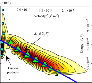
Figure 16. (a) Differential current distribution of all droplets (main and fast) versus mass/charge (m/q = 2ξu ⁻²) and energy. The symbols mark the points of maximal probability at fixed ξ for main and fast droplets. The lines correspond with linear fits to the main drop symbols (solid line) and to the path of minimum slope to the peak (ridge, dash dot). The inset magnifies the fast drop region. (b) Separate m/q distributions for the main and fast drops.

The combination of the high velocity and the low energy of the fast drops yields a rather small m/q, which we shall see is associated with drop sizes considerably below the jet diameter. These fast drops must accordingly be either the product of Coulomb fissions of larger drops, or satellite drops produced during the jet breakup process. It is possible to reject the second of these two alternatives, as satellites form typically in numbers comparable to the main drops (i.e. figure 5 of Tang & Gomez Reference Tang and Gomez1994), and carry much less overall charge. In contrast, the daughters from one Coulombic explosion of a conducting drop are numerous, and collectively may carry as much as half the original parent drop charge (Richardson, Pigg & Hightower Reference Richardson, Pigg and Hightower1989). The Coulombic fission of all primary (much larger) electrosprayed drops can be visualized in some splendid images reported by Yang et al. (Reference Yang, Duan, Li and Deng2014, figure 4d), where a periodic jet breakup was electrically forced with an external harmonic perturbation.

There is finally a spurious step associated with the retrograde signal previously discussed which we include in the analysis of the data but whose characteristics are irrelevant. The parameters for the three step functions are collected in table 6.

4.8. Determination of jet characteristics

Figure 15(a) represents the differential drop current distribution constructed based on the fits inferred at all available energies for the main and fast droplets. At each energy we have an error function (4.7), whose derivative with respect to the horizontal variable u ⁻² is

(4.8)\begin{equation}\textrm{d}I(\xi ,u) = \frac{{b(\xi )}}{{\sqrt {2{\rm \pi}} \,\textrm{d}(\xi )}}\textrm{exp}\left[ { - \frac{{{{({u^2} - c{{(\xi )}^2})}^2}}}{{2\,\textrm{d}{{(\xi )}^2}}}} \right]{u^4}{\xi ^2}\,\textrm{d}\frac{1}{\xi }\,\textrm{d}\frac{1}{{{u^2}}}.\end{equation}

The maximum of this distribution for given ξ provides an approximately linear relation ${\xi ^{ - 1}}({u^{ - 2}})$ (triangles in figure 15a), whose slope and y intercept yield the jet breakup velocity and potential according to (4.2c).

An alternative representation of this current distribution in terms of the variables ξ and $m/q = 2\xi /{u^2}$ is also of interest (4.9), and is depicted in figure 16

(4.9) \begin{equation}\textrm{d}I(\xi ,m/q) = \dfrac{{\sqrt {\dfrac{2}{\rm \pi}} b(\xi )}}{{d(\xi ){{\left( {\dfrac{m}{q}} \right)}^2}}}\textrm{exp}\left[ { - \dfrac{{{{\left( {2\xi {{\left( {\dfrac{m}{q}} \right)}^{ - 1}} - c{{(\xi )}^2}} \right)}^2}}}{{\; 2d{{(\xi )}^2}}}} \right]\xi \,\textrm{d}\xi \,\textrm{d}\dfrac{m}{q}.\end{equation}

The position of the ridge in this figure falls on an approximately straight line, as expected from (4.6). Its y intercept gives V_j = 1205 V, while its slope $m = U_j^2/2$ yields U_j = 444 m s⁻¹ (^b line in table 7). To illuminate the level of ambiguity of this determination two alternative calculations of U_j, V_j and ΔV are included in lines c and d of table 7, based on the two additional regression lines included in figures 15(a) and 16(a).

Table 7. Jet breakup parameters (velocity, potential, diameter, irreversible voltage drop (4.1) and associated temperature rise) inferred from the distribution of drop velocity and energy, and propulsive parameters for the spray calculated using (4.10) to (4.13). The jet potential and velocity have been extracted from the ridge on figure 16(a).

^aMass flow rate and thrust have been scaled by 1.21 to compensate for the disparity between I_TOF (max corrected nA) and emitted current. This correction assumes that all of the missing signal is species independent.

^bRidge of figure 16(a).

^cContinuous line in figure 16(a).

^dRegression line in figure 15(a).

The fraction of mass flow rate and thrust at each energy can be calculated by numerical integration of (4.9) as described in (4.10) and (4.11). The overall drop flow rate and thrust are obtained by adding the partial values across all energies. This method can yield the mass fractions for each species

(4.10)\begin{gather}\dot{m} = \; \mathop \sum \limits_i \int {\frac{m}{q}\,\textrm{d}I({\xi _i},m/q)} ,\end{gather}

(4.11)\begin{gather}T = \sum\limits_i {\int {u\frac{m}{q}\,\textrm{d}I({\xi _i},m/q)} } = \sum\limits_i {\int {{{\left( {2{\xi_i}\frac{m}{q}} \right)}^{1/2}}\,\textrm{d}I({\xi _i},m/q)} } .\end{gather}

Ion properties are calculated using their nominal m/q, with b_i and c_i instead of dI and u, respectively. Therefore $\dot{m} = \sum\nolimits_i {(m/q){b_i}} ;\;T = \sum\nolimits_i {{c_i}(m/q){b_i}}$. In any case, all contributions other than those from the main drops are negligible in mass flow and fairly small in thrust. The overall flow rate and thrust are obtained by adding the contribution from each species.

Specific impulse and polydispersity efficiency are defined as

(4.12)\begin{gather}{I_{sp}} = \frac{T}{{\dot{m}g}},\end{gather}

(4.13)\begin{gather}{\eta _{poly}} = \frac{{{\textstyle{1 \over 2}}\dot{m}{{({I_{sp}}g)}^2}}}{{{V_o}{I_e}}}.\end{gather}

If one were to replace V_o by V_e in (4.13) one would obtain the thruster efficiency. In our case, where the difference between V_e and V_o is not measurable, η_poly = η_thruster. More fundamentally, η_poly is defined as the ratio between the power actually consumed to achieve a given mass flow rate $\dot{m}$ and thrust T to the minimal power required to obtain them. This minimal power is attained for a monodisperse plume containing a unique q/m, when one readily sees that ${P_{min}} = {T^2}/(2\dot{m})$. It is clear that the presence of ions and fast drops decreases this efficiency because they consume a power proportional to their current yet achieve almost no thrust.

4.9. On the distribution of drop velocities

We believe the measured distributions of velocities and energies for particles of given m/q are real rather than a by-product of our finite energy resolution. The question is, what causes these widths? The observed distribution of ξ measured for dimer ions b ₂(ξ) could be due either to (a) the distribution of V_j resulting from temporal variability of the position of the breakup point, or rather (b) to other sources of randomness, especially the fact that the breakup process is not periodic, so energy conservation is not strictly applicable. We shall here assume hypothetically scenario (a) to show that it is incompatible with our data. In that hypothesis, the measured ion energy distribution would coincide with the distribution of jet breakup potentials

(4.14)\begin{equation}P({V_j}) = {b_2}({V_j}).\end{equation}

From this distribution one may now infer the distribution of drop energies and velocities, since the jet velocity U_j and electrical potential V_j are linked by the equation of energy conservation (4.1), which applies down to the jet breakup point. Therefore, unless there is an additional source of particle velocity fluctuation, the probability distributions of U_j and V_j should be simply related. Accordingly, we write the particle velocity from (4.6) as

(4.15)\begin{equation}{u^2} = [{V_o} + {V_j}(1/\alpha - 1)]2{q_j}/{m_j}.\end{equation}

This equation predicts indeed a variation in u ² as a result of variations in V_j. However, the sensitivity of u ² to changes in V_j is proportional to (α ⁻¹ − 1) and vanishes when α = 1. According to (4.6), this condition corresponds also to a unique particle energy, ξ = V_o. Therefore, if the main source of particle velocity dispersion at fixed energy were the dispersion in jet breakup potential, there would be no velocity dispersion at the mean energy. In our measurements (see section C of supplementary material for higher energy resolution), however, drops with this special energy exhibit a velocity spread comparable to that of drops with other energies. From this we cannot but conclude that the mechanism responsible for the observed spread in velocity in approximately monoenergetic drops is not just due to the variation in U_j and V_j associated with the randomness in the position of the jet breakup point. A more probable explanation for the observed spread in velocities is that it is substantially due to unsteadiness in the process of drop production. It would therefore persist even if the breakup point were exactly fixed. If the jet was periodically excited close to the most unstable frequency for drop production, such that drops of a fixed volume would be delivered in each period, all drops would also acquire the same energy. However, since drops of widely different sizes are produced in each pinching of the jet, with different intervals between successive pinchings, the breakup process is capable of injecting different energies and velocities even into identical drops, depending on the sizes of the neighbouring drops produced either before or after. In other words, energy is conserved in our unsteady processes only on the average, but not for each individual drop. Therefore, understanding the observed velocity, size or charge distributions of the drops will require modelling the unsteady breakup process.

The special situation encountered at ξ = V_o of a velocity insensitive to fluctuations in V_j makes intuitive sense, as V_o may be viewed as the total energy available to accelerate first the jet from zero initial kinetic energy, and then to further accelerate the drops to their final energy. Drops having an energy equal to V_o also have the same charge/mass as the jet: q/m = I/(ρQ), and are accelerated to exactly the same final velocity whether they are in jet form or drop form. Therefore, their final velocity cannot be affected by changes in the position of the breakup point

4.10. Comparison of observed and expected jet parameters

4.10.1. Jet breakup characteristics

Comparisons are made in table 8 between our results for EMI-FAP and those of Gamero-Castaño (Reference Gamero-Castaño2008) for the different IL EMI-Im and for numerous electrolytes of tributyl phosphate (TBP). The table relies on the following definitions:

(4.16a–c)\begin{equation}r_G^6 = \rho {\varepsilon _0}{Q^3}/(\gamma K);\quad {L^9} = {\rho ^2}{Q^5}{\varepsilon _0}/(K{\gamma ^2});\quad L/{r_G} = {[\rho KQ/(\gamma {\varepsilon _0})]^{1/18}},\end{equation}

and shows that the two ILs operate in comparable regimes. The characteristic length r_G originally used by Gañán-Calvo (Reference Gañán-Calvo1997) has been shown by Gamero-Castaño & Hruby (Reference Gamero-Castaño and Hruby2002) to provide a suitable scale for the jet breakup diameter in their measurements with electrolytes of tributylphosphate. The value of r_G also provides a length scale that collapses into very similar shapes a number of numerical calculations of cone jets (Gamero-Castaño Reference Gamero-Castaño2010; Gamero-Castaño & Magnani Reference Gamero-Castaño and Magnani2018). The alternative scale L in (4.16b) is suggested by the asymptotic form proposed by Gañan-Calvo for the jet diameter d_j as a function of the axial distance z to the apex of the cone: D ⁴z ^1/2 = C (i.e. (19) of Gañán-Calvo et al. Reference Gañán-Calvo, López-Herrera, Herrada, Ramos and Montanero2018), where the constant C naturally defines the new length scale as L ^9/2 = C. Note from (4.16c) that the lengths r_G and L have comparable numerical values because they are related through a very small (1/18) power of the dimensionless parameter ρKQ/($\gamma\varepsilon_0$), which is never particularly large or small.

Table 8. Characteristics of our jets compared with prior work.

^aPresent study. ^bGamero-Castaño (Reference Gamero-Castaño2008). ^cGamero-Castaño and Hruby (Reference Gamero-Castaño and Hruby2002). ^dEquation (4.16a). ^eEquation (4.16b). ^fEquation (4.17d). ^gEquation (4.17a–c) with $\varepsilon$ = 8.9, α(8.9) = 5.33, β(8.9) = 1.92.

4.10.2. Irreversible voltage drop

Given the potential of the jet at the meniscus base and its mean value at the breakup point, the irreversible potential drop may be determined from (4.1) using the mean jet velocity. This quantity is presented in table 7 and turns out to have an unphysical negative value. The corresponding jet temperature change, if substantial, would have drastic effects on fluid properties. For instance, while glycerol electrolytes have insufficient conductivity to evaporate ions, they do nevertheless produce ions when run at sufficiently high voltage (Cook Reference Cook1986). More remarkably, Fedkiw & Lozano (Reference Fedkiw and Lozano2009) have shown that the singularly viscous and poorly conducting IL 1-butyl-3-methylimidazolium iodide is able to operate in the purely ionic regime of emission. A simple explanation for these anomalies is that dissipation increases the tip temperature sufficiently to produce local electrical conductivities adequate for ion evaporation. The temperature change due to dissipative losses may be obtained from the emission current, the mass flow rate and the assumption that the unknown heat capacity of EMI-FAP is similar to that of the related ionic liquid 1-butyl-3-methylimidazolium tris(pentafluoroethyl) trifluorophosphate (BMI-FAP) (c_p = 1193 J kg⁻¹ K⁻¹ (Safarov et al. Reference Safarov, Lesch, Suleymanli, Aliyev, Shahverdiyev, Hassel and Abdulagatov2017)) as $\Delta T = \; (\Delta VI/{c_p}\dot{m}) ={-} 1.06\;\textrm{C}$, by assuming that all of the electrical energy dissipated is transformed into heat, and that there are no losses to the environment. These unphysical negative losses are nevertheless small compared with the uncertainties in our experiment, including a 120 V discretization of the energy, and typical drop energy distributions widths of several 100 V. Furthermore, as seen in table 7, our determination of the jet breakup potential involves errors of tens of Volts. This limited precision precludes determining reliably the temperature rise in our relatively thick jets, but should be adequate for more dissipative jets.

Gamero-Castaño (Reference Gamero-Castaño2008) reports jet breakup velocities U_j and voltages V_j, for the IL EMI-Im. The irreversible voltage drop calculated from his table 1 as ${V_e} - {V_j} - {\textstyle{1 \over 2}}\rho QU_j^2/I$ gives values very close to zero, evidently because V_j was obtained directly from the measured ion energy, but U_j was inferred indirectly by assuming a reversible acceleration. Gamero Castaño (Reference Gamero-Castaño2010) has investigated numerous electrolytes of three organic solvents of relatively low viscosity, under a variety of electrical conductivities and flow rates. He concluded that

(4.17a–d)\begin{align}\Delta V = {V^\ast }F(\varepsilon );\quad {V^\ast } = {\gamma ^{2/3}}/({K^{1/3}}\varepsilon _0^{1/6}{\rho ^{1/6}});\quad F(\varepsilon ) = [\alpha (\varepsilon ) + \beta (\varepsilon )/Re];\quad Re = {(\rho {\varepsilon _0}\gamma^2/K)^{1/3}}/\mu ,\end{align}

where $\varepsilon_0$ is the dielectric constant of the liquid, and the range of Re ⁻¹ covered varied from approximately 0.15 to 5. The quantities α and β in (4.17c) take values of order unity for the range of dielectric constants investigated, which varied from approximately 8.9 to 111. The values of 1/Re and V* for EMI-Im and EMI-FAP at room temperature are collected in table 8. The dielectric constants for these two ILs are unknown, but should be comparable to that of tributyl phosphate, for which Gamero-Castaño reports α(8.9) = 5.33, β(8.9) = 1.92. Equation (4.17) applied to the ILs would predict ΔV = 997 V and 575 V for EMI-FAP and EMI-Im, respectively. These values are vastly larger than what we have measured here, suggesting that (4.17) does not apply to EMI-FAP. A possible reason for this discrepancy is that our Re is well below the range studied by Gamero-Castaño (Reference Gamero-Castaño2010). An investigation with electrolytes of more viscous fluids would help clarify the matter. Another possibility is that perhaps neat ILs behave differently from electrolytes containing modest salt concentrations.

Our conclusion on the inapplicability of (4.17) to ILs is confirmed by a recent study on EMI-Im (Gamero-Castaño & Cisquella-Serra Reference Gamero-Castaño and Cisquella-Serra2021) reporting independently measured jet breakup velocities and potentials at the centre of the beam. From their tables we infer ΔV values from 40 to 180 V, one order of magnitude below the extrapolation from (4.17). In spite of a considerable scatter in these data, ΔV increases markedly with Q, in sharp contrast with the prior striking observation on the independence of ΔV on Q for electrolytes of organic solvents. In summary, both ILs exhibit a much smaller level of energy dissipation than suggested by prior work on electrolytes of low viscosity solvents.

4.10.3. Emission potentials

Using the jet velocity from table 7 and assuming it to be constant, the emission potential of the various drops can be calculated. This is done by subtracting the energy gained in the jet from the final energy of the particle. Figure 17(a) reproduces the data of figure 16(a) in terms of the new variables. It is visually clear on figure 17(a) that for the main drops (m/q~ > 0.0004 kg C⁻¹) at higher mass over charge ratios the emission potential has a higher spread. One also sees that the fast drops (m/q~ < 0.0004 kg C⁻¹) display a wider range of emission potentials than the main drops. The source of this effect is discussed below.

Figure 17. (a) Data of figure 16 with the y axis changed from ξ into ${V_E} = \xi - {\textstyle{1 \over 2}}(m/q)U_J^2$. (b) Distribution of emission potential V_E at five intervals of mass over charge whose centre and width are marked by the vertical lines and error bars in (a). The emission energy of the dimer ion is also displayed. The FWHM are approximately 440, 180, 220, 260, 370, 300 V following the order of the legend.

4.10.4. Diameter of the drops

While we can infer the breakup radius of the jet ${R_j} = {\{ Q/({\rm \pi} {U_j})\} ^{1/2}}$, we lack direct information on the radii of the drops. Approximate drop size information may nevertheless be obtained from the fact that a drop of radius R may at most carry Rayleigh's limiting charge ${q_R} = 8{\rm \pi} {({\varepsilon _0}\gamma {R^3})^{1/2}}$, where γ is the surface tension of the liquid forming the drop (35.3 dyn cm⁻¹ at room temperature for EMI-FAP, table 1) and $\varepsilon_0$ is the electrical permittivity of vacuum. Therefore, Rayleigh's charge ratio η_R is always less than unity

(4.18)\begin{equation}{\eta _R} = \frac{q}{{8{\rm \pi} \sqrt {{\varepsilon _0}\gamma {R^3}} }} \le 1.\end{equation}

We may accordingly write m/q in terms of R and η_R only, or alternatively express the drop radius in terms of the experimental quantity m/q as

(4.19)\begin{equation}R = {(m/q)^{2/3}}{(36\eta _R^2{\varepsilon _0}\gamma /{\rho ^2})^{1/3}}.\end{equation}

Therefore, except for an ambiguity in the factor of order unity $\eta _R^{2/3}$, the m/q information included in figure 16 can be converted into drop radius information. This is done for the drop diameter in the upper horizontal scales of figure 16 for the representative cases where the Rayleigh ratio is either 1 or ½.

When η_R = 1 the fast drops have a mean diameter of 10.7 nm. The associated surface electric field is 1.7 V nm⁻¹, sufficient to evaporate ions. However, fast drops cannot be the source of most of the ions observed because the total ion current exceeds threefold that of fast drops. Nevertheless, the Coulomb explosions yielding these fast drops involve the formation of transient jets on the main drops having diameters about half the diameter of the fast drops (5 nm). These jets would naturally also support electric fields adequate for ions to evaporate, not only from their tip, but predominantly from their neck region, with associated currents that could be up to half the current originally carried by main drops. Furthermore, because the main drops would originally carry most of the jet current, while ions represent approximately ¼ of the total, it is certainly possible that most ions would be released from exploding main drops. This scenario would demand the fission of a substantial percentage of the main drops, a situation that has been previously demonstrated by Yang et al. (Reference Yang, Duan, Li and Deng2014), even for 100 % of the main drops. Their outstanding images confirm also that the jet produced during the transient fission of the main drops is approximately half the diameter of the daughter drops, and much smaller than the main jet diameter. The notion that ions are evaporated from fissioning main drops slightly downstream from the breakup point is also compatible with the observation that ion energies (~1130 V) are modestly but clearly below the jet breakup potential (~1205 V). Figure 17(b) provides further evidence for this fissioning. The FWHM of the emission potential for relatively large drops having mass/charge = 0.0067 kg C⁻¹ is more than twice that at 0.001 kg C⁻¹. This wider distribution is expected if most or all of these large drops had undergone a Coulombic explosion within a range of positions, ultimately causing a higher spread of emission potentials. An additional indication of the high probability that the large drops would explode is given by the ratio of electrostatic to capillary stresses on the jet, ${\varPsi _j} = \textrm{ }I_j^2d_j^3/(64{Q^2}\gamma {\varepsilon _0})$, which for our jet takes a value 0.806, relatively close to unity. Let us now assume that the average drop radius R_D is a factor η_D larger than the jet radius, and that the charge over mass of the average drop is the same as that of the jet. Then, the ratio of electrostatic stresses to capillary stress on the average drop is ${\varPsi _D} = {\varPsi _j}(2\eta _D^3/9)$. Taking η_D to be 1.89, as in Lord Rayleigh's inviscid breakup of a neutral jet, results in ${\varPsi _D} = 1.5{\varPsi _j}$, which for our jet gives ${\varPsi _D} = 1.21$. Our drops are therefore estimated to be on the average charged above the Rayleigh limit, so it makes sense that a substantial fraction of them would undergo either Coulomb explosions or ion evaporation.