


1. Introduction
Recent studies following a large eddy simulation (LES) of a Mach 0.9 round jet (Brès et al. Reference Brès, Jaunet, Rallic, Jordan, Colonius and Lele2015) have clearly identified a system of instability waves that are not the same as the well-known Kelvin–Helmholtz (K–H) waves (Schmidt et al. Reference Schmidt, Towne, Colonius, Cavalieri, Jordan and Brès2017; Towne et al. Reference Towne, Cavalieri, Jordan, Colonius, Schmidt, Jaunet and Brès2017; Brès et al. Reference Brès, Jordan, Jaunet, Rallic, Cavalieri, Towne, Lele, Colonius and Schmidt2018). These, referred to as ‘trapped waves’ or ‘guided waves’, are predicted by additional solutions of spatial stability analysis of a free cylindrical shear layer, apart from the solution for the K–H waves. While the reader may consult the cited references as well as Edgington-Mitchell et al. (Reference Edgington-Mitchell, Jaunet, Jordan, Towne, Soria and Honnery2018), Mancinelli et al. (Reference Mancinelli, Jaunet, Jordan and Towne2019) and Bogey (Reference Bogey2021) for details of such analyses, a brief summary is provided in the following.
The analyses involve linearized inviscid solutions based on the system of equations for spatial stability of a cylindrical vortex sheet; see, e.g. Michalke (Reference Michalke1984). Michalke (Reference Michalke1970) first noted a second ‘mode’ in the solutions apart from the K–H mode. While the latter mode involved pressure amplitude maxima in the shear layer, the second mode had a maximum on the jet centreline with a node in the radial profile. Michalke commented that ‘mode II has never been found experimentally’ and therefore may not be ‘compatible with a realistic jet’. Tam & Hu (Reference Tam and Hu1989) later conducted a detailed analysis and identified two sub-branches of the second mode – one with supersonic and the other with subsonic propagation speeds (see also Morris Reference Morris2010). Focusing on supersonic jet flows, Tam and Hu noted that the waves due to the second mode were confined within the jet and that part of the subsonic waves could also propagate upstream in a narrow frequency band. Tam later studied the role of these guided upstream propagating waves in various flow resonance phenomena, such as screeching jets (Shen & Tam Reference Shen and Tam2002), impinging jets (Tam & Ahuja Reference Tam and Ahuja1990) and jets grazing over a plate (Tam & Chandramouli Reference Tam and Chandramouli2020).
The existence of the guided or trapped waves and their role in flow-acoustic resonance phenomena received a flurry of attention in the late 2010s. As stated already, Towne et al. (Reference Towne, Cavalieri, Jordan, Colonius, Schmidt, Jaunet and Brès2017) noted these waves in the LES results of Brès et al. (Reference Brès, Jaunet, Rallic, Jordan, Colonius and Lele2015) for a Mach 0.90 jet. Towne et al.'s stability analysis showed that both upstream and downstream propagating waves could exist in the Mach number range of 0.82 to 1. Combined with end conditions imposed by the nozzle and the contracting potential core, they showed that these oppositely propagating waves could set up resonances with resultant pressure fluctuations characterized by distinct spectral peaks. Brief experiments accompanying their study confirmed the existence of such spectral peaks in the vicinity of the jet. A recent numerical and analytical work by Bogey (Reference Bogey2021) predicted the occurrence of such p’-spectral peaks within and outside of the jet, over a wider range of jet Mach numbers (0.6–2.0), which generally agreed with the experimental data obtained earlier in the present study (Zaman & Fagan Reference Zaman and Fagan2019).
The occurrence of the p’-spectral peaks in the vicinity of high subsonic jets came as a surprising revelation. These basically went undetected and unrecognized over decades of experimental studies on jet noise and flow instability. These disappear in the far acoustic field and thus went unnoticed in jet noise experiments. They also went undetected in jet instability experiments, apparently because the K–H waves persist farther and dominate the flow field. Furthermore, the latter experiments are mostly conducted in incompressible jets, whereas these waves seem to occur only in high-speed, compressible jets. It is also possible that probe interference, such as with hot-wire anemometry, alters the trapped waves and renders them difficult to discern.
The near-field spectral peaks were nonetheless encountered in at least one previous experiment. Suzuki & Colonius (Reference Suzuki and Colonius2006) noted them in a Mach 0.9 jet when a few of the microphones in a ‘phased array’ exhibited such spectral peaks. They thought these were spurious and possibly related to facility resonances. They explored the connection of these peaks to upstream duct modes, the result of which was inconclusive, and narrated their observations in an appendix to the paper.
Only limited experimental studies have been conducted to date on the subject. A notable one is that of Edgington-Mitchell et al. (Reference Edgington-Mitchell, Jaunet, Jordan, Towne, Soria and Honnery2018), who performed particle image velocimetry measurements in low supersonic jets undergoing the ‘A1’ and ‘A2’ stages of screech at nozzle pressure ratios of 2.10 and 2.25, respectively. The existence of the upstream propagating waves was demonstrated at both conditions. Whereas the K–H waves were modulated by the shock cells and had amplitude maxima in the shear layers, the latter waves had a distinctly different distribution, having maxima on the jet centreline and radial shapes as predicted by the second-mode solution of the stability analysis. Edgington-Mitchell et al. (Reference Edgington-Mitchell, Wang, Nogueira, Schmidt, Jaunet, Duke, Jordan and Towne2021) further studied various wavelike structures in a supersonic jet experimentally as well as analytically. They detected both upstream and downstream propagating guided waves in addition to the K–H waves and discussed their relevance to the screech phenomenon. Another impressive study is that of Mancinelli et al. (Reference Mancinelli, Jaunet, Jordan and Towne2019), who investigated the occurrence of the A1 and A2 screech stages and the associated jump in frequency with variation of the jet Mach number. The upstream propagating waves predicted by stability analysis, when considered in the feedback loop, were shown to yield screech tones that agreed very well with their measurements.
Clearly, there should be more than an academic interest to understanding the near-field pressure fluctuations due to the trapped waves. They are an integral part of the jet shear layer instability that in turn dictates the initial development of the jet. Even though these waves are not readily detectable in the far field, it stands to reason that computational fluid dynamics and aeroacoustics codes must account for them for accurate prediction of jet noise. Another possible relevance of the trapped waves could be in jet–surface interaction and, therefore, in propulsion or airframe noise. A plate when placed near a nozzle often yields resonant tones that might have a connection to these waves (Tam & Ahuja Reference Tam and Ahuja1990; Jordan et al. Reference Jordan, Jaunet, Towne, Cavalieri, Colonius, Schmidt and Agarwal2018; Tam & Chandramouli Reference Tam and Chandramouli2020). However, this last aspect has not been adequately explored in our study and will not be addressed further in this paper.
The present experimental study aims at gaining a better understanding of the characteristics of the near-exit unsteady pressure fluctuations and their prevalence with various nozzles. Following Towne et al. (Reference Towne, Cavalieri, Jordan, Colonius, Schmidt, Jaunet and Brès2017), such fluctuations will be simply referred to as ‘trapped waves’ and the corresponding spectral peaks in the pressure signal as ‘trapped wave spectral peaks’. A host of questions could be raised. Does the efflux boundary layer (BL) state (laminar vs. turbulent) of the jet affect them? As with K–H waves, do their frequencies scale with the thickness of the BL? Can they be observed on a typical ‘Ffowcs Williams–Hawkings’ surface used for far-field noise prediction? Is there a harmonic relationship among the successive peaks? Do they occur in non-axisymmetric jets? A link between the trapped waves and screech tones was apparent from our preliminary experiments (Zaman & Fagan Reference Zaman and Fagan2019); with increasing jet Mach number, it appeared that certain trapped wave spectral peaks amplified and turned into the screech tones. Is there a common thread in the mechanisms of the trapped waves and screech tones leading to such an observation? We attempt to address these questions in the present study. The measurements are relatively simple; using moveable microphones the spectra of the pressure fluctuations are measured outside of the jet for varying streamwise and radial distances as well as for varying jet Mach number. Round nozzles of different diameters as well as rectangular nozzles of different aspect ratios are explored. Since a large parameter-space is covered, only key findings are described, with observations mainly from an experimentalist's vantage point without any analytical effort; however, some connections with the analytical and numerical efforts of others are made where relevant. Preliminary results of the experiment were presented in a conference paper (Zaman & Fagan Reference Zaman and Fagan2020), as well as in the document cited above (Zaman & Fagan Reference Zaman and Fagan2019).
2. Experimental facility
The experiments are conducted in an open jet facility at the NASA Glenn Research Center. Compressed air passes through a 30 inch diameter plenum before exhausting through the nozzle into the ambient of the test chamber; all dimensions are given in inches. An interested reader may find further description of the facility in earlier publications, e.g. Zaman (Reference Zaman1999) and Zaman et al. (Reference Zaman, Fagan, Bridges and Brown2015). The pressure fluctuation spectra are measured by microphones (1/4″, B&K 4135) placed suitably near the nozzle exit. Limited far-field noise spectra are also measured with fixed microphones. Data acquisition is done using a National Instruments analogue-to-digital card and LabVIEW software. Spectral analysis is done typically over a 0–50 kHz range with a bandwidth of 50 Hz, using a data rate of 100 kHz and a 50 kHz low-pass filter. For the larger rectangular nozzles a 0–25 kHz analysis range (25 Hz bandwidth) is used. The data are often shown over a shorter range so that the spectral peaks are illustrated adequately.
Figure 1 shows pictures of various nozzle configurations. All nozzles are convergent. The round one in figure 1(a) is the ‘SMC000’ case (where ‘SMC’ stands for ‘small metallic chevron’ nozzle and extension ‘000’ denotes the baseline case without the chevrons); it will be referred to simply as ‘SMC’ in the following. It is attached to the plenum chamber through adapters with smooth, converging interior contours. This round nozzle with an exit diameter of 2″ has been used previously in several experimental as well as numerical studies; Zaman (Reference Zaman2019) cites a few such works. For round nozzles, distances are non-dimensionalized by the diameter D. For rectangular nozzles, the length scale used for non-dimensionalization is either the equivalent diameter based on area (also denoted as D) or the narrow dimension (h), as indicated.
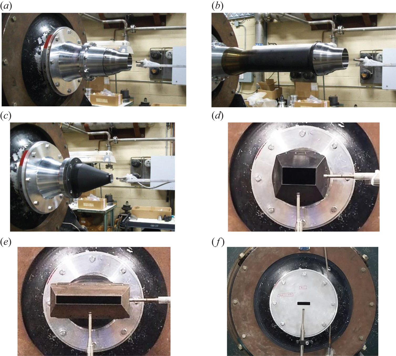
Figure 1. Nozzle configurations. (a) D = 2″ (‘SMC’) nozzle, (b) SMC nozzle with a 12″ long upstream pipe, (c) D = 1″ nozzle, (d) 2 : 1 rectangular nozzle, (e) 8 : 1 rectangular nozzle, (f) 4 : 1 orifice nozzle.
The configuration shown in figure 1(b) involves the SMC nozzle with a 12″ long upstream pipe. It has been shown to generate a fully turbulent exit BL, whereas without the pipe the nozzle has a ‘nominally laminar’ BL; this is discussed with the results. Figure 1(c) shows a 1″ diameter round nozzle; a 0.58″ diameter round nozzle is also used, which is not shown for brevity. While the exit BLs for the smaller nozzles have not been measured, they are also likely to be nominally laminar. Figures 1(d) and 1(e) show the rectangular nozzles ‘R2’ and ‘R8’ with aspect ratios of 2 and 8, respectively; not shown is the ‘R4’ nozzle with an aspect ratio of 4. These ‘R’ nozzles have been used in previous experiments (also referred to as ‘NA2Z’, ‘NA4Z’ and ‘NA8Z’ in earlier publications); electronic files of their profiles can be found in e.g. Zaman (Reference Zaman2012). These three nozzles have the same equivalent diameter based on the exit area, D = 2.12″. The narrow dimensions (h) for the three nozzles are 1.328″, 0.939″ and 0.664″, respectively. Further descriptions and exit BL data for these nozzles can be found in the cited reference. A few other rectangular nozzles are also used to document screech frequency characteristics. These include a set of rectangular orifices with aspect ratios ranging from 1 to 16; figure 1(f) shows one of them. These have an equivalent diameter D = 1″ and are denoted as the rectangular orifice (RO) cases. Small rectangular nozzles, denoted as ‘R_sm’ cases, with D = 0.58″ are also used for screech frequency documentation. The RO and R_sm nozzles were originally used for studying the spreading characteristics of non-axisymmetric jets (Zaman Reference Zaman1999).
The ‘jet Mach number’ MJ is used as an independent variable. It is defined based on the nozzle pressure ratio, i.e. the ratio of the plenum pressure, p 0, and the ambient pressure, pa, and given by  ${M_J} = {(({({p_0}/{p_a})^{(\gamma - 1)/\gamma }} - 1)(2/\gamma - 1))^{1/2}}$, where γ is the ratio of specific heats for air. Note that in supersonic conditions, MJ is fictitious and represents the Mach number had the flow expanded fully. Similarly, UJ represents the jet velocity had the flow expanded fully. All data reported are for cold flows, i.e. with the total temperature the same everywhere as in the ambient. It should be noted that there is a flow rate limitation for the facility (approximately 4 lb s−1) to avoid excessive recirculation within the test chamber. This limited the maximum Mach number that could be covered with the larger R nozzles to approximately MJ = 1.4. With the smaller nozzles, higher values of MJ could be covered.
3. Results and discussion
3.1. Round nozzle data
Pressure fluctuation spectra measured near the exit of the SMC nozzle are shown in figure 2(a) for varying streamwise distances (x). The distances are non-dimensionalized by the nozzle diameter (2″) and the coordinate origin is located at the centre of the nozzle exit. The ordinate pertains to the trace at the bottom (x = −0.5) and successive traces are staggered by 10 dB. The radial locations for the eight traces follow a typical Ffowcs Williams–Hawkings surface (Brès et al. Reference Brès, Jordan, Jaunet, Rallic, Cavalieri, Towne, Lele, Colonius and Schmidt2018; Liu et al. Reference Liu, Corrigan, Johnson and Ramamurti2019) and are indicated in the figure legends. A series of peaks mark the spectra, especially near the nozzle exit. These are similar to those reported by Towne et al. (Reference Towne, Cavalieri, Jordan, Colonius, Schmidt, Jaunet and Brès2017) and Suzuki & Colonius (Reference Suzuki and Colonius2006). Away from the exit, the spectral peaks get buried under the broadband turbulence, apparently when the microphone encounters some flow. In figure 2(b) corresponding data are shown for a fixed x but for varying r. When the microphone is too close to the jet (r = 0.6), it encounters flow resulting in a broadband peak, in this case centred around 12 kHz. The spectral peaks are seen to diminish in amplitude with increasing radial distance.

Figure 2. Pressure spectra near the exit of the SMC (D = 2″) nozzle; MJ = 0.91. (a) Varying x (on a Ffowcs Williams–Hawkings surface, see text), (b) varying r at fixed x = 0.2. (Distances normalized by D.)
The fact that the spectral peaks are detected in the vicinity of the jet's edge may suggest that these are ‘hydrodynamic’, i.e. footprints of events within the jet. However, the data at x = −0.5 (figure 2a), as well as limited surveys in the near field (Fagan & Zaman Reference Fagan and Zaman2020), showed that they occurred unabated upstream of the nozzle's exit. This likely implies that the spectral peaks involve significant propagative (acoustic) components. In fact, Bogey's (Reference Bogey2021) study shows that these peaks are detectable in the far acoustic field in the upstream direction. Further evidence can be seen from the present data in figure 3(b).
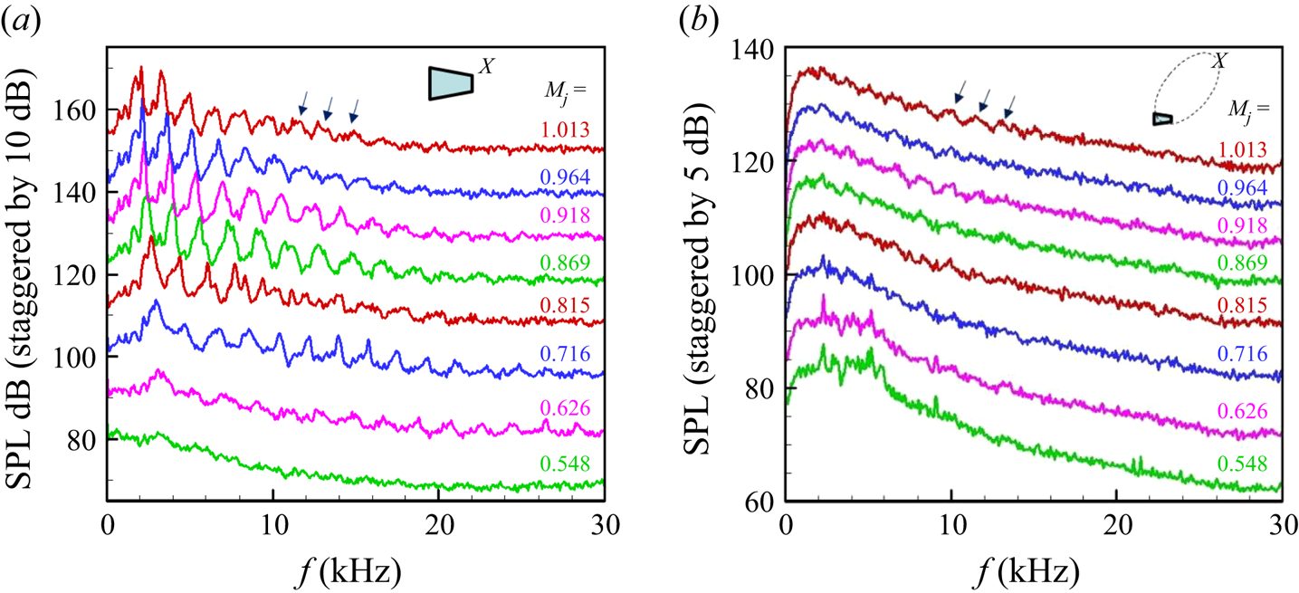
Figure 3. Pressure spectra near and far from the SMC nozzle with varying MJ. (a) Near-exit at x = 0.2, r = 0.75, (b) 25D away from the exit at 60° polar location relative to jet axis.
Corresponding data for varying jet Mach number (MJ) at a point near the nozzle exit (x = 0.2, r = 0.75) are shown in figure 3(a). The trapped wave spectral peaks are not quite visible at the lowest MJ (=0.548), but they become prominent at higher MJ, the frequency of a given peak decreasing with increasing MJ. Such behaviour was also noted by Suzuki & Colonius (Reference Suzuki and Colonius2006), leading to the inference that these peaks do not follow a Strouhal number scaling (if the Strouhal number based on nozzle diameter remained constant, the frequencies would increase with increasing MJ). In figure 3(b), corresponding sound pressure level spectra in the ‘far field’ are shown; the microphone location is 25D from the jet exit and at a polar angle of 60° relative to the jet axis (the location is shown schematically, with inserts in some figures to aid the reader). The trapped wave spectral peaks are known to be undetectable in the far-field noise spectra. Here, some undulations (marked by the arrows), especially at higher MJ conditions, correspond to the trapped wave peaks in figure 3(a). Thus, as noted in the previous paragraph, these peaks may not be simply hydrodynamic and involve significant propagative (acoustic) components. For the data in figure 3(b), one should note that the experimental arrangement is not anechoic and there are some uncovered reflecting surfaces in the vicinity of the nozzle (e.g. the probe traversing mechanism, flanges, etc.) that might have an impact on the measured spectra.
Effect of initial BL state and nozzle diameter
Figure 4(a) shows pairs of spectral data at three values of MJ. These data are for the SMC nozzle, with one set taken with the upstream pipe (figure 1b) and the other without the pipe (figure 1a). Through hot-wire measurements it was found that the nozzle with the pipe involved a fully turbulent exit BL, whereas the case without the pipe involved a ‘nominally laminar’ BL; details of the BL state with varying MJ for the SMC nozzle can be found in the reference Zaman (Reference Zaman2019). In essence, the nominally laminar case involves mean velocity profiles similar to a textbook ‘Blasius profile’. The turbulent case, on the other hand, involves a slow decay of the mean velocity as the nozzle wall is approached, until a sharp drop occurs near the wall. Turbulent fluctuations in the latter case penetrate far from the wall. A set of mean velocity and turbulence profiles at MJ = 0.825, shown in figure 4(b), exhibit these differences. The legend ‘SMC+’ represents the turbulent case (with upstream pipe). The momentum thickness in the turbulent case is approximately three times larger than that in the nominally laminar case.

Figure 4. Data for the SMC nozzle with and without the upstream pipe; SMC+ denotes the pipe case (see figure 1b). (a) Pressure spectra at x = 0.2 and r = 0.75 at three different MJ; the three pairs are staggered successively by 10 dB, last number in legend is overall sound pressure level (OASPL) (dB). (b) Exit boundary layer profiles at MJ = 0.825.
The nearly congruent traces at each MJ in figure 4(a) indicate that the trapped waves are not influenced by the exit BL characteristics. It is noted that in the LES work of Brès et al. (Reference Brès, Jordan, Jaunet, Rallic, Cavalieri, Towne, Lele, Colonius and Schmidt2018), the trapped wave peaks were also observed in both initially laminar and turbulent BL cases. It is also apparent that the trapped wave spectral peaks do not scale on the exit BL thickness for a given BL state (laminar or turbulent); BL thickness decreases with increasing MJ, so a Strouhal number based on the thickness would not remain constant and would decrease rapidly with increasing MJ. The frequency scaling is discussed further in the following sections.
One other point is noteworthy. Figure 4(a) includes a set of data at a supersonic condition where screech has ensued (represented by the tall peak in the spectra, which manifests as an audible tone). The progression of the spectral peaks with increasing MJ suggests that one of the trapped wave peaks has turned into the screech component. This point is also addressed further in the following. Note that the ‘trapped wave’ spectral peaks are quite sharp and, with the resolution of analysis, are as much as 15 dB above the broadband levels. However, none of them emitted perceptible audible tones as far as the authors could tell. On the other hand, the screech component at MJ = 1.09, standing approximately 40 dB above the broadband levels, was loud and clearly audible.
Figure 5(a) shows data from the 1″ diameter nozzle with varying x. Very similar trends are noted, as seen in figure 2(a), for the 2″ nozzle, except that the frequencies of the peaks are higher. The same comment can be made for the radial variation of the spectra shown in figure 5(b) when compared with the data in figure 2(b). Likewise, a similar trend is observed for jet Mach number variation, shown in figure 6(a). In figure 6(b), data for the 1″ diameter nozzle are shown in the supersonic regime. In the range MJ ≥ 1.083 there is screech. With increasing MJ the screech frequency decreases and there is a ‘stage jump’ around MJ = 1.2. An inspection again reveals a connection. It is as if the screech component locks on to one of the trapped wave spectral peaks. With increasing MJ, it locks on to the third peak (e.g. at MJ = 1.117) and after the stage jump it locks on to the second peak. Throughout the entire MJ range, the frequency of an individual peak in a given stage decreases with increasing MJ. The link with screech is addressed further in the following.

Figure 5. Pressure spectra near the exit of D = 1″ nozzle for MJ = 0.91. (a) Varying x at fixed r = 0.75, (b) varying r at fixed x = 0.2.

Figure 6. Pressure spectra for D = 1″ jet with varying MJ; x = 0.2, r = 0.75. (a) Low Mach number range, (b) supersonic range.
Frequency scaling and harmonic relationships
Data for an even smaller nozzle (D = 0.58″) were also obtained, and a consistent increase in the frequencies of the trapped wave peaks was noted with decreasing nozzle diameter. This is examined in figure 7, where data for all three nozzles are plotted as a function of Strouhal number based on the diameter. Two sets of data are shown for MJ = 0.92 and 1.01, as examples, in figures 7(a) and 7(b), respectively (in the supersonic regime, as stated before, UJ represents the ‘ideal’ jet velocity had the flow expanded fully). The trapped wave spectral peaks are found to be essentially congruent for the three nozzles with different diameters. Scrutiny also reveals that the spectral peaks are not direct (integral) harmonics. For example, the first three peaks for MJ = 0.91 occur at Strouhal numbers 0.377, 0.624 and 0.879; those for MJ = 1.01 occur at 0.345, 0.576 and 0.808. However, one finds that the ratio of the second and first numbers (0.624/0.377) is approximately 5/3, while that of the third and the second numbers (0.879/0.624) is approximately 7/5. The same ratios hold true at the higher MJ. See further discussion at the end of this subsection.

Figure 7. Pressure spectra for the three round nozzles shown as a function of Strouhal number based on diameter; x = 0.2, r = 0.75. (a) MJ ≈ 0.91, (b) MJ ≈ 1.01.
The Strouhal numbers of the four tallest peaks in each spectra (usually the four from the left at low frequencies) are plotted in figure 8. The symbol size (and shape) are varied according to the amplitude; circles represent the highest while the square, diamond and delta shapes represent the lower amplitudes in decreasing order. Note also that red, blue and green symbols represent the 2″, 1″ and 0.58″ nozzles, respectively. A clear trend emerges. The trapped wave spectral peaks follow distinct branches. Generally, the amplitudes are the highest at the lowest branch and decrease at the upper branches. However, screech, representing the tallest peak in the supersonic regime, often locks on to the peaks in the upper branches. Screech is seen to blend in with the family of curves quite well.

Figure 8. Strouhal numbers of the four tallest spectral peaks, cross-plotted from data similar to those in figure 3(a) for round nozzles of three diameters. Equation for fundamental (fit 1) given in the text; Curves 2, 3 and 4 are 5/3, 7/3 and 9/3 harmonics, respectively.
Also shown in figure 8 are four data points from the paper of Suzuki & Colonius (Reference Suzuki and Colonius2006). Their data (denoted ‘SC’) agree well with the current data. From the phased array measurements, they furthermore determined the mode shapes associated with each of the four data points, as indicated in the legend. It appears, therefore, that the branches representing the fundamental and the 2nd harmonic (1st and 3rd branches) are of the axisymmetric (m = 0) shape, while the 1st and 3rd harmonics (2nd and 4th branches) are of the helical (m = 1) shape. It is noted, however, that Bogey's (Reference Bogey2021) analysis attributes successively different mode shapes to the four spectral peaks. With the instrumentation of the current experiment this could not be examined further.
It is apparent that the trapped wave spectral peaks follow a Strouhal number scaling after all (based on nozzle diameter). However, the Strouhal number is not a constant and it is a distinct function of MJ in each of the four branches (figure 8). The results on exit BL effect (figure 4) and for nozzles of different diameters (figures 7 and 8) strongly suggest that the spectral peaks do not scale with the initial shear layer (efflux BL) thickness. Had the ratio of the thickness to diameter remained constant for all nozzles, scaling on the diameter would be equivalent to scaling on the BL thickness. Although it has not been measured, that ratio is unlikely to be the same for all three nozzles. Furthermore, there is the stark contrast in BL thickness in figure 4(a) (a factor of three difference in momentum thickness) that has practically no effect on the spectral peaks. In figure 8, if the data were non-dimensionalized by exit BL thickness instead of diameter they would not fall on a single curve for each branch. Thus, it is safe to infer that the trapped wave spectral peaks do not scale on initial shear layer thickness, contrasting the characteristics of K–H waves.
The data in figure 8 provide an engineering correlation for prediction of the trapped wave frequencies for round nozzles. For a given diameter, the frequencies are represented by empirical curves fitted through the data. In the earlier reports (Zaman & Fagan Reference Zaman and Fagan2019, Reference Zaman and Fagan2020) curves of the shape  $St = M_J^{ - A} + B$ were fitted where St was the Strouhal number (ordinate in figure 8). Those curves significantly deviated from the data in the supersonic regime. A better fit for the fundamental was obtained with the equation
  ${St = (1/M_J^2 - 1)/14 + (1/{M_J} - 1)/2 + 0.35}$. This is shown by ‘fit 1’ in figure 8. With reference to the discussion regarding an integral relationship among the frequencies of the spectral peaks in figure 7, and with the peaks denoted as f 1, f 2, f 3, etc., with increasing frequency, the following relationships were apparent:
  ${f_2} = (5/3){f_1},\textrm{ }{f_3} = (7/5)f_2 = (7/3){f_1}$, etc. That is,
  ${f_n} = ((2n + 1)/3){f_1}$. Curves 2, 3 and 4 are plotted accordingly by simply multiplying the fundamental by the respective factors. The matchings of these curves with the data are excellent.
As indicated in the Introduction, there have been several recent numerical and analytical studies on the trapped wave phenomenon, following the seminal studies of e.g. Towne et al. (Reference Towne, Cavalieri, Jordan, Colonius, Schmidt, Jaunet and Brès2017). Let us compare the predictions of Towne et al. (Reference Towne, Cavalieri, Jordan, Colonius, Schmidt, Jaunet and Brès2017) and Bogey (Reference Bogey2021) for the spectral peak frequencies with the current data. As an example, consider the Strouhal numbers of the first five peaks at MJ = 0.9. From ‘fit 1’ and harmonics (figure 8), these are found to be 0.42, 0.70, 0.99, 1.27 and 1.55. Towne et al. compared analytical predictions with spectra obtained from the LES data of Brès et al. (Reference Brès, Jaunet, Rallic, Jordan, Colonius and Lele2015) as well as their own experimental results. Their spectral peaks, although not as sharp as seen in the present experiment, were nonetheless unambiguous. The predictions yielded bands of frequencies around each of the spectral peaks (figure 10 of Towne et al.). The centre frequencies of these bands for the first five peaks corresponded to Strouhal numbers of 0.39, 0.61, 0.91, 1.21 and 1.52. The numbers are quite close to the five values from the present experiment. Bogey (Reference Bogey2021), on the other hand, performed LES for a variety of conditions. For a case comparable to our experiment, at MJ = 0.9, the LES data yielded spectral shapes for near-field pressure fluctuations very similar to the present data. His stability analysis of a cylindrical vortex sheet also yielded resonant frequencies agreeing well with the LES spectral data. The Strouhal numbers for the first five peaks (his figure 25c) turned out to be 0.42, 0.71, 1.00, 1.27 and 1.56. These numbers are amazingly close to our experimental values.
The fractional relationship  $({f_n} = ((2n + 1)/3){f_1})$ for the spectral peak frequencies, discussed in the foregoing, is peculiar. One is tempted to think that there might be a ‘mysterious’ true fundamental at 1/3 the value of ‘fit 1’ (then, the successive curves would be simply odd harmonics of that fundamental). However, scrutiny does not reveal the existence of such spectral peaks in any of the plots; the reader may inspect figures 2–7. Was the observed fractional harmonic relationship a mere coincidence? The excellent agreement of the correlation curves with the data (figure 8, see also figure 9), as well as the numerical and analytical predictions of Bogey (Reference Bogey2021) in particular, strongly suggest that such harmonic relationships are indeed in play. However, none of the previous studies noted this behaviour, much less attempted an analytical explanation.
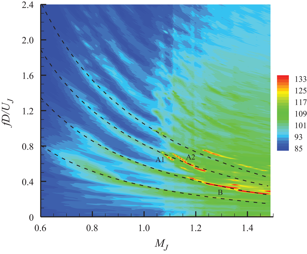
Figure 9. Contour plot of SPL spectral amplitudes (in dB) taken with the SMC nozzle at small intervals of MJ (microphone at x = 0.2, r = 0.75). The main screech stages are identified. The four dashed curves are the same empirical fits as in figure 8.
Linkage to screech tones
The apparent linkage of the trapped wave spectral peaks with screech tones was further explored by obtaining data with the SMC nozzle at small increments in MJ. The result is shown by the contour plot of spectral amplitude in figure 9. The plot is based on 47 spectral traces from the fixed near-field microphone. On the left, in the subsonic regime, the branches of trapped waves can be seen clearly; the dashed lines are the empirical fits discussed with figure 8. In the supersonic regime, screech tones are represented by the regions of high amplitudes (red). Well-known screech stages (A1, A2 and B) are captured within the MJ range covered and marked in the plot (Norum Reference Norum1984; Raman Reference Raman1999). (Note that in the earlier conference paper, Zaman & Fagan (Reference Zaman and Fagan2020), these stages were mislabelled; this is corrected in figure 9.) The upper bands of deep red on the right are due to the harmonic of stage B. It becomes apparent that the A1 and A2 stages approximately match the general continuation of the third branch of the trapped waves. Even though these two stages, having the jump in between, do not match exactly, they are in close vicinity of the branch 3 curve. Stage B, on the other hand, matches branch 2 quite well. Overall, that screech seems to occur as a continuation of the trapped wave branches is almost unmistakable. This may lead one to speculate that the morphology of screech and the trapped wave spectral peaks rests on similar foundations. This indeed becomes particularly apparent from the works of Mancinelli et al. (Reference Mancinelli, Jaunet, Jordan and Towne2019) and Bogey (Reference Bogey2021). Screech stages A1 and A2 are successfully predicted by invoking the guided upstream propagating waves in these analyses (see also Edgington-Mitchell et al. Reference Edgington-Mitchell, Jaunet, Jordan, Towne, Soria and Honnery2018, Reference Edgington-Mitchell, Wang, Nogueira, Schmidt, Jaunet, Duke, Jordan and Towne2021). The same upstream propagating wave, confined within the core of the jet and interacting with the downstream propagating guided wave, also explained the trapped wave spectral peaks in subsonic flows (Towne et al. Reference Towne, Cavalieri, Jordan, Colonius, Schmidt, Jaunet and Brès2017). Thus, the common thread in the mechanisms is the upstream propagating guided wave completing the feedback in either phenomenon. Note that this notion of the screech mechanism is different from traditional views that assume acoustic waves outside of the jet to be responsible for completing the feedback loop; the cited references provide detailed discussions of these differences in the concepts. A possible link between the trapped waves and screech is discussed further with the rectangular nozzle data in the following section.
3.2. Rectangular nozzle data
Observations on major axis vs. minor axis
The presence of the trapped waves in rectangular jets was demonstrated in our earlier reports (Zaman & Fagan Reference Zaman and Fagan2019, Reference Zaman and Fagan2020). As with round nozzles, they occurred above a certain MJ, and the frequencies of individual spectral peaks decreased with increasing MJ. The number of spectral peaks depended on the side of the nozzle where the microphone was placed. The latter behaviour is illustrated in figure 10. The pressure fluctuation spectra on the major axis (short edge) is compared with that on the minor axis (long edge) for the R2 nozzle in figure 10(a). The microphone locations are shown by the schematic insets; the locations are h/2 from the nozzle's lip in all cases, where h is the narrow dimension of the nozzle. It is seen that peaks occur less frequently on the minor axis. The first dominant peak (fundamental) is the same on both edges but only the third and fifth seen on the major axis coincide with the second and third seen on the minor axis; at higher frequencies the amplitudes are small and there is increasing randomness in such matching. However, it is apparent that the peaks seen on the minor axis approximately coincide with every other peak seen on the major axis.
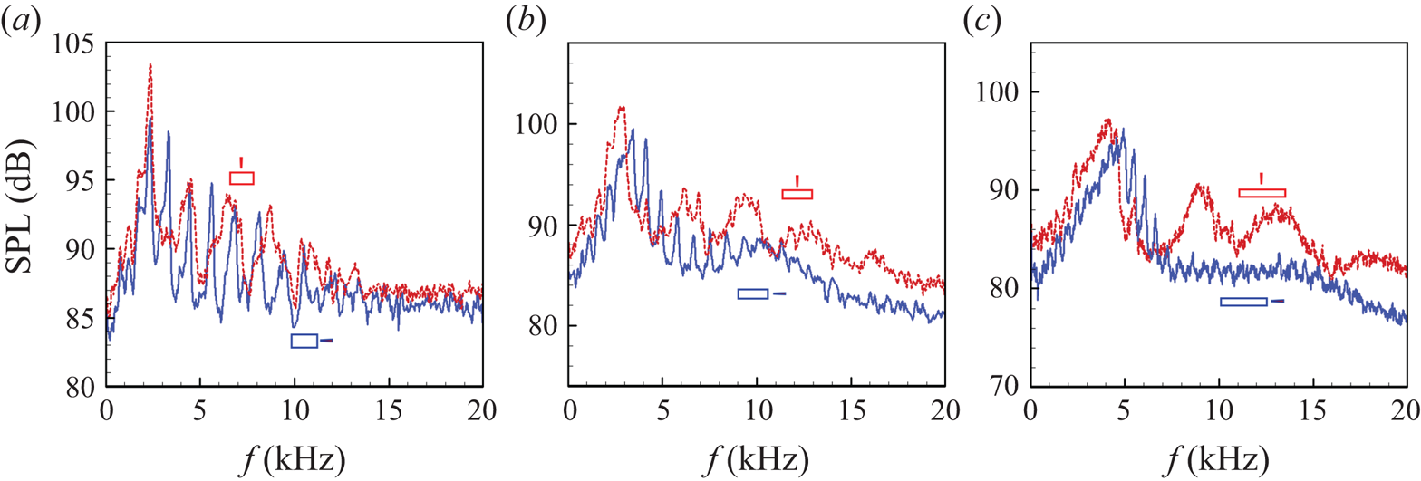
Figure 10. Pressure fluctuation spectra at x = 0.5″, MJ = 0.91, with the microphone on the major axis (blue solid line) and the minor axis (red dashed line). Panel (a) shows data for the R2 nozzle, (b) shows the R4 nozzle, (c) shows the R8 nozzle; the microphone is placed approximately at h/2 away from the nozzle lip, where h is the narrow dimension of the respective nozzle. Microphone locations are schematically shown by the insets.
Similar comparisons for the R4 and R8 nozzles are made in figures 10(b) and 10(c), respectively. In both cases, the spectral peaks are tightly packed on the major axis, while on the minor axis the peaks are dispersed and not as sharp. An inspection suggests that the number of peaks on the minor axis for the R4 case is approximately four times less than that on the major axis. Similarly, that ratio for the R8 nozzle is approximately 8. Therefore, the number of peaks on the minor axis is less than that seen on the major axis by a factor roughly equal to the aspect ratio of the nozzle. It appears that a lateral resonance in the major axis direction, whose wavelength is dictated by the major dimension, modulates the fundamental when observed from the minor axis location. Similarly, a resonance with wavelength dictated by the minor dimension modulates the fundamental when observed from the major axis location. It will be shown in the following section that the fundamental, for the larger aspect ratio (AR) nozzles, is dictated by the minor dimension of the nozzle.
Spectral evolution with Mach number
Detailed spectral evolution with varying MJ in a ‘waterfall’ format is shown in figure 11 for the R2 nozzle. For clarity, the results are divided into two groups for lower and higher Mach number regimes, shown in the bottom and top rows, respectively. Data for the minor axis location are shown in the left column while those for major axis location are shown in the right column. The value of MJ is indicated on the right of each spectral trace. A visual perspective on the evolution of the trapped wave spectral peaks can be obtained from these data.
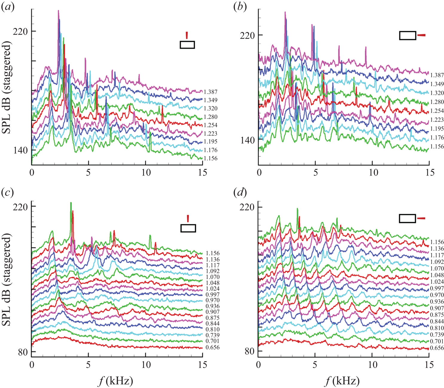
Figure 11. Near-field pressure fluctuation spectra for the R2 nozzle. The left column data for microphone on the minor axis; the right column data for microphone on the major axis; the bottom row shows the lower MJ range; and the top row shows the higher MJ range. In each figure, successive traces are staggered by 5 dB (minor tick spacing on ordinate); the ordinate scale pertains to trace at the bottom. Values of MJ for each trace are indicated along the side. Microphone at x = 0.5″ and 0.66″ from nozzle lip in all cases.
Consider the minor axis data on the lower left of figure 11. The trapped wave fundamental (dominant peak at the lowest frequency) is barely visible at the lowest MJ. With increasing MJ it becomes prominent and persists into the supersonic regime while its frequency continuously decreases. Noticeable higher-frequency peaks appear around MJ = 0.81. Here, the higher-frequency peaks appear to be (integral) harmonics of the fundamental. Recall that for a round nozzle the higher frequency peaks were 5/3, 7/3, 9/3 … multiples of the fundamental.
As with the round nozzles, the transition of the spectral peaks into screech can also be seen from the minor axis data (figure 11 left). At approximately MJ = 1.14, the second trapped wave peak (first harmonic) is suddenly amplified into a sharp spike with accompanying tone (in this instance at 3.64 kHz). The plot in the upper row captures the subsequent evolution of this screech tone. Its frequency continues to decrease with increasing MJ, here, at a rate faster than that of the fundamental. At high MJ, the harmonic relationship with the trapped wave fundamental is lost. At MJ = 1.14, the fundamental and screech components occur at 1.82 and 3.64 kHz, respectively (harmonics). At MJ = 1.28, for example, these two peaks occur at 1.63 and 2.81 kHz, respectively (not harmonics); this is discussed further shortly.
The data for the major axis location on the right of figure 11 show a similar spectral evolution. The fundamental trapped wave peaks remain the same as seen on the minor axis. However, the number of peaks is greater. A comparison at a given MJ at subsonic conditions shows that for each pair of adjacent peaks on the minor axis, there is a third in the middle of the corresponding data on the major axis.
Spectral evolution for the R4 nozzle are similarly shown in figure 12. Here, the trends are somewhat obscured. The trapped wave fundamental (f 1) on the minor axis (left column) becomes clear at approximately MJ = 0.85. As with the R2 nozzle, the fundamental persists all the way to the highest MJ ( = 1.39) covered in the experiment. The higher harmonics of the fundamental are not quite clear. Screech ensues at MJ = 1.05 with a relatively high frequency and jumps to a lower frequency at slightly higher MJ (1.12). Subsequently, the cluster of screech peaks at even higher MJ appears near the first harmonic (2f 1). These trends are scrutinized further in the following. On the right of figure 12, at the major axis location, the trapped wave peaks are clearer in the subsonic regime. A band of those peaks appear at higher frequencies and this band moves to the left with increasing MJ until screech appears.

Figure 12. Near-field pressure fluctuation spectra for the R4 nozzle, shown similarly as in figure 11.
Corresponding data for the R8 case are shown in figure 13. The trends in the evolution are again obscured. (A contour plot, as in figure 9, did not show the trends any better for any of the R nozzles, thus the ‘waterfall’ format is used.) Nonetheless, similar observations can be made as with the R4 data in figure 12. The fundamental becomes apparent at approximately MJ = 0.9 and persists into the supersonic regime. As with the R4 case, screech starts around MJ = 1.05, then jumps to a lower frequency at MJ = 1.105 before the screech peaks are subsequently seen to be clustered around the first harmonic (2f 1) for the rest of the MJ range.

Figure 13. Near-field pressure fluctuation spectra for the R8 nozzle, shown similarly as in figure 11.
More on the link with screech tones
The trapped wave fundamental and its relationship to screech tones are examined in figure 14. First, the fundamental Strouhal number variation is shown in figure 14(a). Data for the R2, R4, R8 and round case are shown as a function of MJ. The curve for the round nozzle is the same as ‘fit 1’ in figure 8. As discussed for figures 12 and 13, the spectral peaks for the R4 and R8 nozzles are obscured, and best guess results for the fundamental are shown. It is found that the fundamental for the R2 case is close to the curve for the round case (recall that D is the equivalent diameter in the rectangular cases). The Strouhal number (fD/UJ) for the higher aspect-ratio nozzles is higher especially in the low MJ range.
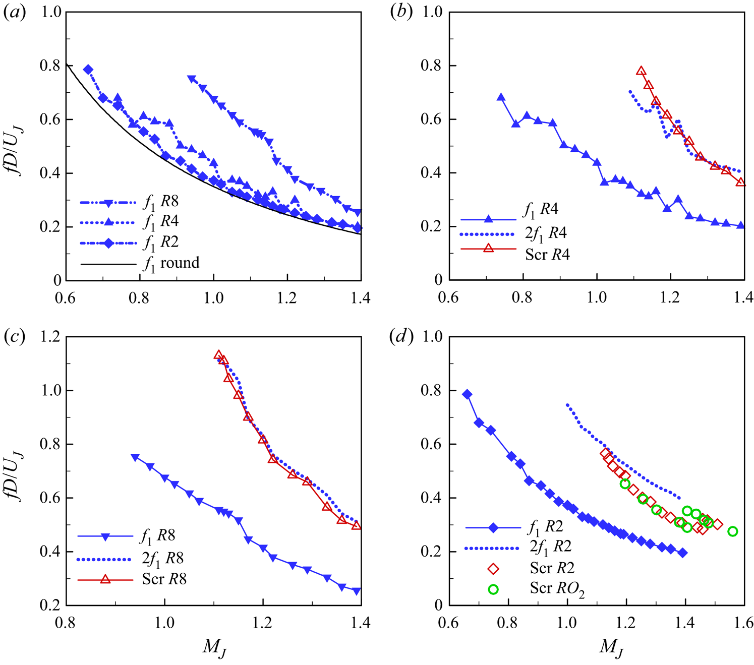
Figure 14. Strouhal numbers of fundamental trapped wave peak and screech. (a) Fundamental (f 1) for R2, R4 and R8 nozzles compared with the round case. (b) Fundamental and screech for R4 case. (c) Fundamental and screech for R8 case. (d) Fundamental for R2 case compared with screech for R2 and RO 2 cases.
In figures 14(b) and 14(c), screech frequency variation is compared with that of the fundamental (f 1) for the R4 and R8 nozzles, respectively. Also shown is the profile for the first harmonic (=f 1*2) with the dotted lines. There is some ambiguity in reading f 1 and screech data manually from the spectra; however, it is apparent that the screech frequency is approximately the same as the first harmonic in the entire supersonic regime. Reading the data for the R2 nozzle was less ambiguous, but the trends are different (figure 14d). In this case, as noted with figure 11, screech starts at the first harmonic (2f 1), but with increasing MJ its frequency deviates from 2f 1. The aspect ratio 2 case, however, undergoes a stage jump in screech. Such a stage jump with smaller AR nozzles was noted earlier (e.g. Zaman Reference Zaman1999). It is seen to occur with the 2 : 1 orifice nozzle around MJ = 1.4 (figure 14d). The Mach number range covered for the larger R2 nozzle was limited up to approximately MJ = 1.4 because of facility limitations (discussed in section II). However, using some precautions a few additional data at MJ > 1.4 could be obtained that confirmed the stage jump with the R2 case around MJ = 1.45. Interestingly, the curve for the first harmonic (2f 1) tends to approach the screech frequency after the stage jump. That is, with increasing MJ the screech frequency deviates from 2f 1 but returns to 2f 1 after the stage jump. We make some further comments on this issue in the last paragraph of this section, but first screech tones with various rectangular nozzles and scaling of their frequencies are examined.
Screech with rectangular nozzles
In addition to the R2, R4 and R8 cases, further data on screech tone were acquired with the RO nozzles that covered a wide range of aspect ratio. This effort was prompted partly by a confusion in rectangular nozzle screech data in the literature (M. Samimy, personal communication; see also Esfahani, Webb & Samimy Reference Esfahani, Webb and Samimy2021). Part of the confusion arose because in an earlier work with small nozzles (Zaman Reference Zaman1999), ca*MJ, instead of UJ, was used as a velocity scale to calculate the Strouhal number; here, ca is the speed of sound in the ambient and UJ is the ‘fully expanded’ jet velocity. The data in Esfahani et al. (Reference Esfahani, Webb and Samimy2021), as in many other works on the subject, are presented as Strouhal numbers based on the equivalent diameter (D) and UJ. This format is used in the following. It should be noted that ca*MJ and UJ are uniquely related, and use of the former results in a 10–20 % lower value of the Strouhal number depending on MJ, but the data trends remain the same. However, the appropriateness of the length scale (D) may be in question, and this is examined in the following discussion.
The screech data for the R2, R4 and R8 nozzles are shown in figure 15(a). Note that the two high frequency data for the R4 and R8 nozzles around MJ = 1.07 (figures 12 and 13) are ignored so that the trends could be shown with sufficient ordinate resolution. Figure 15(a) also includes screech data taken with the orifice nozzles of the same AR values (2, 4 and 8) (data for the 2 : 1 case are the same as in figure 14d). A few observations can be made. First, as with round nozzles, the screech Strouhal number for all cases decreases with increasing MJ. Second, screech ensues at a somewhat lower Mach number (MJ ≈ 1.1) for the R nozzles compared with that for the smaller RO cases (MJ ≈ 1.2). The reason for this remains unclear; however, there are obvious geometrical differences, such as a large reflecting surface with the RO cases (figure 1f) that has been known to affect screech amplitude (e.g. Raman Reference Raman1999). Third, the non-dimensional frequencies fall on a single curve, for a given AR, regardless of the size difference between the R and RO cases (D = 2.12″ vs. 1″, respectively). Thus, it is apparent that screech frequency is dictated simply by the (convergent) nozzle exit geometry, and details of the upstream geometry have little impact. Note that a stage jump is noted with the smallest AR case; with RO 2 it occurs around MJ = 1.4 while with R2 it occurs at a somewhat higher MJ (1.45). Finally, and most importantly, it becomes clear that the aspect ratio factors into the data trends; fD/UJ at a given MJ is increasingly large with increasing AR. The diameter D is not the right length scale to dictate the rectangular nozzle screech frequency. Instead, the small dimension h dictates the frequency in most cases, as demonstrated in the following.

Figure 15. Screech data for various rectangular cases. (a) R2, R4 and R8 nozzle data together with data for corresponding orifice cases, RO 2, RO 4 and RO 8; (b) square orifice data compared with round nozzle data.
As stated before, in order to complete an understanding of the effect of AR on rectangular nozzle screech behaviour, further data were taken with the RO nozzles. Figure 15(b) is included to show the behaviour in the limiting case of a square nozzle. Data for the AR = 1 (square, RO 1) case are compared with round nozzle (Rdsm) data. The latter data, shown by the solid lines, are reproduced from Zaman (Reference Zaman1999). The well-known screech stages for the round case are indicated in the figure; see Norum (Reference Norum1984) and Raman (Reference Raman1999). It is apparent that the square nozzle behaves quite similarly, involving multiple stages, some of which seemingly coincide with the circular jet data. As discussed in the next figure, the staging behaviour becomes less prevalent with increasing AR.
Data for several rectangular cases are shown in figure 16, with frequency non-dimensionalized by the small dimension h. The data sets include an RO case with AR = 16, a small AR = 3 nozzle (R_sm_3) reproduced from Zaman (Reference Zaman1999), and AR = 5 nozzle data obtained in the same jet facility by Raman (Reference Raman1997). As evident from figure 15(a), if the equivalent diameter (D) were used for non-dimensionalization, these data would scatter all over the plot. Non-dimensionalization by h collapses most of the data. The square nozzle data, involving multiple stages, are excluded in the comparison in figure 16 to avoid clutter. Note that the data from Raman (Reference Raman1997) are reproduced by digitization of the published graph, and an average curve is shown by the blue line. It is worth mentioning that Raman's data for the AR = 5 nozzle reproduced well when obtained in a different facility (Panda, Raman & Zaman Reference Panda, Raman and Zaman1997). The small AR = 3 case data were also spot checked in the current experiment. We note here that several of the nozzles in the comparison of Esfahani et al. (Reference Esfahani, Webb and Samimy2021) are convergent–divergent, with which screech frequencies may scale somewhat differently depending on the flow regime. All nozzles in figure 16 are convergent and involve under-expanded flows.

Figure 16. Screech data for R2, R4 and R8 nozzle compared with orifice and other rectangular cases; the ordinate is a non-dimensional frequency based on the narrow dimension of the nozzle.
It is clear from figure 16 that apart from the smallest AR cases, all other data involving aspect ratios 4, 5, 8 and 16 are clustered into one curve. Note the expanded ordinate scale compared with that in figure 15(a). Even for the AR = 3 (R_sm_3) case, the data for the most part fall into this cluster. Thus, for aspect ratios greater than approximately 3, the narrow dimension is the right length scale dictating the screech frequency. When the aspect ratio is smaller than 3, the flow does not behave as ‘two-dimensional’ and the data trend deviates; there are three-dimensional effects and occurrence of screech stage jumps. Within the MJ range covered in figure 16, stage jumps occur for cases with AR = 3 or less. Furthermore, the data (together with AR = 1 case in figure 15b) illustrate that the stage jump shifts to higher MJ with increasing AR.
Going back to the issue of the link between the trapped wave peaks and screech, it is apparent that if screech frequency scales with h, so will the fundamental frequency, since the two are related harmonically (figure 14). This is indeed found to be the case from the data of figure 14(a) for the R4 and R8 cases when plotted on a Sth (=fh/UJ) vs MJ format. The fundamentals for the two nozzles are essentially congruent on such a plot. A fitted curve through all data in the format  $S{t_h} = M_J^{ - A} + B$ is given by the coefficients (A, B = 0.3584, −0.8049); this is not shown for brevity but can be inferred from figure 14(a), bearing in mind that D/h = sqrt(AR*4/π). It should be obvious that this correlation applies only to the larger aspect-ratio nozzles and not to cases with AR < 3. Note that obtaining detailed spectral evolution data involved significant time and effort and could be achieved only for the R nozzles, hence the correlation is based on data for only the R4 and R8 nozzles. Furthermore, as stated before, there was subjectivity in reading the fundamental frequencies. Thus, the fitted curve should be considered only as an approximation. Importantly, it is plausible that the same analysis with the upstream propagating guided waves, as done for round jets in the various cited works, might also predict the trapped wave fundamental and screech for the rectangular nozzles. However, these comments are based solely on observation of the experimental data, and to the authors’ knowledge no analysis has been done for the rectangular nozzles yet. Further experimentation, analysis and numerical simulation would be needed for a full understanding of the link between the trapped wave spectral peaks and screech tones.
4. Conclusions
Near the nozzle exit and around the edge of high-speed jets, unsteady pressure fluctuations are observed that manifest as a series of peaks in the spectrum. It is remarkable that these spectral peaks have gone undetected in decades of jet noise and jet instability experiments. This is because they do not appear in the far field and hence were not noticed in far-field noise measurements. Similarly, they went unnoticed in instability experiments because those experiments mostly focused on incompressible flows, whereas the phenomenon is apparently characteristic of compressible jets. The spectral peaks are the footprints of ‘trapped waves’ and their resonance within the potential core of the jet, as revealed by recent research based on LES and analytical studies. In this experimental study, the characteristics of the spectral peaks are explored for a set of round nozzles of different diameters, as well as a set of rectangular nozzles of different aspect ratios. In all cases, the frequency of the spectral peaks is found to decrease with increasing jet Mach number. For the round nozzles, it is shown that the spectral peaks remain unaffected by the exit BL state and thickness. The frequencies are found to scale on the jet diameter. The Strouhal numbers, based on the diameter for all round nozzles, are found to follow distinct branches of a family of curves when plotted as a function of MJ. It is apparent that successive peaks (branches) are harmonics bearing a frequency relationship to the fundamental as 1, 5/3, 7/3, 9/3, and so on. Correlation equations are provided.
The trapped wave spectral peaks are also observed with all rectangular nozzles. However, the frequencies of the peaks depend on the observation location. More tightly packed spectral peaks are observed on the major axis (short edge), while the peaks are dispersed on the minor axis (long edge) location. The ratio of the number of peaks on the major axis to that on the minor axis is found to be approximately equal to the aspect ratio of the nozzle.
With increasing jet Mach number the onset of screech is noted to occur as a continuation of the trapped wave branches. It is as though one of the trapped wave spectral peaks gets amplified and turns into the screech component. For round nozzles, it is the third branch of the trapped waves (7/3 harmonic) that first turns into screech. With further increase in MJ there is a stage jump when the screech component matches the continuation of the second branch (5/3 harmonic) of the trapped waves. With the 4 : 1 and 8 : 1 rectangular nozzles, even though there is some ambiguity in identifying the spectral peaks, screech frequency follows the first (integral) harmonic. With the 2 : 1 rectangular case, there is a stage jump complicating the data trends; however, overall, the screech frequency is also seen to follow the first harmonic of the trapped wave fundamental.
Recent numerical results by other researchers on the round jet near-field pressure fluctuation spectra agreed very well with our experimental data. The experimental observations on the connection of screech with the trapped waves also appear to be supported by the analytical and numerical studies by others. The common element is the upstream propagating guided (trapped) waves. These waves resonate with downstream propagating waves, explaining the trapped wave spectral peaks in the subsonic regime. Apparently the same upstream propagating waves also complete the feedback in at least some of the screech cases in the supersonic regime.
Acknowledgements
The first author wishes to thank Dr A. Towne of the University of Michigan for a discussion of the topic at the AIAA/CEAS Aeroacoustics Meeting in May 2019 that inspired the present experimental effort, and Professor C. Tam of Florida State University, whose analytical work inspired the experiments with the rectangular nozzles. Special thanks are due to our colleague Dr C. Miller for pointing out the harmonic relationship among the spectral peaks for the round nozzles, as well as coming up with the equation for empirical fit through the data.
Funding
This work is supported by NASA's Commercial Supersonic Technologies (CST) and Transformational Tools and Technologies (TTT) Projects.
Declaration of interests
The authors report no conflict of interest.


