


1. Introduction
The analysis of turbulent flows is not a trivial task as they have a chaotic and unpredictable nature. This task becomes increasingly difficult at high Reynolds numbers ( $Re$). Although the imposition of a surface in a turbulent flow is of practical importance, it generates further challenges as it leads to the existence of inhomogeneity, anisotropy and a wide range of spatiotemporal scales. Within the near-wall region of wall-bounded flows, relevant statistical quantities attain a maximum such as the mean viscous stress, flatness, turbulence kinetic energy, premultiplied spectra, turbulence production and viscous dissipation. This shows how dynamic and intermittent the near-wall region is. Additionally, essential turbulence quantities of canonical wall-bounded flows (pipe flow, channel flow and zero pressure gradient (ZPG) turbulent boundary layer (TBL)) such as vorticity (
 $\boldsymbol {\omega }$) are generated at the wall (Batchelor Reference Batchelor1967; Morton Reference Morton1984). Moreover, the large velocity gradients and the rate at which these quantities evolve near the wall significantly influence the intensification and dampening of vorticity within this region (Davidson Reference Davidson2004).
Understanding the near-wall region ( $y^+ \lesssim 100$) of wall-bounded turbulent flows has progressed substantially during the last century in several aspects, such as its statistical universality, organisation and self-sustaining mechanisms. Nevertheless, the nonlinearities that sustain near-wall turbulence still require a more profound understanding (McKeon Reference McKeon2017; Bae, Lozano-Durán & McKeon Reference Bae, Lozano-Durán and McKeon2021) especially for unconstrained flows at high Reynolds numbers (Panton Reference Panton2001). In that context, the present paper examines the precursors of rare backflow (BF) events and shows that these rare events are related to a nonlinear vortex autogeneration occurring near the wall.
Due to the nature of pipe flows, a cylindrical coordinate system has been adopted in this study, where  $x$,
$x$,  $r$ and
  $\theta$ represent the streamwise, radial and azimuthal directions. The wall-normal direction is defined as
  $y=R-r$, where
  $R$ is the pipe radius. Here
  $U_x$,
  $U_y=-U_r$ and
  $U_\theta$ are the streamwise, wall-normal and azimuthal velocity components. Similarly, the fluctuating velocity components are
  $u_x$,
  $u_y=-u_r$ and
  $u_\theta$. The ‘+’ superscript represents normalisation in wall units. For instance, the normalised wall-normal distance is computed as
  $y^+ = y u_\tau /\nu$, where
  $\nu$ is the kinematic viscosity of the fluid and
  $u_\tau$ is the friction velocity computed as
  $u_\tau = \sqrt {\left \langle \tau _w\right \rangle /\rho }$. The symbols
  $\left \langle \tau _w \right \rangle$ and
  $\rho$ are the streamwise ensemble mean wall shear stress and the fluid density, respectively. It should be mentioned that the terms negative wall shear stress (WSS), BF or negative skin friction event will be used interchangeably throughout this study to denote a reverse flow event at the wall (i.e.
  $\tau _w < 0$). Additionally, the angle brackets are used to denote averaging. For instance, the ensemble mean of a flow quantity will be denoted as
  $\left \langle \cdot \right \rangle$. Similarly, the conditional averaging of a quantity related to a reverse flow event normalised in wall units will be denoted as
  $\left \langle \cdot \right \rangle _{BF}^+$.
1.1. Near-wall organisation and turbulence self-sustaining mechanisms
The high values of flatness at the near-wall region of wall-bounded flows shows that this region is highly intermittent (Diaz-Daniel, Laizet & Vassilicos Reference Diaz-Daniel, Laizet and Vassilicos2017; Farazmand & Sapsis Reference Farazmand and Sapsis2017). Hence, large deviations (extreme events) related to persistent nonlinear energy transfers from the large scales of motion (LSM) to the mean flow happen near the wall (Blonigan, Farazmand & Sapsis Reference Blonigan, Farazmand and Sapsis2019). This active region is formed by alternating and organised high/low-momentum streaks with a mean spanwise wavelength  $\lambda ^+_\theta \approx 100$ (Kim, Kline & Reynolds Reference Kim, Kline and Reynolds1971). The LSSs follow sinuous patterns and are sustained by several alternating and, usually, one-sided quasi-streamwise vortices of opposite sign at both sides of the streak (Robinson Reference Robinson1991; Schoppa & Hussain Reference Schoppa and Hussain2002), which have a streamwise spacing
  $\lambda ^+_x \approx 300 - 400$ (Jiménez & Moin Reference Jiménez and Moin1991). Quasi-streamwise vortices are an essential structure in terms of turbulence production at the wall region and follow a well-defined periodic cycle in which they regenerate (Hamilton, Kim & Waleffe Reference Hamilton, Kim and Waleffe1995; Jiménez & Pinelli Reference Jiménez and Pinelli1999). This periodic cycle is responsible for the turbulence sustenance near the wall and has been designated as the self-sustaining process (SSP) (Waleffe Reference Waleffe1997).
The SSP of wall-bounded flows comprises three major phases: formation of LSSs by streamwise vortices, streak breakdown and regeneration of streamwise vortices. The mechanisms associated with the streak generation process have been well understood since the second half of the last century (Kline et al. Reference Kline, Reynolds, Schraub and Runstadler1967; Kim et al. Reference Kim, Kline and Reynolds1971). However, unveiling the nonlinear interactions relevant to the autogeneration of near-wall quasi-streamwise vortices has been a more challenging problem. Several viable mechanisms have been proposed over the last 30 years. In general, turbulence self-sustenance has essentially been analysed from two schools of thought: the parent–offspring mechanisms and the streak instability as explained by Panton (Reference Panton1999). The parent–offspring mechanism essentially states that the trailing ends of a passing primary hairpin-like structure are responsible for lifting vorticity from the wall, which generates a LSS. In the regions where there exist local adverse pressure gradients (Smith et al. Reference Smith, Walker, Haidari, Sobrun, Walker and Smith1991), a turbulent burst happens, and a new secondary hairpin vortex is engendered. In the direct numerical simulation (DNS) study conducted by Zhou et al. (Reference Zhou, Adrian, Balachandar and Kendall1998), it was shown that a primary hairpin could generate several offspring vortices, which exhibit similarities with the hairpin forests observed earlier by Head & Bandyopadhyay (Reference Head and Bandyopadhyay1981) and Perry & Chong (Reference Perry and Chong1982). These findings have led to the conclusion that hairpin-like structures can coexist into localised groups called packets, which surround uniform momentum zones within the flow (Meinhart & Adrian Reference Meinhart and Adrian1995; Adrian, Meinhart & Tomkins Reference Adrian, Meinhart and Tomkins2000; de Silva, Hutchins & Marusic Reference de Silva, Hutchins and Marusic2016). In the same line, Eitel-Amor et al. (Reference Eitel-Amor, Örlü, Schlatter and Flores2015) confirmed the results obtained by Zhou et al. (Reference Zhou, Adrian, Balachandar and Kendall1998) at higher  $Re$. That study also revealed that the parent–offspring hairpin regeneration might be a relatively short-lived transitional process. Similar conclusions were obtained in the investigation by Farano et al. (Reference Farano, Cherubini, Robinet and De Palma2017) where it is suggested that hairpin vortices appear to be the nonlinear optimal perturbation at low Reynolds numbers (
 $Re_\tau \approx 180$). However, it has been shown that for higher Reynolds numbers (
 $Re_\tau \approx 590$), the linear and nonlinear optimal perturbations, which aid to sustain wall turbulence, are large-scale streaks flanked by small-scale vortical structures (Farano et al. Reference Farano, Cherubini, De Palma and Robinet2018). As a result, it is suggested that it might be unlikely to observe persisting hairpin regenerations in fully developed wall turbulence at high Reynolds numbers.
The second mechanism, streak instability, has been mainly studied on constrained turbulence because this approach usually relies on reduced-order systems such as minimal flow units or linearised Navier–Stokes formulations. This approach has led to the discovery of non-trivial three-dimensional solutions, which have the form of periodic and unstable travelling waves (Waleffe Reference Waleffe2001) also called exact coherent states or invariant solutions (Kawahara, Uhlmann & van Veen Reference Kawahara, Uhlmann and van Veen2012; McKeon Reference McKeon2017). These non-trivial solutions have been shown to qualitatively and quantitatively reproduce the predominant near-wall structures observed in wall-bounded turbulence (wavy streaks flanked by quasi-streamwise vortices) (Waleffe Reference Waleffe2001). Moreover, some of these exact coherent states have been shown to be universal in both transitional (Faisst & Eckhardt Reference Faisst and Eckhardt2003; Hof et al. Reference Hof, van Doorne, Westerweel, Nieuwstadt, Faisst, Eckhardt, Wedin, Kerswell and Waleffe2004; Avila et al. Reference Avila, Mellibovsky, Roland and Hof2013) and fully turbulent flows (Waleffe Reference Waleffe1998).
The pioneering work conducted by Jiménez & Moin (Reference Jiménez and Moin1991) developed the concept of the ‘minimal flow unit’, which consists of the smallest numerical box in which turbulence can survive. Within this reduced numerical domain, a single LSS usually exists, which facilitates tracking the near-wall vortical structures. The trade-off in this approach is that some turbulence features are lost, especially the influence of the large-scale structures on the flow. Nevertheless, this reduced system can reproduce universal low-order statistics of a turbulent wall-bounded flow at the near-wall region. Regarding the SSP, that investigation revealed that a thin layer of vorticity rolled up from the wall envelops a LSS. From those observations, it was proposed that streamwise vortices could be autogenerated due to the tilting of these lifted vorticity layers, resulting in an autonomous cycle of near-wall turbulence. Using a similar approach on a plane Couette flow, Hamilton et al. (Reference Hamilton, Kim and Waleffe1995) revealed that vortices regenerate after the breakdown of the LSSs and this regeneration process is associated with the nonlinear terms of the Helmholtz vorticity equation in the streamwise-direction. Specifically, that study demonstrated that the dominant nonlinear term in the streamwise vorticity equation is the direct streamwise stretching  $\omega _x\partial U_x/\partial x$. A similar DNS study on a minimal channel at low
  $Re$ conducted by Schoppa & Hussain (Reference Schoppa and Hussain1997) proposed a streak–vortex–streak regeneration cycle. That scenario suggests that streamwise vortices, internal shear layers and arch vortices are regenerated due to instabilities occurring mainly at the trailing end of LSSs.
Similarly, later studies (Jiménez & Pinelli Reference Jiménez and Pinelli1999; Schoppa & Hussain Reference Schoppa and Hussain2002) have shown in more detail that the streamwise rolls lift LSSs until instabilities become evident (e.g. inflectional instabilities caused by sinuous modes). Subsequently, a breakdown of the streaks happens, and new vortices are autogenerated due to nonlinear mechanisms. Waleffe (Reference Waleffe1997) explains that the SSP can appear on a specific range of scales and, therefore, it can be observed on a small region of the wall. For a long period, it was thought that the large scales of motion located at the outer region of the flow do not play a relevant role in the near-wall SSP. However, Hutchins & Marusic (Reference Hutchins and Marusic2007) and Marusic, Mathis & Hutchins (Reference Marusic, Mathis and Hutchins2010) revealed that large scales and very large scales (VLSM) of streamwise fluctuation, also called ‘superstructures’, located at the logarithmic region, influence the near-wall cycle by an amplitude modulation effect. This was determined by using a high/low-pass Fourier filter on streamwise fluctuation signals.
Recent numerical simulations of synthetic free stream TBL bypass-transition have shown that the breakdown process and vortex regeneration occur due to the collision of high-speed structures (HSS) and LSSs (Brandt & de Lange Reference Brandt and de Lange2008). This streak collision results from a sinuous secondary instability that manifests in the low-momentum streak as a growing travelling wave packet (Schlatter et al. Reference Schlatter, Brandt, de Lange and Henningson2008). Similarly, recent particle image velocimetry results in TBL (Lee, Hutchis & Monty Reference Lee, Hutchis and Monty2019) show that high-shear layers are formed due to the collision of large-scale structures travelling at different convection velocities. A very recent numerical study conducted on minimal channels at low and high Reynolds numbers by Bae et al. (Reference Bae, Lozano-Durán and McKeon2021) revealed that when the most amplified nonlinear mode, identified through the use of resolvent analysis, is removed, the turbulence intensity in the buffer and logarithmic layers is significantly reduced. The same study determined by conditional averaging that the flow structures associated with the dominant nonlinear interactions of the SSP that regenerate streamwise vortices are sheared-spanwise vortical structures and oblique alternating streaks. For extensive reviews on the SSP, the reader is referred to Panton (Reference Panton2001), Adrian (Reference Adrian2007), Kawahara et al. (Reference Kawahara, Uhlmann and van Veen2012) and McKeon (Reference McKeon2017).
1.2. Rare BF events
As vorticity is generated only at the wall, and its spanwise/azimuthal component  $\omega _\theta$ is highly associated with the high positive values of the viscous shear at the wall
  ${\rm d}U_x/{{\rm d}y}$, it would be counterintuitive to consider negative
  $\omega _\theta$ regions at the wall in canonical wall-bounded flows (Eckelmann Reference Eckelmann1974). Nevertheless, recent numerical (Örlü & Schlatter Reference Örlü and Schlatter2011; Lenaers et al. Reference Lenaers, Li, Brethouwer, Schlatter and Örlü2012; Jalalabadi & Sung Reference Jalalabadi and Sung2018; Pan & Kwon Reference Pan and Kwon2018; Cardesa et al. Reference Cardesa, Monty, Soria and Chong2019; Guerrero, Lambert & Chin Reference Guerrero, Lambert and Chin2020; Wu, Cruickshank & Ghaemi Reference Wu, Cruickshank and Ghaemi2020) and experimental (Sheng, Malkiel & Katz Reference Sheng, Malkiel and Katz2009; Brücker Reference Brücker2015; Gomit, De Kat & Ganapathisubramani Reference Gomit, De Kat and Ganapathisubramani2018; Willert et al. Reference Willert2018; Bross, Fuchs & Kähler Reference Bross, Fuchs and Kähler2019; Örlü & Vinuesa Reference Örlü and Vinuesa2020; Tong et al. Reference Tong, Bhatt, Tsuneyoshi and Tsuji2020) investigations have revealed that reverse flow events, although rare, actually happen in canonical wall turbulence. Furthermore, reverse flow events have also been studied in adverse pressure gradient TBLs (Vinuesa, Örlü & Schlatter Reference Vinuesa, Örlü and Schlatter2017), where these events become more abundant. However, it has been shown that some characteristics of BF events such as its lifetime and its size might be universal not only in canonical flows but also in adverse pressure gradient TBL. A near-wall BF event implies the existence of a local region with a negative velocity gradient (
 ${\rm d}U_x/{{\rm d}y} < 0$) at the wall, which produces small-scale sheets of negative azimuthal vorticity (
 $\omega _\theta < 0$) attached to the wall (Guerrero et al. Reference Guerrero, Lambert and Chin2020). The instantaneous position at which a reverse WSS event occurs (i.e. the negative velocity gradient at the wall) necessarily needs to be associated with a local inflectional velocity profile occurring within the near-wall region. This kind of instability induces the roll-up of vortex sheets and appears when the local vorticity has reached a maximum (Waleffe Reference Waleffe2009). The flow dynamics associated with BF events suggest that these rare events could be associated with vortex autogeneration from the context mentioned above. However, to the present authors’ knowledge, these rare events have been primarily studied in terms of their flow kinematics (Lenaers et al. Reference Lenaers, Li, Brethouwer, Schlatter and Örlü2012; Chin et al. Reference Chin, Vinuesa, Örlü, Cardesa, Noorani, Chong and Schlatter2020; Wu et al. Reference Wu, Cruickshank and Ghaemi2020), and the coherent flow structures associated with them (Cardesa et al. Reference Cardesa, Monty, Soria and Chong2019; Guerrero et al. Reference Guerrero, Lambert and Chin2020).
As a summary of the flow kinematics and the flow structures related to BF events, it should be mentioned that these rare events usually appear clustered at the trailing ends or in regions where LSSs exhibit a sinuous path. From conditional averages, it has been observed that BF events at the wall are small-scale patches with an average diameter of 20 wall units and are related to the existence of an asymmetric oblique vortex (Lenaers et al. Reference Lenaers, Li, Brethouwer, Schlatter and Örlü2012). Moreover, it has been observed that BF events usually occur below the trailing end of a large-scale LSS, which in turn is located at the upwash flank of streamwise rolls (Guerrero et al. Reference Guerrero, Lambert and Chin2020; Tong et al. Reference Tong, Bhatt, Tsuneyoshi and Tsuji2020). The recent experimental work conducted by Tong et al. (Reference Tong, Bhatt, Tsuneyoshi and Tsuji2020) has shown, by conditional sampling methods, that a LSS associated with BF events is a VLSM that scales with the pipe radius and has an average length  $\Delta x \approx 3R$. It has also been found that a forward inclined large-scale structure of positive streamwise fluctuation located at the trailing end and above the LSS is also related to the generation of a reverse flow event (Guerrero et al. Reference Guerrero, Lambert and Chin2020). For extensive reviews of the statistical quantities and flow kinematics associated with reverse BF events, the reader is directed to Lenaers et al. (Reference Lenaers, Li, Brethouwer, Schlatter and Örlü2012), Guerrero et al. (Reference Guerrero, Lambert and Chin2020) and Wu et al. (Reference Wu, Cruickshank and Ghaemi2020).
1.3. Aim of this study
The current literature concerning reverse flow events has mostly been devoted to understanding the flow kinematics associated with them from a statistical perspective. Alongside the recent work conducted by Cardesa et al. (Reference Cardesa, Monty, Soria and Chong2019), which shows in detail the spatiotemporal evolution of the vorticity structures relevant to BF events on a short time scale, a dynamic picture of the genesis, consequences and time evolution of the flow structures related to these rare events over an extended period is required to complement and extend our current understanding. As a result, we aim to analyse, over a relatively long period, several flow dynamics such as the streak interaction, and the nonlinear vortex dynamics, which give rise to the strong oblique/azimuthal buffer vortices associated with the existence of BF events. In this context, a DNS database of turbulent pipe flow at  $Re_\tau \approx 1000$ with a high spatiotemporal resolution has been utilised. The numerical details of the simulation are described in § 2. The results presented in §§ 3 and 4 show, from instantaneous flow visualisations and conditional averages, that the spanwise or oblique vortex associated with a BF event is preceded by the asymmetric collision of two large-scale structures of streamwise fluctuation travelling at different convection velocities. As a result of this collision, a new identifiable vortex is engendered, which is responsible for generating a negative WSS event and a subsequent streak breakdown. Since this series of events are closely associated with the nonlinear mechanism of the SSP, in § 5, the nonlinear vortex dynamics essential to vortex autogeneration have been investigated. The results reveal that the dominant nonlinear mechanism of the autogeneration of the vortex that produces a BF event is the azimuthal stretching of a lifted vortex sheet produced after streak collision. Finally, the frequency and the probability of BF autogenerations are analysed.
It should also be mentioned that tracking the flow structures regarding the nonlinear mechanism of vortex regeneration in unconstrained flows has been a significant challenge due to the chaotic, inhomogeneous and anisotropic behaviour of turbulent wall-bounded flows. As a result, the SSP has mostly been analysed on reduced-order systems and minimal flow units at low Reynolds numbers (Kawahara et al. Reference Kawahara, Uhlmann and van Veen2012; McKeon Reference McKeon2017). Our results suggest that the patches of negative wall friction at the wall are the nonlinear vortex regeneration signature. As a result, we present an alternative approach to investigating the SSP in unconstrained turbulent flows, applicable for high Reynolds number turbulence.
2. Numerical details
The turbulent pipe flow DNS time series analysed in this study were obtained using a spectral element/Fourier solver. The computational domain was discretised using 11th-order Gauss–Lobato–Legendre quadrature points at each spectral element. The temporal integration of the momentum and continuity equations is performed by applying a second-order velocity-correction projection scheme. Further details of the numerical solver used to conduct the numerical simulations are explained by Blackburn & Sherwin (Reference Blackburn and Sherwin2004) and Chin et al. (Reference Chin, Ooi, Marusic and Blackburn2010, Reference Chin, Philip, Klewicki, Ooi and Marusic2014). The numerical simulation was conducted on a Cartesian mesh, which was later spectrally interpolated on a cylindrical grid, homogeneous in the streamwise and azimuthal directions and Chebychev in the wall-normal direction.
A total of 160 consecutive DNS volumetric flow fields were used to investigate in detail the temporal evolution of the flow kinematics associated with BF events. The flow realisations were stored in time intervals  $\Delta t^+ \approx 1.0$. Also, the simulations ran for 12 flow turnovers (
 $TU_b/L_x = 12$) on a periodic domain with a streamwise length
  $L_x = 8{\rm \pi} R$ before the data was collected to ensure statistically steady turbulence. Since the average diameter of a negative skin-friction event at the wall is approximately
  $20$ wall units (Lenaers et al. Reference Lenaers, Li, Brethouwer, Schlatter and Örlü2012), a high spatial resolution (see table 1) has been used in this study to capture in detail the small-scale motion and LSM associated with these rare events. Furthermore, the contribution of the instantaneous flow reversals to the total skin friction is approximately 0.074 %. This is consistent with the results obtained by Lenaers et al. (Reference Lenaers, Li, Brethouwer, Schlatter and Örlü2012) in channel flow at the same Reynolds number. The flow structures have been analysed using sequences of instantaneous flow visualisations and time-dependent conditional averages. The scheme used to conduct the conditional sampling is explained in detail in § 4.
Table 1. Computational parameters used to conduct the numerical simulations. Here  $N_F$ stands for the number of consecutive volumetric flow fields used in this study; % BF is the contribution of the BF events to the total wall friction.
3. Instantaneous flow visualisations
3.1. Vortex autogeneration
Throughout this study, we show that the nonlinear interactions responsible for reverse flow events may be associated with the SSP of wall-bounded turbulence. Figure 1 depicts a sequence of instantaneous flow fields occurring during a series of at least four BF regenerations and their associated flow structures. In this figure, the grey transparent isosurfaces represent the LSSs computed at a level  $u_x^+ = -0.5$, and the coloured isosurfaces are the vortex cores computed using the second invariant of the velocity gradient (
 $Q$ criterion) (Hunt, Wray & Moin Reference Hunt, Wray and Moin1988). Additionally, the BF patches (
 $\tau _w<0$) have been computed and are exhibited as blue contour lines at the wall. The snapshots have been captured over a total span of
  $\Delta t^+ = 50$. The reference time
  $t^+ = 0$ corresponds to figure 1(c), which is the instant when the first BF event of these consecutive snapshots is identified. Figure 1(a), shows that approximately 20 viscous time units before the first BF event becomes evident (i.e.
  $t^+ = -20$), a small-scale oblique vortex (V1) is generated near the trailing end of the large-scale LSS located along
  $\Delta R \theta \approx 0$. Note that the new oblique vortex is accompanied by a small scale streamwise vortex at one side of the LSS, whose upwash flank transports momentum and mean shear in the wall-normal direction. Finally, it is worth mentioning that the LSS is surrounded by a large-scale, high-momentum structure that has not been displayed for clarity.

Figure 1. Instantaneous flow visualisations of low speed streaks (grey) and vortical structures computed using the  $Q$ criterion plotted at a level
  $Q^+ = 5$. The
  $Q$ structures have been coloured by streamwise vorticity
  $\omega _x^+$ normalised in viscous units. The BF patches are depicted by blue contour lines at the wall. The reference time has been considered about the BF event occurring below vortex 1 in (c). The times at which the snapshots have been taken are (a)
  $\Delta t^+ = -20$, (b)
  $\Delta t^+ = -10$, (c)
  $\Delta t^+ = 0$, (d)
  $\Delta t^+ = 10$, (e)
  $\Delta t^+ = 20$, (f)
  $\Delta t^+ = 30$. The vortices that regenerate and produce BF events have been tagged and encircled in the order they appear as V1 (black dashed), V2 (red dashed), V3 (blue dashed) and V4(orange dashed). The arrows indicate the flow direction.
Figure 1(b) shows that, at time  $t^+ = -10$, V1 has grown in scale, and the magnitude of its streamwise vorticity has increased. Simultaneously, a depression is formed near the trailing end of the LSS. Figure 1(c), which corresponds to
  $t^+ = 0$, shows that V1 stretches and reorientates towards the streamwise direction as its leading end is advected at a higher velocity by the high-momentum structure that surrounds the low-speed streak (LSS) (note that the high-momentum structure that surrounds the LSS generates a three-dimensional inflectional velocity profile at the trailing end of the streak; the three-dimensional nature of the inflectional instability is further explained in Panton (Reference Panton2001) and Waleffe (Reference Waleffe2009)). This stretching effect also leads to a vorticity intensification of V1. Consequently, a BF event BF-1 is generated below the vortex, followed by a LSS breakdown process (see zoomed-in view of figure 1c for clarity). In the same panel (figure 1c), it is possible to observe that downstream from the BF event occurring below V1 an azimuthal vortex (V2) autogenerates at the newly formed trailing end of the remaining large-scale part of the broken LSS at
  $\Delta x^+ \approx 300$. It is important to note that a streamwise vortex accompanies the new azimuthal vortex V2 at
  $\Delta R \theta \approx 50$. The aforementioned streamwise vortex has the essential role of lifting mean shear from the wall, as explained previously.
Figure 1(d) shows that approximately 10 viscous time units after the BF event appeared, vortex V1, which originated as a small-scale oblique vortex, has considerably stretched: its orientation has changed and has turned into a quasi-streamwise vortex. This vortical structure sustains the detached section of the original LSS on its upwash flank as it transports momentum away from the wall. Downstream, at  $\Delta x^+ \approx 380$, V2 starts taking the shape of a V structure, as its ends are stretched in the streamwise direction due to the influence of the high-momentum structure surrounding the LSS. Simultaneously, a negative
  $\tau _w$ event (BF-2) occurs below V2. Immediately upstream from V2, a new
  $\varLambda$ vortex (V3) has been generated. These two flow structures (asymmetric V and
  $\varLambda$ vortices) have a similar topology to the flow structures generated during the breakdown of sinuous instabilities after a streak collision in transitional ZPG–TBL (Brandt, Schlatter & Henningson Reference Brandt, Schlatter and Henningson2004; Brandt & de Lange Reference Brandt and de Lange2008). These observations provide further evidence of similarities in the coherent structures associated with the autogeneration processes in transitional and fully turbulent flows.
Figure 1(e), obtained at  $t^+ = 20$, shows that V1 has a relatively long life span and continues stretching in the streamwise direction. Hence, its vorticity magnitude continues increasing progressively. Also, this vortical structure sustains the existence of its associated LSS and lifts-up shear until the LSS becomes unstable and a fourth identifiable vortical structure (V4) with an oblique orientation is autogenerated (see figure 1f). However, in this case, V4 does not produce a BF event due to its orientation. Also, in figure 1(e,f), it is possible to observe that a new BF event BF-3 is generated below V3, followed by another breakdown of the LSS due to the circulation induced by vortices V2 and V3.
3.2. Velocity structures
To complement the series of instantaneous visualisations shown above, here we analyse in more detail the characteristics of the streamwise fluctuation structures  $u_x^+$ and the local velocity profiles
  $U_x^+(y)$ associated with the spontaneous autogeneration of vortex V2. Figure 2(a) exhibits an
  $x - y$ plane of the instantaneous structures of streamwise fluctuation associated with the autogeneration of vortex V2, observed previously in figure 1(c). Firstly, in figure 2(a), it is noted that vortex V2 arises on a region where a high shear layer exists due to the collision of a large-scale structure of high-momentum located at the outer region and the LSS attached to the wall. More precisely, the high-momentum structure seems to interact with the lifted mean shear that envelopes the LSS, and it particularly happens at the trailing end of the LSS. As a result of the collision of these two structures, inflectional local velocity profiles are generated (see figure 2b) at the regions where nonlinearities have amplified the local azimuthal vorticity.

Figure 2. (a) The  $x - y$ contour plane of streamwise velocity fluctuation
  $u_x^+$ computed from the field shown in figure 1(c) at
  $\Delta R\theta ^+ = 0$. The white contours are vortices V1 and V2 computed at a level
  $Q^+ = 9$, and the white arrows indicate rotation orientation. (b) Local velocity vectors (
 $U_x^+, U_y^+$), the blue contour lines highlight the position of the low speed streak at values
  $u_x^+ \leq 1$. The red curves highlight the regions where a local inflectional velocity profile
  $U_x^+(y)$ is attained. Flow direction is from right to left.
As well as confirming the local flow kinematics associated with negative skin friction events, the series of flow visualisations described above agree with Lenaers et al. (Reference Lenaers, Li, Brethouwer, Schlatter and Örlü2012) and Guerrero et al. (Reference Guerrero, Lambert and Chin2020), who argue that BF events are usually clustered in regions located below large-scale structures of positive streamwise fluctuation located at the overlap region. As a result, these regions are highly intermittent due to the well known large-scale modulation of the near-wall cycle (Hutchins & Marusic Reference Hutchins and Marusic2007). Moreover, the present visual analysis of the flow structures relevant to negative WSS events suggests that although these rare events have a small contribution to the total wall friction, they could be understood as the wall signature of regions where vortex autogeneration and streak breakdown occurs within the near-wall region. As a result, these rare events seem to be closely related to the nonlinearities of the SSP of near-wall turbulence. It should also be noted that the autogeneration mechanism observed in figures 1 and 2 suggests that streamwise vortices can be generated due to the tilting and stretching of nascent azimuthal vortices. Although this is not the only mechanism of streamwise vortex regeneration, it exhibits similarities with the observations made by Heist & Hanratty (Reference Heist and Hanratty2000), who determined that approximately 30 % of streamwise vortices at the buffer region are generated by the tilting of an initially spanwise or arched vortex. Additionally, the azimuthal or oblique vortex, which seems to be the precursor of a streamwise vortex, is located between a HSS and a LSS. This configuration supports and gives further physical insight into the flow structures (sheared spanwise vortices located between oblique alternating streaks), which, through nonlinear interactions, form the dominant forcing mode associated with streamwise vortex regeneration (Bae et al. Reference Bae, Lozano-Durán and McKeon2021). The physical mechanisms responsible for the observed vortex autogeneration are further examined in § 5.
4. Precursors and consequences associated with BF events
4.1. Conditional averaging scheme
Although instantaneous flow visualisations help us understand how the flow structures interact, conditional averages of the BF events have been further analysed to obtain a clearer statistical picture about the evolution of the mean coherent structures related to these rare events. To carry out the conditional sampling, a point in the life of the negative skin friction events needs to be fixed. The reference point chosen in this study is  $t^+ = 0$, which is the instant when an arbitrary BF patch appears for the first time. The first appearance of a negative skin friction event is determined by performing the two-dimensional cross-correlation for each BF patch between two consecutive flow realisations
  $i$ and
  $i-1$. When the value of the correlation
  $R_{\tau _i \tau _{i-1}} | _{BF} = 0$ is attained within the sampling box of an arbitrary BF patch at the wall, a nascent BF event has been identified for the snapshot
  $i$. Once the nascent BF events have been localised in each of the volumetric DNS fields, conditional averages of different flow quantities are performed, based on the two-step scheme proposed by Guerrero et al. (Reference Guerrero, Lambert and Chin2020), which helps to avoid cancellation of the asymmetric behaviour of the flow structures. This conditional averaging method depends not only on the
  $\tau _w$ two-dimensional field but also on identifying the vortical structures associated with the BF event. Hence, the second invariant of the velocity gradient, also known as the
  $Q$ criterion (Hunt et al. Reference Hunt, Wray and Moin1988), was computed to identify the vortical structures of the volumetric flow fields. Different from the work mentioned above, here we have used three conditions in order to determine if the vortical structures linked with each of the BF events analysed are left-pointed oblique vortices (
 $Q_L > 1.2 Q_R$, i.e. the Q structure is tilted towards
  $\Delta R \theta < 0$), right-sided (
 $Q_R > 1.2 Q_L$) or azimuthal vortices (
 $1.2Q_L \geq Q_\theta \geq Q_L$ and
  $1.2Q_R \geq Q_\theta \geq Q_R$). The conditional box utilised for this calculation has a size of
  $3000 \times 300 \times 400$ wall units in the streamwise, azimuthal and wall-normal directions. Similarly, to understand further the time evolution of the coherent flow structures associated with the negative wall shear stress events, the conditional averages have been computed over a period ranging from
  $-43 \leq t^+ \leq 43$ with a time resolution
  $\Delta t^+ \approx 1$. The total number of BF events sampled and tracked over the 160 fields analysed was 3266. The number of BF associated with left- (
 $Q_L$) and right-pointed (
 $Q_R$) vortical structures was 1164 in both cases. Also, the number of events associated with almost symmetric or azimuthal vortices (
 $Q_\theta$) was 938. This implies that asymmetric instabilities generate approximately 71 % of the vortical structures (
 $Q_L$ and
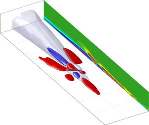
  $Q_R$) associated with BF events, whilst the remaining 29 % are associated with a varicose (symmetric) mode. Figure 3 depicts a top view of the conditional flow structures of high (red isosurface), low (grey isosurface) streamwise velocity fluctuation, and the vortex (green isosurface) associated with the existence of a negative WSS event at the wall before, during and after the BF event has been generated. The conditional averages shown in figure 3 were computed for a left-pointed vortex. Interestingly, the present conditional fields show that the asymmetric vortices identified by Guerrero et al. (Reference Guerrero, Lambert and Chin2020) are associated with an asymmetric streak interaction that exhibits similarities with the asymmetric breakdown that occurs in TBL bypass transition (Brandt & de Lange Reference Brandt and de Lange2008), which in turn is related to sinuous secondary instabilities (Brandt et al. Reference Brandt, Schlatter and Henningson2004; Schlatter et al. Reference Schlatter, Brandt, de Lange and Henningson2008).

Figure 3. Top view of the high momentum isosurface at  $\left \langle u_x\right \rangle ^+_{BF} = 0.8$ (red), low speed streak at
  $\left \langle u_x\right \rangle ^+_{BF} = -0.2$ (grey) and oblique vortex at a level
  $\left \langle Q\right \rangle ^+_{BF} = 0.5$ (green). The red and black centre lines (
 $-\cdot -$), corresponding to the orientation of the high- and low-momentum structures, respectively, depict the asymmetric interaction between these structures associated with a BF event. The three conditional fields have been computed at (a)
  $t^+ = -8.5$, (b)
  $t^+ = 0$ and (c)
  $t^+ = 8.5$.
4.2. Streak collision and breakdown process
Figure 4 exhibits a series of consecutive plots of the conditional field of streamwise velocity fluctuation  $\left \langle u_x\right \rangle _{BF}^+$ over a period
  $-43 < t^+ < 21$ associated with a left-sided (
 $Q_L$) vortex, whose circulation motion generates a negative wall-friction event at the wall. Before discussing this sequence of events, it is essential to note that two large-scale coherent structures, a forward-leaning structure of high momentum and a lifted LSS, interact to generate the BF event, as briefly shown in the previous section. The lifted LSS is sustained by the upwash motions induced by two large-scale counter-rotating streamwise rolls (Guerrero et al. Reference Guerrero, Lambert and Chin2020; Tong et al. Reference Tong, Bhatt, Tsuneyoshi and Tsuji2020), located at both sides of the streak. It should also be noted that the centroid of the high-momentum structure is located at a higher wall-normal position compared with the LSS. Hence, the high-momentum structure travels at a higher convection velocity than the LSS. Interestingly, this configuration of the conditional HSS/LSS exhibits some similarities with the flow structures obtained by analysing the first antisymmetric space–time proper orthogonal decomposition mode conditioned for extreme dissipation events in turbulent channel flow by Hack & Schmidt (Reference Hack and Schmidt2021).

Figure 4. Time dependency of the streamwise velocity fluctuations conditioned by  $Q_L$ negative WSS events. The negative values of time show the sequence of conditional events preceding the appearance of a BF event. Here
  $t^{+} = 0$ is the time at which the negative WSS appears. The positive time sequences show the evolution of the streamwise velocity structures that take place after a BF event happens. The
  $x - y$ contour plots show the conditional field
  $\left \langle u_x \right \rangle ^+_{BF}$ at
  $\Delta R \theta = 0$. The arrows indicate the flow direction. Here (a)
  $t^+ = -43$; (b)
  $t^+ = -26$; (c)
  $t^+ = -8.5$; (d)
  $t^+ =0$; (e)
  $t^+ = 15$; (f)
  $t^+ = 21$.
In figure 4(a) ( $t^+ = -43$) it is observed that the high-momentum structure approaches the LSS. As these structures approximate each other, as observed in figure 4(b), a lifted shear layer is generated at the interface of the two structures. The conditional field exhibited in figure 4(c) (
 $t^+ = -8.5$) shows that the LSS acts as a blockage to the trajectory, followed initially by the HSS moving in the streamwise direction. As a result, a depression is formed at the interface between the high- and low-momentum structures, which is simultaneously associated with the roll-up of a strong shear layer as suggested by Goudar, Breugem & Elsinga (Reference Goudar, Breugem and Elsinga2016) and Lee et al. (Reference Lee, Hutchis and Monty2019). As observed previously in figure 2, the streak collision generates an inflectional velocity profile with similar topology to the one described by Kim et al. (Reference Kim, Kline and Reynolds1971). The local inflectional velocity profile is related to a maximum attained in the vorticity field. It is also noted that as the high- and low-momentum structures collide, an azimuthal vortex located at the buffer becomes evident.
Later, figure 4(d) shows the moment when the BF at the wall emerges ( $t^+ = 0$). In that panel, it is observed that the HSS continues penetrating the LSS towards the wall, and the azimuthal vortex progressively tilts towards the streamwise direction. After the BF event has been generated (
 $t^+>0$), the oblique vortex continues stretching and reorientating mainly due to the high magnitudes of
  $\partial U_x/\partial \theta$ exiting at the left-hand side (
 $\Delta R\theta \approx 25 - 50$) of the oblique
  $Q_L$ vortex. Figure 4(e), computed at
  $t^+ \approx 15$, reveals that the tilted and stretched vortex, whose local enstrophy has been intensified, transports high-momentum towards the wall at its downwash flank. As a result, the LSS breaks down near its trailing end, and it is divided into a small- and a large-scale structure owing to the collision of the high and low-momentum structures. The dominant mechanisms by which the vortex intensifies its enstrophy are explained later in § 5.
As time progresses ( $t^+ > 15$), the small-scale structure of low-momentum, which split from the large scale LSS, is dissipated, possibly by viscous diffusion, as shown in figure 4(f). In the same figure, it is observed that both LSM, the LSS and the high momentum structure maintain their coherence and keep interacting as observed in the shear layer existing at the interface of these flow structures. By recalling the instantaneous fields observed in figures 1 and 2, after the breakdown of the LSS, often, another vortex autogenerates, usually at the trailing end of the downstream broken section of the LSS. Nevertheless, the conditional average does not show a subsequent vortex autogeneration as this process may occur in different positions in the streamwise direction, and these effects are diffused with the conditional averaging. By tracking each of the BF events analysed in this study in space and time, it was determined that 50.4 % of the negative skin friction events are followed by at least one vortex autogeneration, which subsequently produced another BF event at the vicinity of the negative WSS tracked. An analysis of the regeneration frequency and its probability is presented later in § 5.1.
From the results shown in figures 1 and 4, it is determined that the existence of a LSS is not the only condition required to induce the autogeneration of a vortex and, subsequently, a BF event. Indeed, the results show that a large-scale structure of high-momentum located upstream from the LSS is also indispensable as it produces an inflectional instability and a lifted shear layer that precede the spontaneous formation of an azimuthal vortex tube. Although the previous observations are fundamental to understanding the mechanisms by which a vortex is autogenerated, there arise several questions such as: What is the mean convection velocity of the two large-scale structures of streamwise fluctuation colliding between each other? Since vorticity is not generated within the interior of the fluid (i.e. it is generated at the flow boundaries) (Batchelor Reference Batchelor1967; Morton Reference Morton1984), it is also natural to ask which mechanisms induce a vorticity intensification in the shear layer located between the high- and low-momentum structures, so that a vortex tube appears spontaneously. If there is a series of autogenerations due to the interactions of the LSMs after a BF event is identified, it would be insightful to determine the average time between autogenerations and how many BF events can autogenerate on the same LSS.
4.3. Convection velocity of the coherent structures
The first of the questions posed above can be answered by analysing the space–time correlation of the high- and low-momentum structures, shown in figures 5(a) and 5(b), respectively. The fit of the peaks in the correlation reveals that the high-momentum structure advects at a convection velocity  $U_{c,HSS}^+ = 15.2$, whereas the LSS convects at
  $U_{c,LSS}^+ = 12.0$. It is also interesting to note that around the time at which the negative WSS event is generated, and the LSS breaks down (i.e.
  $0\leq t^+ \leq 12$), the convection velocity of the low-momentum structure drops and has a value of
  $U_{c,BF} = 9.83$, which agrees well with the mean velocity at which negative skin friction events are transported, as reported by Cardesa et al. (Reference Cardesa, Monty, Soria and Chong2014).

Figure 5. Space–time correlation of the ( $a$) high- and (
 $b$) low-momentum structures exhibited in figure 4. The
  $\times$ symbol depicts the peak of the correlation and the (dashed line) line shows the best fit of the peaks in
  $R_{u_z u_z}$. The best fit of the peaks in the correlation of the high- and low-momentum structures responds to (
 $a$)
$a$)  $\Delta x^+ = 15.2 \Delta t^+ + 0.26$ and (
 $b$)
$b$)  $\Delta x^+ = 12.0 \Delta t^+ + 22$. The line (blue dashed dotted line) in panel (b) exhibits the best fit of the peaks in the correlation at
  $0 \leq t^+ \leq 10$ and follows the linear expression
  $\Delta x^+ = 9.83 \Delta t^+$.
5. Vorticity intensification mechanism
Here we examine the vorticity dynamics associated with the spontaneous generation of the azimuthal/oblique vortex before a reverse flow event occurs.
The Helmholtz vorticity equation for an incompressible homogeneous fluid is defined as
 \begin{equation} \frac{{\rm D}{\omega_i}}{{\rm D}t} = \omega_j \frac{\partial U_i}{\partial x_j} + \nu \frac{\partial^2 \omega_i}{\partial x_j \partial x_j}. \end{equation}
 Equation (5.1) expresses that the rate of change of vorticity within the fluid ( $D \boldsymbol {\omega } / Dt$) has two main contributions. The first term on the right-hand side represents the tilting and stretching of an infinitesimal vortex line, and the second represents the viscous diffusion of vorticity (Batchelor Reference Batchelor1967). The vortex stretching term is the most important contributor to enstrophy (
 $\varOmega$) production (Landahl & Mollo-Christensen Reference Landahl and Mollo-Christensen1992). This term, which has no counterpart in the momentum equation, is responsible for maintaining the energy cascade by transferring energy from the large to the small scales of motion (Davidson Reference Davidson2004). The local vorticity stretching can be a misleading parameter to understand whether there is a vorticity intensification or not, as there are vortices with opposite signs. As a result, there exist regions with positive or negative values where a vortex is stretched or contracted. Hence, the enstrophy
  $\varOmega = \omega _i\omega _i/2$ equation provides a more robust way to identify the regions where vorticity is intensified due to stretching. The enstrophy equation can be derived from (5.1), and it responds to the following expression:
 \begin{equation} \frac{{\rm D}}{{\rm D}t} \left(\frac{\varOmega}{2}\right) = \omega_i \omega_j \frac{\partial U_i}{\partial x_j} + \nu\nabla^2 \left( \frac{\varOmega}{2}\right) - \nu\frac{\partial \omega_i}{\partial x_j} \frac{\partial \omega_i}{\partial x_j}. \end{equation}
The first term on the right-hand side of (5.2) corresponds to the amplification or reduction of enstrophy due to the stretching/tilting or compression of vortex lines. The two last terms on the right-hand side express the diffusion and dissipation of enstrophy, respectively. Here we are interested in analysing the mechanics associated with enstrophy production (note that the terms enstrophy production/intensification due to stretching will be used interchangeably hereinafter). Hence, we shall focus on the conditionally averaged nonlinear enstrophy production by stretching, which couples vorticity and strain as
 \begin{equation} \left\langle\omega_i \omega_j\frac{\partial U_i}{\partial x_j}\right\rangle^+_{BF}. \end{equation}
 The norm of the direct stretching terms from (5.3) in the three orthogonal directions has been computed as a function of time over a wall-parallel plane located at  $y^{+}\approx 12$ to determine the dominant mechanism by which enstrophy is amplified. This position was selected because the buffer vortex's core that generates the BF event is at this location. The outcome of this calculation is depicted in figure 6(a). The results reveal that between
  $-20 \lesssim t^{+} \lesssim 1$, the enstrophy is intensified in the three directions. The same figure also reveals that the azimuthal (black) and the streamwise (blue) components experience a substantial growth. Nevertheless, the
  $\theta$-component seems to be the dominant mechanism of enstrophy production as it exhibits the highest magnitude and is intensified at a higher rate at
  $t^+ > -10$. It is noted that the azimuthal term of enstrophy production attains a maximum at
  $t^{+}\approx 1$. This is coincident with the instant at which the reverse flow event at the wall attains a minimum (see figure 6b).

Figure 6. (a) Time dependence of the enstrophy intensification norm in the three orthogonal directions computed over a wall-parallel plane at  $y^{+}\approx 12$. The colours represent the radial component (red), azimuthal component (black) and the streamwise component (blue). The norm has been computed on each of the time-dependent conditional fields as
  $\max \{\omega _i \omega _j \, \partial U_i/\partial U_j({\boldsymbol x},t) \}_{BF}$. (b) Time evolution of the minimum WSS in the streamwise direction
  $\left \langle \tau _{w,x} \right \rangle _{BF}^+$ within the conditional flow fields.
The three direct stretching terms (i.e.  $\omega _i \omega _i\,\partial U_i / \partial _{x_i}$), which contribute to each of the orthogonal components of (5.3), have been similarly analysed. It was observed that the major contribution to the enstrophy amplification comes from the
  $\theta$-direct stretching
  $\left \langle \omega _\theta ^2/r ~(\partial U_\theta / \partial \theta ) \right \rangle _{BF}^{+}$. It is noteworthy that the temporal evolution of the minimum in the WSS (figure 6b) exhibits a mirror-like behaviour about the norm of the enstrophy intensification on the
  $\theta$-direction. Indeed, as mentioned previously, the minimum attained by the function min(
 $\tau _w$) coincides with the maximum reached by the azimuthal component of enstrophy intensification. Hence, these results show that reverse flow events correlate with a region with high
  $\theta$-enstrophy production occurring at the buffer region. In other words, these findings suggest, from a statistical perspective, that BF events are associated with the autogeneration of an azimuthal or oblique vortex.
The results shown in figure 6 have revealed that the enstrophy (or vorticity) intensification in the azimuthal direction by direct stretching seems to be the dominant mechanism by which the vortex responsible for a reverse flow at the wall is autogenerated, from a statistical standpoint. However, to better understand the three-dimensional flow dynamics associated with this mechanism, the  $\left \langle \omega _\theta ^2/r ~\partial U_\theta / \partial \theta \right \rangle _{BF}^{+}$ has been computed for the series of conditional fields associated with the generation of a BF event. The sequential plots depicted in figure 7 exhibit the time evolution of the regions of azimuthal enstrophy intensification due to stretching (red isosurface) and dampening due to contraction (blue isosurface). The
  $x - y$ contour plots presented in figure 7(a–d) have been computed at
  $\Delta R\theta = 0$. These contour plots show that, for the events analysed in this study, a layer of positive azimuthal vorticity is lifted and intensified (red contour) due to the collision between the high- and low-momentum structures explained previously. The negative values of azimuthal intensification (blue contour) show that vorticity is reduced by the contraction of vortex lines within the LSS.

Figure 7. Time dependence of the conditional enstrophy amplification in the azimuthal direction  $\left \langle \omega _\theta ^2/r \, \partial U_\theta / \partial \theta \right \rangle _{BF}^{+}$ due to vortex line stretching. The grey isosurface is the LSS. The enstrophy intensification has been normalised in wall units by
  $(u_\tau ^2/\nu )^3$. The red (positive) and blue (negative) isosurfaces have been computed at a level
  $\left \langle \omega _\theta ^2/r\, \partial U_\theta /\partial \theta \right \rangle ^+_{BF} = \pm 4.5\times 10^{-4}$, respectively. The colour contours exhibited in the
  $x - y$ plane correspond to the enstrophy intensification in the azimuthal direction. The vector plots exhibited in the
  $R \theta - y$ planes
  $b_1$ and
  $b_2$ have been computed at
  $t^+ = -8.5$ at locations
  $\Delta x^+ = -50$ and
  $\Delta x^+ = -250$, respectively. The red contours in planes
  $b_1$ and
  $b_2$ highlight the regions with high positive
  $\theta$ enstrophy intensification by direct stretching, and the blue line contours correspond to the LSS. The orange and blue transparent arrows exhibited on the transverse sections
  $b_1$ and
  $b_2$ aim to highlight the outer and the inner streamwise rolls that sustain the high- and the low-momentum structures associated with a BF event, respectively. Here (a)
  $t^+ = -26$; (b)
  $t^+ = -8.5$; (c)
  $t^+ = 0$; (d)
  $t^+ =15$.
Although the collision between high/low-momentum structures is a plausible mechanism to lift shear, it does not fully explain how the vorticity sheet, existing at the trailing end of the LSS, is stretched in the azimuthal direction. A series of transverse vector plots provide a simple way of examining the azimuthal stretching ( $1/r~\partial U_\theta / \partial \theta$). The
  $R\theta - y$ vector plots exhibited in figure 7(b) show that upstream from the LSS (plane
  $b_2$), the high momentum structure that collides with the LSS is associated, on average, with the downwash motions induced by a pair of outer streamwise rolls, whose cores seem to be located at the overlap region. These rotating motions contribute to the sustenance of the HSS by transporting momentum towards the wall and generating a large-scale structure of strong sweep. In the same vector plot (plane
  $b_2$), within the viscous sublayer, at
  $-25\leq \Delta R\theta ^+ \leq 25$ it is observed that
  $U_\theta$ diverges. Consequently, the large local values of azimuthal stretching intensify the vorticity sheet below the large structure of high momentum.
Downstream, the vectors of plane  $b_1$, computed at
  $\Delta x^+ =-50$, show that the LSS is lifted at the upwash flank of two inner counter-rotating rolls located at the buffer region. In this position, the high momentum structure is located above the LSS (refer back to figure 4c), and it is associated with the downwash side of the outer counter-rotating rolls, highlighted with orange arrows in plane
  $b_1$. In that figure, the velocity vectors show that at
  $y^+ \approx 30$ and
  $-25 \leq \Delta R \theta ^+ \leq 25$, there exists a saddle node. This saddle node is caused by the counter-rotating motions mentioned above and highlighted in plane
  $b_1$. Consequently, the azimuthal velocity component diverges at this location, stretching the local high streamwise vorticity situated at the interface of the high- and low-momentum structures that collide. As a result, a significant enstrophy intensification of the aforementioned vorticity sheet at the buffer region is produced. This structure with high values of enstrophy brings to life the identifiable azimuthal vortex observed previously in figure 4(c). Simultaneously, this vortex, generated by the enstrophy intensification of a vortex sheet, is responsible for giving to the LSS the characteristic depression in its trailing end observed in BF events (Chin et al. Reference Chin, Vinuesa, Örlü, Cardesa, Noorani, Chong and Schlatter2020) and critical points (Cardesa et al. Reference Cardesa, Monty, Soria and Chong2014; Chin et al. Reference Chin, Monty, Chong and Marusic2018). As time progresses, this region, where
  $U_\theta$ diverges, continues stretching the vortex lines and intensifying the vortex's local enstrophy. Subsequently, a BF appears, and this vortex tilts towards the
  $x$-direction and contributes to the streak breakdown, as explained previously in § 4. This series of events shows that as two large-scale structures interact, energy is transferred to increase a vortex's angular velocity by stretching vortex lines.
As previously observed in figure 6(a), the streamwise component of enstrophy amplification provides the other relevant contribution to enstrophy production. As a result, the direct stretching term of enstrophy amplification in the streamwise direction has been computed and is exhibited in figure 8 at three different stages. First, it should be noted that the sequence shown in figure 8 is shorter than the one presented for the azimuthal term (figure 7) as the activity in the  $x$ stretching term is perceptible recently at
  $t^{+} \approx -10$. Similarly, in figure 8(a–c), the grey isosurface represents the LSS, and the red and blue isosurfaces are regions of positive and negative streamwise enstrophy intensification by direct stretching in the
  $x$-direction. The red isosurface, related to streamwise intensification, shows an interesting sequence of events. First, at
  $t^{+}=-8.5$, which is the exact moment at which the azimuthal vortex becomes noticeable, a small-scale region of
  $\omega _x$ amplification by stretching is observable within the buffer region at the left flank of the LSS (figure 8). Later, at
  $t^{+}=0$, when the BF occurs, the structure of streamwise intensification has stretched, and its shape exhibits a similar topology, orientation and length as the oblique vortex that generates a reverse flow at the wall. As time progresses, the positive
  $\omega _x^2\,\partial U_x/\partial x$ structure continues tilting and aligns towards the
  $x$-direction, exhibiting a topology of a quasi-streamwise vortex.

Figure 8. Time dependence of the conditional enstrophy amplification in the streamwise direction  $\left \langle \omega _x^2 ~\partial U_x / \partial x \right \rangle _{BF}^{+}$ due to direct stretching. The grey isosurface is the LSS. The enstrophy intensification has been normalised in wall units by
  $(u_\tau ^2/\nu )^3$. The red (positive) and blue (negative) isosurfaces have been computed at a level
  $\left \langle \omega _x^2 ~\partial U_x / \partial x \right \rangle _{BF}^{+} = \pm 4.0\times 10^{-5}$, respectively. Here (a)
  $t^+ = -8.5$; (b)
  $t^+ = 0$; (c)
  $t^+ = 8.5$.
In summary, from a vorticity dynamics perspective, the present results show that the precursors of a BF event are the collision of structures travelling at different convection velocities. As the collision occurs, a shear layer with high local values of  $\omega _\theta$ at the interface of the high- and the low-momentum structures arises. Simultaneously, the counter-rotating motions that sustain these high and low streamwise fluctuation structures generate a saddle node in the
  $\theta - y$ plane. Consequently, local high values of
  $\partial U_\theta / \partial \theta$ are produced in this region, and it induces the intensification of enstrophy by stretching. Subsequently, an azimuthal or oblique vortex tube arises in this region owing to the
  $\theta$ intensification. The present findings have clearly illustrated the nonlinear mechanism associated with the generation of extreme events and small dissipative scales. In the context of this investigation, we have unveiled that streak collision, followed by a shear layer formation, which later experiences direct stretching in the azimuthal direction, are the dominant mechanisms by which azimuthal/oblique vortices, BF events, and the streak breakdown are produced.
5.1. Autogeneration time
After examining the series of vortex and negative WSS autogenerations, the question naturally arises of how often BF autogenerations are observed after a negative WSS event has been localised. Also, it is natural to think about how many negative  $\tau _w$ events can be generated after a nascent BF is tracked in space and time. Consequently, the probability distribution of the regeneration time between BF events and the number of times that BFs autogenerate within the same LSS have been computed. It should be mentioned that to analyse whether a BF autogenerates after a previously identified reverse flow event, the following algorithm has been implemented.
(i) A nascent BF event is identified by performing the two-dimensional correlation between the BF patches of two consecutive flow fields.
(ii) As a new negative WSS patch has been identified, it is tracked in time following a method similar to Lozano-Durán & Jiménez (Reference Lozano-Durán and Jiménez2014) during a period of 30 ‘+’ temporal units (
 $\Delta t^+ = \Delta t u_\tau ^2 / \nu$). The sampling box used to track the BF patch in time has a size $-30 \leq \Delta x^+ \leq 420$ and $-40 \leq \Delta R\theta \leq 40$ in the streamwise and azimuthal directions, respectively. Also, the centroid of the original BF event is located at the coordinates $(0,0)$ of the sampling grid.
(iii) To ensure that the BFs are regenerated below the same LSS, the regeneration and the original BF need to happen over a continuous region where
$\tau _w^+<1$. Otherwise, the regeneration is not accounted for as it would be related to a different structure. (Note that a region of $\tau _w^+ < 1$ at the wall could be understood as the footprint of a LSS (Hutchins et al. Reference Hutchins, Monty, Ganapathisubramani, Ng and Marusic2011).)(iv) If a BF patch splits or merges, it is not considered as an autogeneration.
(v) The autogeneration time between BF patches is considered as the difference between the time a nascent BF event is identified and the time a new negative WSS event appears.


Figure 9(a) shows the probability distribution of the regeneration time  $\Delta t^+$ between BF events that occur on the same LSS. The probability distribution presented here only accounts for the BF events autogenerated at least once after a new BF event is identified. From the current data set, it was observed that approximately 50 % of the BF events tracked regenerated at least once. Figure 9(a) also shows that the mean autogeneration time of a BF event occurring after a negative WSS has been identified is
  $\Delta t^+ \approx 11$. Also, the probability distribution of the BF events suggests that they most likely regenerate after
  $\Delta t^+ \approx 3 - 5$ as the probability distribution peaks at
  $\Delta t^+ \approx 4.5$. Due to the time resolution used in this study
  $(\Delta t^+ \approx 1)$, it is not possible to capture the BF events that regenerate over smaller time scales.

Figure 9. (a) Probability density function (p.d.f.) of the regeneration time of negative WSS events. (b) Probability distribution of the number of BF autogenerations.
The probability distribution of the number of subsequent regeneration cycles experienced by a BF event is exhibited in figure 9(b). The intersection of the p.d.f. with the ordinate shows that approximately 50 % of the BF events tracked in this study do not regenerate. On the other hand, the other 50 % of BF events tracked in time are followed by other BF autogenerations that occur later over the same LSS. The maximum number of BF autogenerations found using the algorithm described previously is seven. Such a large number of autogenerations following a nascent BF event (seven regenerations) was found only once in 3266 BF events analysed, which implies 0.03 % of probability of occurrence. This suggests that observing more than seven regenerations occurring after a BF event would be an improbable phenomenon, considering that negative wall-friction patches at the wall are already rare events.
6. Concluding remarks
6.1. Precursors of BF events
The present investigation aims to understand the precursors of rare BF events at the wall. To achieve that, we have analysed volumetric DNS time series of turbulent pipe flow at  $Re_\tau \approx 1000$ with a high spatiotemporal resolution. By tracking the flow structures associated with BF events in instantaneous and conditionally averaged flow fields, it is observed that BF events result from the collision of two large-scale structures travelling at different convection velocities. The two essential flow structures are a LSS located at the near-wall region with a streamwise length
  $\Delta x^+ \approx 3R$ and a forward inclined HSS located upstream from the LSS.
The space–time correlations of the high- and the low-momentum structures revealed that, on average, these structures travel at convection velocities  $U_{c,HSS}^+ = 15.2$ and
  $U_{c,LSS}^+=12.0$. Consequently, the high-momentum structure approaches and collides with the LSS. It should be mentioned that the present results suggest that this collision is usually asymmetric and is associated with the sinuous patterns followed by the LSSs. As a result of the collision, a local unstable inflectional profile is generated. This instability, in turn, is related to the lifting of a layer with a high magnitude of vorticity located at the interface of the HSS and the LSS, specifically at the buffer region and at the trailing end of the LSS. As time progresses, an identifiable spanwise or oblique vortex arises at the location where the lifted shear layer exists. As this vortex increases its local enstrophy by stretching and tilting, its circulation motion generates a BF event. Approximately
  $12+$ temporal units after the BF arises, the vortex induces the breakdown of the LSS by transporting high momentum from the HSS structure towards the wall. As a result, the LSS splits into a large-scale section and a small-scale part.
6.2. Nonlinear mechanism of vortex autogeneration
The structure collision clearly shows the formation of a lifted shear layer at the interface of the HSS and the LSS, which has high values of azimuthal vorticity. However, the streak collision by itself is inadequate to explain how vortex lines are intensified to generate an azimuthal vortex tube spontaneously. As a result, the nonlinear coupling between enstrophy and strain from the enstrophy equation, also known as enstrophy production/intensification by stretching, has been analysed. The results from the time-dependent norm of these quantities and conditionally averaged fields indicate that the dominant mechanism is the direct stretching in the azimuthal direction  $\left \langle \omega _\theta ^2/r ~(\partial U_\theta / \partial \theta ) \right \rangle _{BF}^{+}$, as this term is significantly higher than the other stretching terms in the three orthogonal directions. The region where
  $\omega _\theta$ is intensified by stretching is located at the same position at which the azimuthal or oblique vortex associated with a BF event appears. The azimuthal stretching
  $(1/r~ \partial U_\theta / \partial \theta )$ amplifies the enstrophy of the shear layer, and the subsequent azimuthal vortex tube is generated within a region where the azimuthal velocity diverges at the buffer region. This high azimuthal stretching is associated with a saddle node induced by the counter-rotating streamwise rolls attached to the wall that sustain the LSS and the outer counter-rotating rolls, which transport high momentum towards the wall and sustain the HSS. After the azimuthal/oblique vortex appears, its leading end is stretched in the streamwise direction as it is transported with the high momentum structure surrounding the LSS. As time progresses, the vortex continues stretching and reorientates in the streamwise direction and becomes a quasi-streamwise vortex. Hence, the present results provide a plausible explanation of the nonlinear mechanism and the associated flow structures by which a buffer vortex can be autogenerated and how it evolves and turns into a streamwise vortex.
The findings reported in this investigation resulted from examining the temporal evolution of the flow structures associated with rare BF events at the wall. Although BF patches could be understood as rare events that barely contribute to the total mean shear stress, the present results suggest that reverse flow events are associated with fundamental and essential mechanisms in turbulent flows. Indeed, our results imply that a BF event can be viewed as the signature of an azimuthal/oblique vortex that has been autogenerated by nonlinear mechanisms, specifically stretching. Moreover, the results reported in this investigation show consistency with previous studies regarding the SSP of near-wall turbulence (Jiménez & Moin Reference Jiménez and Moin1991; Hamilton et al. Reference Hamilton, Kim and Waleffe1995; Schoppa & Hussain Reference Schoppa and Hussain1997; Heist & Hanratty Reference Heist and Hanratty2000; Schoppa & Hussain Reference Schoppa and Hussain2002; Bae et al. Reference Bae, Lozano-Durán and McKeon2021). Most of these previous studies have been conducted in reduced-order systems. It should be mentioned that the autogeneration mechanism described in this paper is not the only plausible mechanism of vortex regeneration.
Besides detailing the precursors and consequences of a vortex regeneration and a BF event, this investigation provides a suitable method for tracking the nonlinear mechanism of vortex regeneration. Although it is well known that a LSS plays an essential role in the SSP, tracking the clusters of reverse flow events provides an accurate location of the nonlinear autogenerations happening within an unconstrained flow. As a result, this opens the door to other researchers who could use, in this context, more sophisticated analysis tools and provide further insight into the nonlinear mechanisms of the near-wall SSP.
As a final remark, it is worth mentioning that the present knowledge can be adapted to flow control techniques. From our understanding, some of the current approaches aim to detect HSS, which triggers an active flow control actuator to disrupt the flow. Active flow control techniques have been proved to be effective repeatedly. Nevertheless, our results suggest that a possible improvement to the current flow control techniques would be applying active control methods not only in the regions where a HSS is localised but also where a possible streak collision will happen (i.e. when a LSS is detected followed by a high-momentum structure).
Funding
This work was supported with supercomputing resources provided by the Phoenix HPC service at the University of Adelaide. This research was also undertaken with the assistance of resources provided at the NCI NF through the Computational Merit Allocation Scheme, supported by the Australian Government and the Pawsey Supercomputing Centre, with funding from the Australian Government and the Government of Western Australia. The authors acknowledge the financial support of the Australian Research Council.
Declaration of interests
The authors report no conflict of interest.


