


1. Introduction
The presence of coherent long-lived vortices is a ubiquitous and fascinating feature of most turbulent geophysical flows (e.g. Carton Reference Carton2001; Sokolovskiy & Verron Reference Sokolovskiy and Verron2014). Our focus is on the dynamics of oceanic vortices, exemplified by the Gulf Stream and Agulhas rings, which can persist for years and sustain hundreds of revolutions. Such vortices can propagate thousands of kilometres away from their points of origin (Robinson Reference Robinson1983; Olson Reference Olson1991), transporting water masses with distinct physical and chemical properties trapped in their cores across the ocean basins. The associated lateral eddy-driven mixing affects large-scale circulation patterns, the ocean climate and the dispersion of pollutants (Masumoto et al. Reference Masumoto2012; Dong et al. Reference Dong, McWilliams, Liu and Chen2014; Pérez-Hernández et al. Reference Pérez-Hernández, McCarthy, Vélez-Belchí, Smeed, Fraile-Nuez and Hernández-Guerra2015). Coherent vortices also have a tangible impact on regional and global ecosystems (e.g. McGillicuddy Reference McGillicuddy2016), motivating efforts to fully understand their dynamics and transport characteristics.
The advent of satellite-based methods of analysis and high-resolution global simulations offer previously inaccessible statistical descriptions of the propagation tendencies of coherent eddies (Chelton, Schlax & Samelson Reference Chelton, Schlax and Samelson2011; Petersen et al. Reference Petersen, Williams, Maltrud, Hecht and Hamann2013; Samelson, Schlax & Chelton Reference Samelson, Schlax and Chelton2014; Chen & Han Reference Chen and Han2019). Both observations and comprehensive simulations consistently indicate that, on average, coherent vortices migrate westward (e.g. Chassignet, Olson & Boudra Reference Chassignet, Olson and Boudra1990; Olson Reference Olson1991; Chelton, Schlax & Samelson Reference Chelton, Schlax and Samelson2011). This tendency is commonly attributed to the variation of the planetary vorticity with latitude, known as the beta-effect. The connection between the westward drift of geophysical vortices and the beta-effect was first established in the pioneering studies of Rossby (Reference Rossby1948) and Adem (Reference Adem1956). Numerous subsequent investigations – theoretical, numerical and experimental – confirmed this link and further elucidated the physical mechanisms at play (e.g. Reznik & Dewar Reference Reznik and Dewar1994; Sutyrin & Flierl Reference Sutyrin and Flierl1994; Sutyrin et al. Reference Sutyrin, Hesthaven, Lynov and Rasmussen1994; Llewellyn Smith Reference Llewellyn Smith1997; Flór & Eames Reference Flór and Eames2002). In particular, a series of analytical models have been developed (McWilliams & Flierl Reference McWilliams and Flierl1979; Nof Reference Nof1981, Reference Nof1983; Killworth Reference Killworth1986; Cushman-Roisin, Chassignet & Tang Reference Cushman-Roisin, Chassignet and Tang1990; Benilov Reference Benilov1996) which express the migration rate of isolated vortices in terms of eddy structure and background stratification. While based on differing assumptions and approaches, these theories consistently suggest that the preferred motion pattern is westward, and the magnitude of propagation velocity is comparable to the speed of long Rossby waves
 \begin{equation}U\sim{-} \beta R_d^2,\end{equation}
where  $\beta = \partial f/\partial y$ is the meridional gradient of the Coriolis parameter (f) and
  ${R_d}$ is the first baroclinic radius of deformation. Although the fluid-dynamical significance of the migration-rate theories is hard to overestimate, attempts to validate them by observations and comprehensive numerical models have not been uniformly satisfying. For instance, propagation velocities (1.1) in most ocean regions are of the order of
  $U\sim 1\;\textrm{cm}\;{\textrm{s}^{ - 1}}$. However, vortices often drift faster, by as much as an order of magnitude, and their trajectories can be significantly non-zonal (e.g. Cornillon, Weyer & Flierl Reference Cornillon, Weyer and Flierl1989; Chassignet, Olson & Boudra Reference Chassignet, Olson and Boudra1990; Byrne, Gordon & Haxby Reference Byrne, Gordon and Haxby1995; Nof et al. Reference Nof, Jia, Chassignet and Bozec2011). The recent analysis of altimeter data reveals that random movement in various directions is a ubiquitous feature of eddies throughout the world ocean (Ni et al. Reference Ni, Zhai, Wang and Marshall2020). The discrepancies between the observed movement of eddies and their nominal beta-induced drift speeds are commonly attributed to the advection by the background flow (e.g. Chen & Han Reference Chen and Han2019), the action of the wind stress (e.g. Nof et al. Reference Nof, Jia, Chassignet and Bozec2011) and the interaction between eddies (e.g. Early, Samelson & Chelton Reference Early, Samelson and Chelton2011; Ni et al. Reference Ni, Zhai, Wang and Marshall2020).
Our study examines yet another potential cause of variability in eddy migration rates, which has previously been analysed only to a limited extent (Radko & Stern Reference Radko and Stern1999; Voropayev et al. Reference Voropayev, McEachern, Boyer and Fernando1999). We shall focus on the self-propagation of vortices due to the presence of a weak dipolar component, which could often be masked by the dominant axisymmetric circulation (e.g. Stern Reference Stern1987; Radko Reference Radko2020). One of the causes of non-axisymmetric flow patterns in geophysical vortices is the beta-effect, which can naturally generate the dipolar component by modifying an initially axisymmetric vortex (Adem Reference Adem1956). This dipolar component – often referred to as the beta gyre – induces vortex motion that is initially non-zonal. However, the interaction between the beta gyres and axisymmetric component eventually results in the predominantly westward drift of the vortex with a velocity comparable to the speed of long Rossby waves (e.g. Sutyrin & Flierl Reference Sutyrin and Flierl1994). The radiation of Rossby waves by moving vortex can produce some residual meridional motion and the reduction in its zonal speed (e.g. Nycander Reference Nycander2001; Kravtsov & Reznik Reference Kravtsov and Reznik2019). However, for strong eddies, such as considered here, these effects are generally mild.
For the present discussion, it should be emphasized that the beta-effect is not the only source of dipolar components in geophysical eddies. The dipolar pattern can be produced through the vortex interactions with topography, coastlines, wind forcing or ambient flow patterns (e.g. Stern & Radko Reference Stern and Radko1998; Radko Reference Radko2008). It can also be created by the same process that generated the vortex in the first place. Once introduced, the dipolar component of non-beta origin can persist for lengthy periods, controlling the vortex dynamics and trajectory. A distinct line of conceptual models reflecting the role of dipolar components in the vortex dynamics is based on the exact ‘modon-with-the-rider’ solutions (Flierl et al. Reference Flierl, Larichev, McWilliams and Reznik1980). The term modon, coined by Stern (Reference Stern1975) as a neat reference to then ongoing observational MODE program (Pedlosky Reference Pedlosky2010), represents the dipolar part of a vortex, and ‘rider’, its axisymmetric component. Solutions of this type propagate zonally, and their velocities can attain a wide range of values that are determined by the strength of the dipolar component. However, there is a principal complication that limits the use of modon-with-the-riders as models of persistent geophysical vortices, which is their instability. Numerical simulations (Swenson Reference Swenson1987) indicate that, in the oceanographically relevant regime, where the amplitude of a circular rider exceeds the dipolar component, the entire structure rapidly disintegrates. This undesirable feature motivates the search for alternative – more stable and robust – solutions, some of which are developed in this study.
The present investigation explores the influence of initial conditions on the evolution of vortices in a series of simulations utilizing the equivalent-barotropic beta-plane model. Using the optimization algorithm described in § 2, we introduce dipolar perturbations that force vortices to translate initially with given velocity and examine their trajectories (§ 3). Simulations reveal that the motion pattern of eddies is controlled for long periods by the magnitude and orientation of their initial dipolar moments. This property is illustrated using two distinct classes of solutions, with finite (§ 3.1) and zero (§ 3.2) net angular momentum. The zero angular momentum vortex satisfies the integral condition
 \begin{equation}\iint {(\psi - {\psi _\infty })\,\textrm{d}x\,\textrm{d}y} = 0,\end{equation}
where  $\psi$ is the streamfunction, which is related to the horizontal velocity components
  $(u,v) = ( - \partial \psi /\partial y,\partial \psi /\partial x)$, and
  ${\psi _\infty }$ represents its value in the vortex far field. These solutions are characterized by the heightened sensitivity to the initial conditions relative to their finite angular momentum counterparts. In § 4, we contrast the self-propagation tendencies, and the associated physical mechanisms, of the beta-plane and f-plane vortices. To identify the essential dynamics of self-propagation, we also consider the reduced-dynamics model (§ 5). This model assumes that the magnitudes of the dipolar component and beta-effect are relatively low, and the governing equations can be linearized about the dominant axisymmetric pattern. The resulting solutions exhibit much weaker self-propagation tendencies than their nonlinear counterparts. This finding implies that the maintenance of the initial dipolar moment is greatly enhanced by fundamentally nonlinear processes. We summarize results and draw conclusions in § 6.
2. Formulation
This study is based on the equivalent-barotropic model (e.g. Pedlosky Reference Pedlosky1987)
 \begin{equation}\frac{\partial }{{\partial t}}\left( {{\nabla^2}\psi - \frac{\psi }{{R_d^2}}} \right) + J(\psi ,{\nabla ^2}\psi ) + \beta \frac{{\partial \psi }}{{\partial x}} = \nu {\nabla ^4}\psi ,\end{equation}
where J is the Jacobian and  $\nu $ represents the lateral eddy viscosity. We use (2.1) to investigate the dynamics of isolated vortices, characterized by the relatively rapid decrease of circulation in the far field:
  $|\psi |\le O({r^{ - 2}})$, where we assume
  ${\psi _\infty } = 0$ without loss of generality. One of the earliest and most fundamental results in the vortex theory is the estimate of beta-induced migration rates based on the centroid theorem (McWilliams & Flierl Reference McWilliams and Flierl1979). Because of its significance for the present investigation, this theorem is briefly reviewed below.
2.1. Centroid theorem
The explicit expression for the propagation of the centre of mass anomaly is obtained by multiplying (2.1) by  $(x,y)$ and integrating the result over the entire horizontal plane
 \begin{equation}\frac{{\textrm{d}{\kern 1pt} {x_c}}}{{\textrm{d}t}} ={-} \beta R_d^2,\quad \frac{{\textrm{d}{\kern 1pt} {y_c}}}{{\textrm{d}t}} = 0,\end{equation}
where  $({x_c},{y_c})$ are the coordinates of the eddy centroid, defined as
 \begin{equation}{x_c} = \frac{{\displaystyle\iint {x\psi \,\textrm{d}x\,\textrm{d}y} }}{{\displaystyle\iint {\psi \,\textrm{d}x\,\textrm{d}y} }},\quad {y_c} = \frac{{\displaystyle\iint {y\psi \,\textrm{d}x\,\textrm{d}y} }}{{\displaystyle\iint {\psi \,\textrm{d}x\,\textrm{d}y} }}.\end{equation}
What makes the centroid theorem even more general and surprisingly robust, is that the centre-of-mass speed of coherent vortices embedded in steady large-scale flows is still given by (2.2). This ‘anti-Doppler’ effect (Nycander Reference Nycander1994) is caused by the variation in the upper layer thickness associated with the large-scale geostrophic current. The action of the resulting environmental potential vorticity gradient is similar to the beta-effect, causing the eddy to move at the same speed but in the direction opposite to the ambient current, thereby cancelling the advective tendency of the large-scale flow. It should be realized that the exact cancellation of these tendencies occurs only in the equivalent-barotropic model and uniform large-scale currents. The anti-Doppler effect takes on a less rigid and clear-cut form in more complicated models (Nycander Reference Nycander1994) and spatially non-uniform flows (Sutyrin & Carton Reference Sutyrin and Carton2006). Nevertheless, the fact that the advection by large-scale flows has a limited effect on the vortex speed makes it imperative to explain the wide range of eddy migration rates in the ocean (Cornillon et al. Reference Cornillon, Weyer and Flierl1989; Nof et al. Reference Nof, Jia, Chassignet and Bozec2011; Ni et al. Reference Ni, Zhai, Wang and Marshall2020). We should also mention that the analogous constraints on the propagation speed of coherent vortices do not arise in the purely barotropic model. In fact, the singular character of the barotropic model made it possible to develop several analytical solutions representing self-propagating vortices and demonstrate their ability to translate over large distances on the barotropic f-plane (e.g. Stern & Radko Reference Stern and Radko1998; Radko Reference Radko2008). The explicit constraint (2.2) on the centroid speed is ultimately caused by the effects of stretching/squeezing of water columns during the vortex motion, represented by the term  $\psi /R_d^2$ in the potential vorticity (2.1).
Of course, it is possible that the velocity of the centroid simply differs from other – more local and precise – measures of the vortex movement, such as the displacement of potential vorticity extrema. The analysis of this difference is one of the key objectives of the present investigation. However, the corollary of the centroid theorem is that exact uniformly propagating solutions in the equivalent-barotropic model are possible only for the migration rate  $(U,V) = ( - \beta R_d^2,0)$. An important exception, allowing vortices to move with a wide range of speeds, is the zero angular momentum configuration (1.2). In this case, (2.2) and (2.3) are inapplicable. However, the straightforward modification of the centroid theorem leads to
 \begin{equation}\frac{\textrm{d}}{{\textrm{d}t}}\,\iint {x\psi \,\textrm{d}x\,\textrm{d}y} = 0,\quad \frac{\textrm{d}}{{\textrm{d}t}}\,\iint {y\psi \,\textrm{d}x\,\textrm{d}y} = 0,\end{equation}
which is readily interpreted as a conservation principle for the first moment of the streamfunction. Equations (2.4) also imply that if a zero angular momentum vortex contains a substantial dipolar component initially, it will be maintained indefinitely. A well-known example of zero angular momentum vortices is the family of exact modon-with-the-rider solutions (e.g. Flierl et al. Reference Flierl, Larichev, McWilliams and Reznik1980). Free from the rigid constraints of the centroid theorem, such solutions can be found for any values of zonal propagation velocities outside of the Rossby wave range  $( - \beta R_d^2 \lt {U_{Rossby}} \lt 0)$.
For both finite and zero angular momentum vortices, the question arises regarding the impact of the dipolar component on their movement and long-term evolution. This question is addressed by superimposing relatively weak dipoles on stable circularly symmetric riders and examining the evolution of the resulting systems numerically. The dipolar components producing the initial motion with a given velocity  $(U,V)$ are computed using the following optimization procedure.
2.2. Optimal non-axisymmetric perturbations
To reduce the number of controlling parameters, we non-dimensionalize (2.1) using  ${R_d}$ as the unit of length,
  $\beta R_d^2$ as the unit of velocity and
  ${(\beta {R_d})^{ - 1}}$ as the unit of time. As a result, (2.1) reduces to
 \begin{equation}\frac{\partial }{{\partial t}}({\nabla ^2}\psi - \psi ) + J(\psi ,{\nabla ^2}\psi ) + \frac{{\partial \psi }}{{\partial x}} = {\nu _{nd}}{\nabla ^4}\psi ,\end{equation}
where  ${\nu _{nd}} = \nu /(\beta R_d^3)$. Introducing the fluid potential vorticity (PV)
 \begin{equation}q = {\nabla ^2}\psi - \psi ,\end{equation}
further reduces (2.5) to
 \begin{equation}\frac{{\partial q}}{{\partial t}} + J(\psi ,q) + \frac{{\partial \psi }}{{\partial x}} = {\nu _{nd}}{\nabla ^4}\psi .\end{equation}
Since the existence of exact stable solutions of (2.5) representing quasi-monopolar vortices uniformly propagating in space is not guaranteed, we now attempt to construct some accurate approximations. For that, we consider a circularly symmetric and preferably stable rider with the PV distribution  ${q_0} = {q_0}(r)$, where
  $r = \sqrt {{x^2} + {y^2}} $, and search for a non-axisymmetric perturbation
  $q^{\prime}$ that would cause the vortex to move with a given speed
  $(U,V)$. The entire PV field is expressed in terms of its azimuthal Fourier components as follows:
 \begin{equation}q = {q_0}(r) + \sum\limits_{i = 1}^{{n_\theta }} {[{q_{ci}}(r)\,\textrm{cos}(i\theta ) + {q_{si}}(r)\,\textrm{sin}(i\theta )]} ,\end{equation}
where  ${n_\theta }$ is the number of azimuthal harmonics and
  $\theta $ is the polar angle defined by
 \begin{equation}\textrm{cos}\,\theta = \frac{x}{r},\quad \textrm{sin}\,\theta = \frac{y}{r}.\end{equation}
To find uniformly translating patterns, we rewrite the governing equation (2.7) in the coordinate system moving with the target velocity  $(U,V)$
 \begin{equation}\frac{{\partial q}}{{\partial t^{\prime}}} - U\frac{{\partial q}}{{\partial x^{\prime}}} - V\frac{{\partial q}}{{\partial y^{\prime}}} + J(\psi ,\,q) + \frac{{\partial \psi }}{{\partial x^{\prime}}} = {\nu _{nd}}{\nabla ^4}\psi ,\end{equation}
where the new independent variables  $(t^{\prime},x^{\prime},y^{\prime})$ are related to the original ones through
 \begin{equation}t^{\prime} = t,\quad x^{\prime} = x - Ut,\quad y^{\prime} = y - Vt.\end{equation}
Equation (2.10) can also be expressed in terms of the streamfunction tendency
 \begin{equation}\frac{{\partial \psi }}{{\partial t^{\prime}}} = F(q),\end{equation}
where F is defined as
 \begin{equation}F \equiv {({\nabla ^2} - 1)^{ - 1}}\left[ {U\frac{{\partial q}}{{\partial x^{\prime}}} + V\frac{{\partial q}}{{\partial y^{\prime}}} - J(\psi ,\,q) - \frac{{\partial \psi }}{{\partial x^{\prime}}} + {\nu_{nd}}{\nabla^4}\psi } \right]\end{equation}
and  $\psi $ is obtained from q by inverting the Helmholtz operator (2.6).
The requirement for the vortex to move almost uniformly with speed  $(U,V)$ is equivalent to the statement that it is nearly steady in the moving coordinate system (2.11). To obtain such solutions, we introduce the global quadratic norm of the streamfunction tendency
 \begin{equation}N = \overline {{F^2}} ,\end{equation}
where the overbar denotes the spatial average. The norm (2.14) is then minimized by varying non-axisymmetric PV components  ${q_{ci}}(r)$ and
  ${q_{si}}(r)$ in (2.8). Our approach can be viewed as the nonlinear generalization of the model developed by Nycander (Reference Nycander1988), who obtained asymptotic quasi-monopolar solutions by combining the dominant axisymmetric flow and a weak dipolar correction.
To find optimal non-axisymmetric perturbations, functions  ${q_{ci}}(r)$ and
  ${q_{si}}(r)$ in the series (2.8) are discretized using a non-uniform (exponential) grid. The grid points
  $r = {r_j}$,
  $j = 0,1, \ldots ,{n_r}$,
  ${n_r} + 1$, are closely (sparsely) distributed in the near (far) field of the vortex
  $r \lesssim 1$
  $(r \gg 1)$. Extensive experimentation with the proposed algorithm indicates that the increase in the number of azimuthal harmonics beyond
  ${n_\theta } = 3$ and of radial grid points beyond
  ${n_r} = 200$ leads to insignificant improvements in the model performance. Therefore, these values are used in all experiments reported here. In the subsequent calculations, the radius of the optimization region is set to
  $R = 15$, which greatly exceeds the radius of deformation and effective radii of vortices considered in this study. We assume that
  ${q_{ci}}(r)$ and
  ${q_{si}}(r)$ vanish at the edge points
  ${r_0} = 0$ and
  ${r_{{n_r} + 1}} = R$. The PV values at the interior points
  ${q_{ci}}({r_j})$ and
  ${q_{si}}({r_j})$, where
  $j = 1,2, \ldots ,{n_r}$, are used as the input variables into the iterative algorithm, which minimizes the quadratic norm N of trial solutions. The minimization module is available in the Matlab library as the function ‘fminunc.m’. The resulting patterns are then interpolated onto the Cartesian grid and used as initial conditions for numerical integrations of (2.5), which are described next.
3. Propagating solutions
The following simulations are performed using the de-aliased pseudo-spectral model described and employed in our previous works (e.g. Radko & Kamenkovich Reference Radko and Kamenkovich2017; Sutyrin & Radko Reference Sutyrin and Radko2019). All experiments are conducted on the doubly periodic domain of size  $({L_x},{L_y}) = (30,30)$, resolved by
  $({N_x},{N_y}) = (1024,1024)$ grid points. The minimal viscosity of
  ${\nu _{nd}} = 5 \times {10^{ - 4}}$ is used to assure the numerical stability of simulations. For mid-latitude (
 ${\sim} {45^ \circ }\textrm{N,}\;\textrm{S}$) oceanic parameters of
 \begin{equation}{R_d}\sim 25\;\textrm{km},\quad \beta \sim 1.6 \times {10^{ - 11}}\;{\textrm{m}^{ - 1}}\;{\textrm{s}^{ - 1}},\end{equation}
this value is equivalent to the dimensional viscosity of  $\nu \sim 0.1\;{\textrm{m}^2}\;{\textrm{s}^{ - 1}}$.
3.1. Finite angular momentum vortices
The first series of experiments explores the dynamics of finite angular momentum eddies, which is represented in our study by Gaussian streamfunction patterns – a popular choice in theoretical and numerical models of coherent vortices (e.g. Early, Samelson & Chelton Reference Early, Samelson and Chelton2011; Sutyrin & Radko Reference Sutyrin and Radko2019)
 \begin{equation}{\psi _0} ={-} A\,\textrm{exp}( - a{r^2}).\end{equation}
Without loss of generality, we shall consider only cyclonic vortices  $(A \gt 0)$. Because of the invariance of the governing equation (2.5) to the transformation
  $(\psi ,y) \to ( - \psi , - y)$, the evolution of anticyclones in the equivalent-barotropic model mirrors that of corresponding cyclonic eddies. While the Gaussian vortex (3.2) is known to be formally unstable, this instability is relatively benign and does not lead to its fragmentation or significant reorganization (e.g. Sutyrin & Radko Reference Sutyrin and Radko2019). Since the centroid theorem (2.2) is directly applicable to the Gaussian vortex, we can expect to find solutions uniformly propagating with the non-dimensional velocity
 \begin{equation}(U,V) = ( - 1,0).\end{equation}
In the following simulation, we use  $a = 1$ and the amplitude of streamfunction
  $(A = 29.1)$ that corresponds to the maximal azimuthal velocity of
 \begin{equation}{v_{max}} = \mathop {\max }\limits_r ({v_0}) = 25,\end{equation}
where
 \begin{equation}{v_0}(r) = \frac{{\partial {\psi _0}}}{{\partial r}}.\end{equation}
The solution conforming to (3.2)–(3.4) was obtained using the optimization procedure (§ 2.2) and is shown in figure 1. The optimization resulted in the minimal tendency norm of  $N = 1.6 \times {10^{ - 5}}$, which is much less than the tendency norm of the corresponding axisymmetric vortex
  $({N_0} = 0.828)$. Such a low value of N implies that the resulting structure is expected to move almost steadily with target velocity (3.3). The perturbation components
  $q^{\prime}$ and
  $\psi ^{\prime}$ of the obtained solution are shown in panels (a) and (b) of figure 1, respectively. The total PV and streamfunction fields
  $q = {q_0} + q^{\prime}$ and
  $\psi = {\psi _0} + \psi ^{\prime}$ are presented in (c) and (d), respectively. The perturbation is predominantly dipolar and is much weaker than the prescribed axisymmetric component.

Figure 1. The propagating solution obtained using the optimization algorithm (§ 2.2) for the Gaussian basic state and the target propagation velocity of  $(U,V) = ( - 1,0)$. The perturbation components of the solution
  $q^{\prime}$ and
  $\psi ^{\prime}$ are shown in panels (a) and (b), respectively. The total PV and streamfunction fields
  $q = {q_0} + q^{\prime}$and
  $\psi = {\psi _0} + \psi ^{\prime}$ are presented in (c) and (d), respectively.
To further illustrate the extent to which this optimal solution represents a steadily propagating pattern, we present (figure 2) the scatterplot of the total PV
 \begin{equation}{q_{tot}} = q + y = {\nabla ^2}\psi - \psi + y\end{equation}
and the streamfunction evaluated in the moving coordinate system
 \begin{equation}{\psi _{mov}} = \psi + Uy - Vx.\end{equation}
For steadily propagating non-dissipative solutions, (2.5) reduces to
 \begin{equation}J({q_{tot}},{\psi _{mov}}) = 0,\end{equation}
which implies that  ${q_{tot}}$ and
  ${\psi _{mov}}$ are functionally related. The scatterplot in figure 2 confirms the existence of a relatively tight PV–streamfunction relation for our optimal solution. This relation is largely bi-modal. The non-monotonic curve in figure 2 represents the
  ${q_{tot}}({\psi _{mov}})$ pattern realized in the vortex interior
  $(r \lt 2.5)$ and the nearly horizontal low-PV line describes the exterior flow field
  $(r \gt 2.5)$. It is interesting that the interior pattern closely follows the relation between
  ${q_0}$ and
  ${\psi _0}$, which is also shown (red curve) in figure 2. This correspondence implies that the optimization, whilst adding new non-axisymmetric components, largely retains the PV–streamfunction relation of the basic axisymmetric circulation.

Figure 2. The scatterplot of  ${q_{tot}}$ vs.
  ${\psi _{mov}}$ for the optimal solution in figure 1 (black dots). The red curve represents the corresponding relation between
  ${q_0}$ and
  ${\psi _0}$.
The state in figure 1 was used as an initial condition for the simulation shown in figure 3. As expected, the vortex moved linearly in space with the prescribed velocity and exhibits no visible signs of instability. In this regard, the solution in figure 3 can be considered as an interesting example of a stable modon-with-the-rider vortex. This experiment demonstrates that the instability (Swenson Reference Swenson1987) of the classical exact solution (Flierl et al. Reference Flierl, Larichev, McWilliams and Reznik1980) does not imply that all uniformly propagating vortices are inherently unstable. The calculation in figure 3 was extended for 200 units of time. During this time interval, the vortex crossed the periodic computational domain six times, with the net westward displacement of  $\Delta X = 182$. This displacement is dimensionally equivalent to approximately
  $5000\;\textrm{km}$ – roughly the width of the Atlantic Ocean – and it occurred over two and a half years. The vortex maintained its motion pattern, exhibiting only a modest reduction of its propagation speed in the late stages of the experiment. The streamfunction amplitude
  ${A_{fit}}(t)$ was evaluated by fitting the Gaussian pattern (3.2) to instantaneous
  $\psi $ fields and recorded throughout the simulation. During the entire journey, the effective radius of the vortex
  ${r_{fit}} = {a_{fit}}{(t)^{ - 0.5}}$ remained largely unchanged, barely increasing from
  ${r_{fit}} = 1$ to
  ${r_{fit}} = 1.048$. However, the vortex amplitude reduced from
  ${A_{fit}} = 29.1$ initially to
  ${A_{fit}} = 18.1$ at
  $t = 200$, which could be attributed to the combination of Rossby wave radiation, northward displacement, and frictional decay. Among these processes, frictional effects are the most significant. This was established by reproducing the calculation in figure 3 with the reduced viscosity of
  ${\nu _{nd}} = {10^{ - 4}}$, which resulted in the final amplitude of
  ${A_{fit}} = 24.27$. The meridional drift, on the other hand, plays a largely negligible role in the vortex spin-down, which was ascertained by the scaling analysis based on the Lagrangian conservation of the total PV (3.6).

Figure 3. Numerical simulation initiated by the solution in figure 1. The instantaneous PV patterns are shown at  $t = 0,\;5,\;15,\;25$ and 35 in panels (a)–(e), respectively. Only the central part of the computational domain
  $( - 5 \lt y \lt 5)$ is shown.
While quasi-steady motion with the preferred migration rate (3.3) is a plausible consequence of the centroid theorem, the question arises whether vortices with other target speeds can also maintain their motion patterns for extended periods. To examine this possibility, we turn to a series of experiments in which we systematically vary both the launch angle  $\varphi $ and the magnitude W of the target drift rate
 \begin{equation}(U,V) = (W\,\textrm{cos}\,\varphi ,\;W\,\textrm{sin}\,\varphi ).\end{equation}
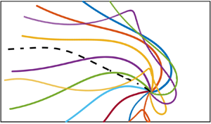
The resulting displacement patterns are shown in figure 4. Panel (a) presents simulations performed with  $W = 2$,
  ${v_{max}} = 25$ and
  $\varphi = 0,{\rm \pi} \textrm{/}6,2{\rm \pi} \textrm{/}6, \ldots ,11{\rm \pi} \textrm{/}6$. Each experiment in figure 4 was extended in time until the absolute displacement
  $\Delta R = \sqrt {\Delta {X^2} + \Delta {Y^2}} $ exceeded
  $\varDelta {R_{max}} = 50$. All vortices eventually evolve to the predominantly westward propagation with speeds close to the preferred migration rate (3.3). During the final stages of experiments, defined here as the last 20% of the integration periods, the meridional/zonal speed ratios
  $|{V/U} |$ range from 0.0032 to 0.0647, and
  $|{1 + U} |$ from 0.07 to 0.20. However, the initial conditions clearly affect the evolution of self-propagating vortices for extended periods. This influence becomes evident when their trajectories are compared to the track of the corresponding axisymmetric vortex, indicated by the dashed curve in figure 4(a). Of particular interest are the instances of eastward displacement, which can be as large as
  $\Delta X\sim 30$ – the length scale that is dimensionally equivalent to
  ${\sim} 1000\;\textrm{km}$.

Figure 4. Trajectories of vortices constructed using the Gaussian basic state for (a)  $(W,{v_{max}}) = (2,25)$, (b)
  $(W,{v_{max}}) = (1,25)$, (c)
  $(W,{v_{max}}) = (4,25)$ and (d)
  $(W,{v_{max}}) = (2,100)$. In all simulation sets, the launch angles are
  $\varphi = 0,{\rm \pi} \textrm{/}6,2{\rm \pi} \textrm{/}6, \ldots ,11{\rm \pi} \textrm{/}6$. Dashed curves represent tracks of the initially axisymmetric vortices. Different colours are used to help distinguish individual trajectories.
Panel (b) shows the analogous series of simulations performed with a relatively low target velocity  $(W = 1)$. As expected, this reduction substantially limited the long-term effect of initial non-axisymmetric perturbations. The increase in the target speed to
  $W = 4$ in panel (c), on the other hand, dramatically increases the ability of vortices to self-propagate. Six out of twelve vortices maintained their predominantly eastward movement throughout the entire experiment, thereby overcoming the opposing tendency of the centre-of-mass propagation (2.2).
Finally, panel (d) examines the ramifications of increasing the vortex strength. These simulations were performed for  ${v_{max}} = 100$ and
  $W = 2$. Despite the fourfold difference in
  ${v_{max}}$, the patterns of trajectories in (a) and (d) are qualitatively similar. This indicates that the ability of vortices to self-propagate is not particularly sensitive to the strength of their axisymmetric components. In this regard, it should be noted that the values of
  ${v_{max}}$ used for the calculations in figure 4 are broadly representative of coherent eddies in the ocean. For instance, the historical census of long-lived oceanic vortices (Olson Reference Olson1991) lists 35 well-studied examples with azimuthal velocities ranging from 0.22 to 2 m s−1. For typical oceanic parameters (3.1), this range translates to the non-dimensional velocities of
  $22 \lt {v_{max}} \lt 200$.
3.2. Zero angular momentum vortices
The second type of solutions considered in this study is that of zero angular momentum vortices. Such solutions are particularly interesting because they do not satisfy the conditions of the centroid theorem (2.2). Thus, a priori, one expects to find a wider range of migration rates and enhanced self-propagation tendencies amongst zero angular momentum eddies. These vortices are modelled in our study using the double-Gaussian streamfunction
 \begin{equation}{\psi _0} ={-} A{a_1}\,\textrm{exp}( - {a_1}{r^2}) + A{a_2}\,\textrm{exp}( - {a_2}{r^2}),\end{equation}
which satisfies the zero angular momentum condition (2). However, to use the double-Gaussian pattern, we must first identify relatively stable solutions, which do not disintegrate in simulations. Extensive exploration of the parameter space revealed that the double-Gaussian vortices tend to become more stable when  ${a_1}$ and
  ${a_2}$ are assigned dissimilar values. Since no instances of vortex fragmentation occurred in simulations performed with
  $({a_1},{a_2}) = (2,0.4)$, these parameters are used in all following experiments. The azimuthal velocity profile of the double-Gaussian vortex is shown in figure 5, along with its Gaussian counterpart. While qualitatively similar, the double-Gaussian profile is characterized by a slight reversal of the velocity in the vortex periphery
  $(r \gt 1.4)$.

Figure 5. The radial patterns of the azimuthal velocity  ${v_0}(r)$ in the Gaussian (dashed curve) and double-Gaussian (solid curve) vortices.
As previously, we use the optimization procedure (§ 2.2) to construct non-axisymmetric perturbations for given target propagation velocity values. These perturbations are then superimposed on the symmetric state (3.10) and used as an initial condition for calculations shown in figure 6. Panel (a) shows a series of experiments performed with  $W = 2$ and
  ${v_{max}} = 25$. The salient feature of these simulations is the ability of vortices to maintain the predominantly eastward course if their initial drift is eastward. Such persistence is seen even when the target speed is reduced to
  $W = 1$ in figure 6(b). An interesting aspect of high-speed experiments
  $(W = 4)$ is the nearly bi-modal pattern of vortex tracks. All trajectories in figure 6(c) are tightly grouped around two well-defined routes, westward and eastward. The increase in the eddy intensity to
  ${v_{max}} = 100$ (figure 6d) has a limited impact on the motion patterns (cf. figure 6a) and is reflected most notably in larger northward displacements of the eastward-propagating vortices.

Figure 6. The same as figure 4 but for the double-Gaussian basic state.
Figure 7 examines in greater detail two representative examples of zero angular momentum vortices. The eastward-propagating case  $(\varphi = 0)$ is illustrated in panels (a–e) and the westward example
  $(\varphi = {\rm \pi})$ is in (f–j). Although both experiments were performed using
  $W = 2$ and
  ${v_{max}} = 25$, they reveal considerably different dynamics and evolutionary patterns. The eastward-propagating vortex rapidly deviates from its initial course and by
  $t = 5$ starts moving to the north-east (figure 7b). At this stage, the vortex undergoes a substantial reorganization of its PV field. Negative PV accumulates in the south-east region of the vortex, forming a strongly asymmetric dipole. The resulting structure eventually settles into a predominantly eastward motion pattern (figure 7c,d) along the
  $y = 10$ latitude. Its zonal migration is accompanied by periodic meridional excursions of decreasing magnitude.

Figure 7. Numerical simulations initiated by the zero angular momentum (double-Gaussian) vortices. Panels (a–e) present the evolution of the eastward-propagating vortex  $(\varphi = 0)$, and the westward example
  $(\varphi = {\rm \pi})$ is in (f–j). The instantaneous PV patterns in each experiment are shown at
  $t = 0,\;5,\;15,\;25$ and 35. Both simulations were performed with
  $(W,{v_{max}}) = (2,25)$. Only the parts of computational domains containing the vortex are shown.
These oscillations and their eventual stabilization can be interpreted as a ramification of the Lagrangian conservation of the total PV (3.6). This principle implies that any northward displacement – and the associated increase in the planetary PV component – is necessarily accompanied by the decrease in the fluid PV (q). Thus, when an approximately balanced vortex that is travelling predominantly eastward drifts to the north, the decrease in q induces anticyclonic perturbation. As a result, the entire structure tends to rotate clockwise, and the vortex turns right, eventually reversing its northward drift. Applying similar arguments to the vortex moving south-east, we conclude that it should turn left and reverse its southward displacement. This negative feedback leads to the directional stabilization of the vortex trajectory and phase locking of its dipolar component into the orientation required for eastward propagation. It is interesting to note that directional stabilization was originally discovered in the context of dipolar eddy models (Zabusky & McWilliams Reference Zabusky and McWilliams1982). Subsequently, the tendency of approximately symmetric dipoles to evolve into eastward-propagating structures has been explored using simulations (Hesthaven, Lynov & Nycander Reference Hesthaven, Lynov and Nycander1993; Sutyrin et al. Reference Sutyrin, Hesthaven, Lynov and Rasmussen1994), laboratory experiments (Kloosterziel, Carnevale & Phillippe Reference Kloosterziel, Carnevale and Phillippe1993) and was recently identified in the ocean using satellite altimeter data (Hughes & Miller Reference Hughes and Miller2017). The present investigation, however, demonstrates that the directional stabilization of eastward propagation can also occur for quasi-monopolar vortices.
The motion pattern of the westward-propagating vortex in (f–j) is more regular and predictable. The vortex largely retains its initial structure and uniform motion pattern throughout the entire simulation. Perhaps the only qualitative difference between this experiment and its finite angular momentum counterpart in figure 3 is a larger northward drift in figure 7.
4. The mechanisms of self-propagation on the beta-plane and the f-plane
The beta-plane calculations in § 3 reveal that the initial asymmetries of coherent vortices can exert a strong and prolonged influence on their dynamics and motion patterns. This observation prompts the question of whether similar effects can also occur on the f-plane  $(\beta = 0)$. An intriguing aspect of this problem concerns the largely bi-modal evolutionary patterns of the beta-plane vortices (figures 4 and 6), which exhibit either predominantly westward or eastward long-term propagation. Since the f-plane model is directionally invariant, it may represent dissimilar self-propagation mechanisms and tendencies. This possibility is explored by performing simulations with the f-plane equivalent-barotropic model
 \begin{equation}\frac{\partial }{{\partial t}}\left( {{\nabla^2}\psi - \frac{\psi }{{R_d^2}}} \right) + J(\psi ,{\nabla ^2}\psi ) = \nu {\nabla ^4}\psi ,\end{equation}
which differs from the governing equation of the beta-plane model (2.1) by the exclusion of the beta term  $\partial \psi /\partial x$. All other parameters in the following f-plane experiments are identical to their beta-plane counterparts. The following analysis is couched in terms of constraints on the propagation speed posed by the centroid theorem (§ 2).
As previously (§ 3), the f-plane experiments were initialized by the superposition of the axisymmetric Gaussian vortex  $({v_{max}} = 25)$ and the optimal perturbations computed for the desired propagation speeds (W) and launch angles
  $(\varphi )$. The salient differences in the evolution of these f-plane vortices and their beta-plane counterparts are illustrated in figure 8. These simulations exemplify two distinct regimes, characterized by strong and weak initial perturbations. The strong perturbation experiments were performed with
  $(W,\varphi ) = (4,0)$ and are presented in figure 8(a,c) for the beta-plane and f-plane models, respectively. For the weak perturbation runs, we used
  $(W,\varphi ) = (2,{\rm \pi} )$ and the results are shown in figures 8(b) and 8(d).

Figure 8. Comparison of the beta-plane and f-plane simulations. The beta-plane experiments are presented in (a) and (b) for  $(W,\varphi ) = (4,0)$ and
  $(W,\varphi ) = (2,{\rm \pi} )$, respectively; their f-plane counterparts are shown in (c) and (d), respectively. In the left panels, the speeds of the vortex centre U (black curves) and its centroid
  $\textrm{d}{x_c}/\textrm{d}t$ (red curves) are plotted as functions of time. The right panels present the temporal records of the angular momentum
  $({I_\psi })$.
On the beta-plane, strong perturbations with the predominantly eastward launch angles (figure 4c) produce the persistent drift of vortices in the positive x-direction  $(U \gt 0)$. This tendency appears to be at odds with the centroid theorem (§ 2), which predicts the centre-of-mass speed of
  $U ={-} 1$. Thus, the position of the vortex centre – as determined here from the best Gaussian fit to its streamfunction – and of its centroid can separate considerably in time. To rationalize this peculiar result, we introduce the following operational definition for the coordinates of the centroid, which can be conveniently diagnosed from simulations
 \begin{equation}{x_c} = \frac{{\iint_S {x(\psi - {\psi _\infty })\,\textrm{d}x\,\textrm{d}y} }}{{\iint_S {(\psi - {\psi _\infty })\,\textrm{d}x\,\textrm{d}y} }},\quad {y_c} = \frac{{\displaystyle\iint_S {y(\psi - {\psi _\infty })\,\textrm{d}x\,\textrm{d}y} }}{{\displaystyle\iint_S {(\psi - {\psi _\infty })\,\textrm{d}x\,\textrm{d}y} }},\end{equation}
where S represents the circular area of radius R surrounding the vortex centre and  ${\psi _\infty }$ is the streamfunction average along its boundary
  $(r = R)$. In the present calculations (figure 8), we use
  $R = {L_x}/4 = 7.5$. This moderately large value is chosen to ensure that (i) R greatly exceeds the vortex size, which is one of the assumptions of the centroid theorem, and (ii) R is considerably less than the extent of the computational domain, which limits the potential contamination of the results by the periodic boundary conditions.
The left panel of figure 8(a) presents the speed of the vortex centre (U) and of its centroid  $(\textrm{d}{x_c}/\textrm{d}t)$ as functions of time. The latter quantity was evaluated using (4.2). The most striking feature of this calculation is the dramatic difference in the behaviour of the vortex centre and its centroid. The centre propagates in a natural and predictable manner, maintaining its predominantly eastward course with speed gradually decreasing in time from its initial value of
  $U = 4$. The motion of the centroid, on the other hand, is characterized by the erratic large-amplitude excursions in all directions – the pattern which appears to be decoupled from the motion of the vortex itself. This counterintuitive result can be rationalized by examining the evolution of the vortex angular momentum
 \begin{equation}{I_\psi } ={-} \iint_S {(\psi - {\psi _\infty })\,\textrm{d}x\,\textrm{d}y} ,\end{equation}
which is plotted in the right panel of figure 8(a). The angular momentum exhibits extremely high levels of temporal variability, marked by numerous changes in its sign. Each time  ${I_\psi }$ approaches zero, the expressions in (4.2) become singular, which leads to the rapid and unbounded increase in the centroid displacement.
The relatively fast oscillations of  ${I_\psi }$ are modulated on longer time scales, which systematically reduces the magnitude of angular momentum in time. The implications of this tendency for vortex propagation are profound. The finite value of angular momentum is the necessary condition for the applicability of the centroid theorem (§ 2). Thus, the observed expulsion of angular momentum from the area surrounding the vortex removes the severe constraint on its propagation velocity posed by the centroid theorem. This mechanism makes it possible for the vortex to maintain a drift rate that is very different from the speed of long Rossby waves.
The expulsion of angular momentum in the strong perturbation experiments on the beta-plane can be attributed to the northward displacement of the vortex. The Lagrangian conservation of the total PV (3.6) implies that this displacement, which increases the planetary PV component, is accompanied by the decrease in the fluid PV (q). The associated spin-down of the vortex leads to the reduction of its angular momentum. This hypothesis is supported by the apparent anticorrelation of the meridional displacement  $({y_c})$ and the angular momentum
  $({I_\psi })$, with the strongly negative correlation coefficient of
  ${r_{cor}} ={-} 0.80$ obtained for the experiment in figure 8(a). It should be emphasized that this mechanism of expulsion depends principally on the beta-effect and is inapplicable to the f-plane experiments that will be analysed shortly.
Figure 8(b) presents an example of the weakly perturbed vortex on the beta-plane. After its release at the launch angle of  $\varphi = {\rm \pi}$, the vortex continues to propagate westward throughout the entire simulation. The initial drift rate
  $(U ={-} 2)$ is higher than the speed predicted by the centroid theorem
  $(U ={-} 1)$ but not dramatically so. The dynamics of such weakly forced systems is very dissimilar to that of strongly perturbed vortices (cf. figure 8a). The drift rate of the vortex in figure 8(b) gradually and uneventfully reduces to the centroid speed. The angular momentum remains large throughout the simulation, and therefore the vortex eventually conforms to the constraints on its drift rate placed by the centroid theorem.
Finally, we turn our attention to the f-plane counterparts of the foregoing simulations. In the absence of the beta-effect, the centroid theorem predicts  $U = 0$. Thus, the question arises whether some initial vortical states could still exhibit strong self-propagation tendencies, as seen previously in several beta-plane experiments (e.g. figure 4c). Figures 8(c) and 8(d) present the evolution of the strongly
  $(W = 4)$ and weakly
  $(W = 2)$ perturbed f-plane vortices, respectively. In both cases, the vortices oscillate around their points of origin with very limited net displacement. Figure 9 presents the vortex trajectory in the strongly perturbed
  $(W = 4)$ experiment, which was extended in time for
  $t = 1000$ units. During the entire period, the vortex propagated in a circuitous manner, accumulating the net displacement of only
  ${L_{net}} = 10.1$. This motion pattern is remarkably inefficient, particularly considering that the entire length of the vortex trajectory exceeds its net displacement by two orders of magnitude:
  ${L_{tr}} = 977.0$.

Figure 9. The trajectory of the vortex in the f-plane experiment performed with  $(W,\varphi ) = (4,0)$. The simulation was extended in time for
  $t = 1000$ non-dimensional units. The red (green) dot represents the starting (ending) point.
The inability of vortices to self-propagate over large distances on the f-plane can be attributed to the lack of effective mechanisms for the expulsion of angular momentum. On the beta-plane, the systematic expulsion (figure 8a) was aided by the meridional drift and the associated change of planetary vorticity. However, such a change does not occur on the f-plane. The angular momentum in the f-plane experiments still exhibits substantial temporal variability (figure 8c,d) but it is fundamentally transient in nature. Despite the presence of rapid oscillations in time series of  ${I_\psi }$, the mean values of angular momentum remain fairly uniform in time. For instance, the averages of
  ${I_\psi }$ over the intervals
  $0 \lt t \lt 100$ and
  $100 \lt t \lt 200$ differ by less than 15% in both f-plane experiments (figure 8c,d). As a result, all f-plane vortices passively succumb to the restrictions on self-propagation imposed by the centroid theorem.
5. Reduced-dynamics model
The intriguing behaviour of self-propagating vortices revealed by the foregoing simulations motivates an attempt to rationalize some of the observed features using more transparent reduced-dynamics models. The model considered in this study is analogous to those developed by Sutyrin et al. (Reference Sutyrin, Hesthaven, Lynov and Rasmussen1994), Reznik & Dewar (Reference Reznik and Dewar1994) and Sutyrin and Flierl (Reference Sutyrin and Flierl1994) and it is briefly described below.
The following calculations are performed in the frame of reference moving with the speed of the vortex  $({u_q},{v_q})$. To be specific, the origin of the coordinate system is placed at the location of its PV extremum. For cyclonic eddies considered in the present study, this location corresponds to the maximum of
  $q(x,y)$. In the new coordinate system, the equivalent-barotropic equation (2.7) becomes
 \begin{equation}\frac{{\partial q}}{{\partial t^{\prime}}} - {u_q}\frac{{\partial q}}{{\partial x^{\prime}}} - {v_q}\frac{{\partial q}}{{\partial y^{\prime}}} + J(\psi ,q) + \frac{{\partial \psi }}{{\partial x^{\prime}}} = {\nu _{nd}}{\nabla ^4}\psi ,\end{equation}
where  $t^{\prime} = t$,
  $x^{\prime} = x - {u_q}t$ and
  $y^{\prime} = y - {v_q}t$. The streamfunction and PV fields are then separated into the axisymmetric components (
 ${\psi _0}$ and
  ${q_0}$) and perturbations (
 $\psi ^{\prime}$ and
  $q^{\prime}$). We assume that
  $q^{\prime}$,
  $\psi ^{\prime}$,
  ${u_q}$ and
  ${v_q}$ are order-one quantities that are much less than the axisymmetric flow fields
  ${\psi _0} \gg 1$ and
  ${q_0} \gg 1$ in the vortex interior. The equivalent-barotropic equation (5.1) is then linearized about the dominant axisymmetric pattern. The linear character of the resulting system makes it possible to analyse the evolution of dipolar perturbations without taking higher azimuthal harmonics into account. Thus, the PV and streamfunction fields are represented by a superposition of the axisymmetric component, which does not change in time, and the first azimuthal harmonic
 \begin{equation}\left. {\begin{array}{c@{}} {\psi = {\psi_0} + {\psi_c}\cos \theta + {\psi_s}\sin \theta ,}\\ {q = {q_0} + {q_c}\cos \theta + {q_s}\sin \theta ,} \end{array}} \right\}\end{equation}
where
 \begin{equation}{q_{c,s}} = \frac{{{\partial ^2}{\psi _{c,s}}}}{{\partial {r^2}}} + \frac{1}{r}\frac{{\partial {\psi _{c,s}}}}{{\partial r}} - \left( {\frac{1}{{{r^2}}} + 1} \right){\psi _{c,s}},\end{equation}
and the continuity of PV demands that
 \begin{equation}{q_c} = {q_s} = 0\quad \textrm{at}\;r = 0.\end{equation}
 The truncated series (5.2) are substituted into the linearization of (5.1) and their  $\textrm{cos}\,\theta $ and
  $\textrm{sin}\,\theta $ components are isolated, which results in
 \begin{equation}\left. {\begin{array}{c@{}} {\dfrac{{\partial {q_c}}}{{\partial t}} = {u_q}\dfrac{{\partial {q_0}}}{{\partial r}} - \dfrac{1}{r}\dfrac{{\partial {\psi_0}}}{{\partial r}}{q_s} + \dfrac{1}{r}\dfrac{{\partial {q_0}}}{{\partial r}}{\psi_s} - \dfrac{{\partial {\psi_0}}}{{\partial r}} + {\nu_{nd}}{{\left( {\dfrac{{{\partial^2}}}{{\partial {r^2}}} + \dfrac{1}{r}\dfrac{\partial }{{\partial r}} - \dfrac{1}{{{r^2}}}} \right)}^2}{\psi_c},}\\ {\dfrac{{\partial {q_s}}}{{\partial t}} = {v_q}\dfrac{{\partial {q_0}}}{{\partial r}} + \dfrac{1}{r}\dfrac{{\partial {\psi_0}}}{{\partial r}}{q_c} - \dfrac{1}{r}\dfrac{{\partial {q_0}}}{{\partial r}}{\psi_c} + {\nu_{nd}}{{\left( {\dfrac{{{\partial^2}}}{{\partial {r^2}}} + \dfrac{1}{r}\dfrac{\partial }{{\partial r}} - \dfrac{1}{{{r^2}}}} \right)}^2}{\psi_s}.} \end{array}} \right\}\end{equation}
Since  $r = 0$ is defined as the location of the PV maximum,
 \begin{equation}{\left. {\frac{{\partial {q_c}}}{{\partial r}}} \right|_{r = 0}} = {\left. {\frac{{\partial {q_s}}}{{\partial r}}} \right|_{r = 0}} = 0.\end{equation}
This, in turn, makes it possible to determine the eddy propagation velocity by considering the leading-order balance of (5.5) in the limit  $r \to 0$ and assuming that
  ${\nu _{nd}} \ll 1$
 \begin{equation}\left. {\begin{array}{c@{}} {{u_q} = \mathop {\lim }\limits_{r \to 0} \left( {{{\dfrac{{\partial {\psi_0}}}{{\partial r}}} / {\dfrac{{\partial {q_0}}}{{\partial r}} - \dfrac{{{\psi_s}}}{r}}}} \right),}\\ {{v_q} = \mathop {\lim }\limits_{r \to 0} \left( {\dfrac{{{\psi_c}}}{r}} \right).} \end{array}} \right\}\end{equation}
The system (5.3), (5.5) and (5.7) is solved using the spectral method based on the first-order Hankel transform in r
 \begin{equation}\tilde{C}(s) = {H_1}\{ C(r)\} \equiv \int_0^\infty {C(r){J_1}(sr)r\,\textrm{d}r} .\end{equation}
The Hankel transform allows us to conveniently evaluate and invert the Laplace and Helmholtz operators in polar coordinates using the identity
 \begin{equation}{H_1}\left\{ {\frac{{{\partial^2}C}}{{\partial {r^2}}} + \frac{1}{r}\frac{{\partial C}}{{\partial r}} - \frac{C}{{{r^2}}}} \right\} ={-} {s^2}\tilde{C}.\end{equation}
The numerical algorithm employs the discrete Hankel transforms (forward and inverse) as a means of converting variables between physical and spectral spaces. The physical interval  $0 \lt r \lt R$ is discretized using
  ${n_r}$ grid points. In all presented experiments
  $(R,{n_r}) = ({15,512} )$, and the temporal integration is performed using the fourth-order Runge–Kutta scheme.
As previously (§ 3), we start the analysis by computing the optimal perturbation for a given target velocity  $(U,V)$. The perturbation PV values at grid points
  ${q_c}({r_i})$ and
  ${q_s}({r_i})$, where
  $i = 1,2, \ldots ,{n_r}$, represent the input variables for the optimization module that minimizes the tendency norm (2.14). The resulting optimal perturbations are then used as initial conditions for temporal integrations of the reduced-dynamics system (5.3), (5.5) and (5.7). Figure 10 presents the trajectories computed in this manner for the finite angular momentum Gaussian vortex (3.2). The striking difference between this set of experiments and their nonlinear counterparts in figure 4 is the absence of any substantial eastward displacements in figure 10. The other notable feature of reduced-dynamics simulations is the lack of complexity and small-scale variability in vortex pathways that is evident in the equivalent-barotropic simulations (figure 4). The trajectories in figure 10 follow regular predominantly westward routes, not unlike the tracks of initially unperturbed vortices. Thus, the erratic character of trajectories in the equivalent-barotropic model – realized for particularly strong perturbations (figure 4) – can reflect the control of the dipolar mode by fundamentally nonlinear processes. The inability of the reduced model to capture pathways of non-axisymmetric eddies stands in stark contrast to its fairly accurate representation of the trajectories of axisymmetric vortices (dashed curves in figures 4 and 10). Overall, the results in figure 10 indicate that the variation in the magnitude and direction of target velocity in the reduced-dynamics model mostly affects the net meridional displacements of vortices, but not much else.

Figure 10. The reduced-dynamics propagation model. Trajectories of Gaussian vortices are presented for (a)  $(W,{v_{max}}) = (2,25)$, (b)
  $(W,{v_{max}}) = (1,25)$, (c)
  $(W,{v_{max}}) = (4,25)$ and (d)
  $(W,{v_{max}}) = (2,100)$. In all simulation sets, the launch angles are
  $\varphi = 0,{\rm \pi} /6,2{\rm \pi} /6, \ldots ,11{\rm \pi} /6$. Dashed curves represent tracks of the initially axisymmetric vortices.
Finally, we present (figure 11) a series of calculations performed with the double-Gaussian, zero angular momentum vortex (3.10). These experiments reveal a richer array of motion patterns than in figure 10. Trajectories are more dispersed and there are even some instances of eastward displacements, particularly for large target velocities (e.g.  $W = 4$ case in figure 11c). Nevertheless, qualitative differences between solutions of (5.5) and full equivalent-barotropic simulations (figure 6) are apparent. The reduced-dynamics solutions are less chaotic and more predictable, resulting in individual trajectories that generally follow the tracks of the initially axisymmetric vortices. These differences underscore the inherent limitations of the linear model (5.5) in representing the dynamics of self-propagation. This model excludes potentially significant nonlinear mechanisms, such as the phase locking of the first azimuthal mode that can lead to substantial eastward displacements of vortices (e.g. figure 7a–e).

Figure 11. The same as figure 10 but for the double-Gaussian basic state.
6. Discussion and conclusions
This study explores the dynamics and displacement patterns of quasi-monopolar vortices under the combined influence of their initial asymmetries and the beta-effect. The key question – whether slight structural imperfections could have long-lasting effects on the evolution of predominantly axisymmetric vortices – was answered affirmatively. The ability of coherent vortices to retain the memory of weak initial perturbations greatly exceeded our intuitive expectations. The impact of such perturbations in simulations lasts for months, and the pathways of perturbed vortices deviate from the trajectories of their axisymmetric counterparts by hundreds of kilometres. Perhaps the most dramatic examples of self-propagation are represented by vortices persistently moving to the east. In these cases, the initially introduced asymmetries efficiently offset the natural tendency of coherent vortices to drift westward due to the meridional gradient of planetary vorticity. The mechanism of self-propagation in this regime involves the expulsion of the angular momentum from the area surrounding the vortex (§ 4), which effectively removes the severe constraint on its drift rate imposed by the centroid theorem (§ 2).
It should be mentioned that the possibility of active control of vortex displacement patterns by their asymmetric components has long been recognized by the community. For instance, the self-propagation dynamics is explicitly represented in the exact modon-with-the-rider solutions (Berestov Reference Berestov1979; Flierl et al. Reference Flierl, Larichev, McWilliams and Reznik1980; Kizner, Berson & Khvoles Reference Kizner, Berson and Khvoles2003). These structures can propagate zonally – westward or eastward – with speeds that are ultimately determined by the strength of modons. However, more quantitative assessments of self-propagation tendencies based on such solutions are harder to come by. The key obstacle is the strong instability of oceanographically relevant configurations consisting of dominant riders and relatively weak modons (Swenson Reference Swenson1987). In the present study, this complication is bypassed by developing stable analogues of the modon-with-the-rider solutions. The proposed algorithm assumes a relatively stable axisymmetric pattern and then determines optimal perturbations that uniformly displace the entire structure with a given target velocity. While the resulting solutions may not be exact, they are sufficiently robust to be used as initial states in numerical experiments on self-propagation.
The ability of coherent vortices to persistently self-propagate due to initial asymmetries can be attributed to fundamentally nonlinear processes. The term ‘nonlinear’ in this context pertains to the beta-induced evolution of non-axisymmetric components and their self-interactions. This somewhat counterintuitive conclusion is based on calculations performed using the linearized model of propagation (§ 5), which assumes that the axisymmetric circulation of a vortex greatly exceeds the dipolar perturbation. Such an assumption is reasonable, conventional and appears to be consistent with the design of numerical simulations (§ 3). Nevertheless, the linear model substantially underestimates the sensitivity of the long-term vortex evolution to the initially introduced perturbations. For instance, the linear calculations cannot represent large eastward displacements that are seen in the more general equivalent-barotropic simulations.
This work can be further extended by systematically increasing the complexity and realism of model configurations. The minimal design of the present model is intentional. The simplicity and convenience of the equivalent-barotropic framework helped to identify the essential physics at play and to develop effective algorithms for the analysis of self-propagation. However, the inclusion of the effects that are not captured by the equivalent-barotropic model is known to improve the representation of the vortex dynamics realized in laboratory experiments and the ocean (e.g. Zavala Sansón and van Heijst Reference Zavala Sansón and van Heijst2002; Zavala Sansón Reference Zavala Sansón2019). Thus, the investigations of more general systems (multilayer, non-quasi-geostrophic or continuously stratified) are expected to reveal new and richer dynamics. For instance, an interesting question arises regarding the nonlinear coupling of baroclinic and barotropic vertical modes, and its impact on the vortex drift rate. Such coupling could play a significant role in fully baroclinic configurations but is not reflected in the equivalent-barotropic system (2.1).
The inclusion of background large-scale circulation patterns in the model represents yet another exciting avenue for future explorations of self-propagation. In particular, the presence of a baroclinic shear would likely affect the dynamics of self-propagation. The vertical shear represents a source of the available potential energy that can be transferred to the vortex (e.g. Sutyrin and Radko Reference Sutyrin and Radko2021) and thereby affect its motion pattern. Strong, baroclinically unstable shears are also responsible for much of mesoscale variability in the ocean, and the interaction of coherent vortices with the resulting disorganized eddy field may alter their speed and evolution. The final item on our wish list is the enhancement of the predictive skills of the reduced-dynamics models (§ 5) in representing self-propagation. This can be achieved, for instance, by incorporating various dynamically significant higher-order corrections to the linear vortex theory (e.g. Reznik, Grimshaw & Benilov Reference Reznik, Grimshaw and Benilov2000).
Acknowledgements
The author thanks Drs R. Versicco, J. Brown, G. Sutyrin and the anonymous reviewers for helpful comments.
Funding
This work was supported by the National Science Foundation (grant OCE 1828843) is gratefully acknowledged.
Declaration of interests
The author reports no conflict of interest.


