2 Theory and methods

The mathematical inviscid, adiabatic framework of strain-induced frontogenesis (Hoskins & Bretherton Reference Hoskins and Bretherton1972; Hoskins Reference Hoskins1982; Shakespeare & Taylor Reference Shakespeare and Taylor2013) describes the formation of fronts when strained by a geostrophically balanced strain flow, such as mesoscale eddies (or synoptic weather in the atmospheric case). Shakespeare & Taylor (Reference Shakespeare and Taylor2013) (hereafter Reference Shakespeare and TaylorST13) generalized the mathematical framework by Hoskins & Bretherton (Reference Hoskins and Bretherton1972) (hereafter Reference Hoskins and BrethertonHB72), to include fronts generated by an unbalanced flow. We follow the formulation presented in Reference Shakespeare and TaylorST13 for a rotating fluid in Cartesian coordinates in an incompressible, hydrostatic, Boussinesq flow on an untilted $f$-plane. In the limit of Reference Hoskins and BrethertonHB72, the equations reduce to the semi-geostrophic equations suited for describing the early stages of strain-induced frontogenesis. Eddy viscosity and diffusivity are added as new forcing terms, but otherwise this treatment and notation follows Reference Shakespeare and TaylorST13.

The velocity and pressure terms are written as

(2.1)$$\begin{eqnarray}\left.\begin{array}{@{}c@{}}U=\bar{U}+u(x,z,t)=-\unicode[STIX]{x1D6FC}x+u(x,z,t),\\ V=\bar{V}+v(x,z,t)=\unicode[STIX]{x1D6FC}y+v(x,z,t),\\ W=0+w(x,z,t),\\ \displaystyle P=\bar{P}+p(x,z,t)=\unicode[STIX]{x1D70C}_{0}\left[-\unicode[STIX]{x1D6FC}^{2}\frac{(x^{2}+y^{2})}{2}+f\unicode[STIX]{x1D6FC}xy\right]+p(x,z,t),\\ B=0+b(x,z,t),\end{array}\right\}\end{eqnarray}$$

where $\bar{U},\bar{V},\bar{P}$ are the background balanced, horizontal large-scale deformation fields and the associated pressure field respectively. The reference density is $\unicode[STIX]{x1D70C}_{0}$, $f$ is the Coriolis parameter and $u,v,w,p,b$ are the laminar frontogenetic velocity, pressure and buoyancy fields. As appropriate for a mixed layer, upper ocean problem, weak background buoyancy stratification is assumed, so the background pressure field can be thought to occur primarily by sea surface height anomalies. The laminar frontogenetic fields are assumed to be nearly independent of the along-front direction $y$, so only $\bar{V}$ and $\bar{P}$ vary in $y$. The strain rate $\unicode[STIX]{x1D6FC}$ is taken as a constant, an approximation valid when $\unicode[STIX]{x1D6FC}$ represents much larger-scale features, such as mesoscale eddies, that do not vary over the confluence region of the submesoscale front in question. Furthermore, the semi-geostrophic approximation requires that $\unicode[STIX]{x1D6FC}/f\ll 1$, which can also be described as a small Rossby number approximation. Note that $y$-invariance presumes that the laminar frontogenetic variables represent laminar perturbations to the background flow. All turbulent contributions will be assumed to be scale separated from these laminar flows, and thus treated via parameterization: here eddy viscosity and diffusivity are the explicit parameterization forms carried through the analysis, although generalizations are readily handled with the same methodology. To review, the flow is decomposed as a sum of background (capital letters), laminar frontogenetic (lower case) and turbulent (parameterized so not explicitly part of $u,v,w,b,p$, and either frontogenetic or frontolytic) pieces.

It is useful to introduce a vector streamfunction, with a geostrophic (vertical) component $\unicode[STIX]{x1D6F7}$ (sometimes called ‘velocity potential’), and an ageostrophic (along-front) component $\unicode[STIX]{x1D6F9}$. The geostrophic streamfunction component is related to the pressure and horizontal geostrophic velocities by dividing into background and laminar frontogenetic contributions $\unicode[STIX]{x1D6F7}=\bar{\unicode[STIX]{x1D719}}+\unicode[STIX]{x1D719}(x,z,t)$,

(2.2a,b)$$\begin{eqnarray}\displaystyle \bar{\unicode[STIX]{x1D719}}=\frac{\bar{P}}{\unicode[STIX]{x1D70C}_{0}f}+\unicode[STIX]{x1D6FC}^{2}\frac{(x^{2}+y^{2})}{2f}=\unicode[STIX]{x1D6FC}xy,\quad \unicode[STIX]{x1D719}(x,z,t)=\frac{p(x,z,t)}{\unicode[STIX]{x1D70C}_{0}f}, & & \displaystyle\end{eqnarray}$$

(2.3a-d)$$\begin{eqnarray}\displaystyle \frac{\unicode[STIX]{x2202}\bar{\unicode[STIX]{x1D719}}}{\unicode[STIX]{x2202}y}=-\bar{U},\quad \frac{\unicode[STIX]{x2202}\bar{\unicode[STIX]{x1D719}}}{\unicode[STIX]{x2202}x}=\bar{V},\quad \frac{\unicode[STIX]{x2202}\unicode[STIX]{x1D719}}{\unicode[STIX]{x2202}y}=-u_{g}=0,\quad \frac{\unicode[STIX]{x2202}\unicode[STIX]{x1D719}}{\unicode[STIX]{x2202}x}=v_{g}. & & \displaystyle\end{eqnarray}$$

While the ageostrophic, or ‘overturning circulation’, streamfunction component is related to the ageostrophic laminar frontogenetic velocities $\unicode[STIX]{x1D6F9}=0+\unicode[STIX]{x1D713}(x,z,t)$,

(2.4a,b)$$\begin{eqnarray}\displaystyle \frac{\unicode[STIX]{x2202}\unicode[STIX]{x1D713}}{\unicode[STIX]{x2202}z}=u_{a},\quad -\frac{\unicode[STIX]{x2202}\unicode[STIX]{x1D713}}{\unicode[STIX]{x2202}x}=w=w_{a}. & & \displaystyle\end{eqnarray}$$

Please note that to be consistent with Reference Shakespeare and TaylorST13, we follow the left-hand rule definition for the streamfunction, rather than the right-hand rule as defined in Reference Hoskins and BrethertonHB72. Furthermore, here the term ‘secondary’ is avoided as a description of the overturning circulation, as it is easily confused with the order of the perturbation analysis. Likewise, the phrase ‘laminar frontogenetic’ is preferred over the more common ‘perturbation’ velocity because it is easily confused with terms involved in the perturbation method. As in Reference Hoskins and BrethertonHB72, the leading-order along-front laminar frontogenetic velocities are purely geostrophic ($v\equiv v_{g}$), and the cross-front laminar frontogenetic velocity is a combination of geostrophic and ageostrophic components ($u=u_{g}+u_{a}$). The background straining velocity is given by $\bar{\unicode[STIX]{x1D719}}$ alone.

Similar to Reference Shakespeare and TaylorST13, the governing equations for the two-dimensional laminar frontogenetic response to the background flow can be expanded out from the definitions above, assuming hydrostatic, laminar flow. Here we include the novel addition of an eddy diffusive flux $F(b)$ and viscous flux $F(u),F(v)$. For now, these are written in a form amenable to accommodate most present parameterizations, including spatial variation, non-local fluxes and tensor character (Large, McWilliams & Doney Reference Large, McWilliams and Doney1994; Griffies Reference Griffies1998; Fox-Kemper, Ferrari & Hallberg Reference Fox-Kemper, Ferrari and Hallberg2008; Bachman, Fox-Kemper & Bryan Reference Bachman, Fox-Kemper and Bryan2015; Bachman et al. Reference Bachman, Fox-Kemper, Taylor and Thomas2017).

(2.5a)$$\begin{eqnarray}\displaystyle & \displaystyle \frac{\text{D}u}{\text{D}t}-fv=\unicode[STIX]{x1D6FC}u-\frac{1}{\unicode[STIX]{x1D70C}_{0}}\frac{\unicode[STIX]{x2202}p}{\unicode[STIX]{x2202}x}+\unicode[STIX]{x1D735}\boldsymbol{\cdot }F(u), & \displaystyle\end{eqnarray}$$

(2.5b)$$\begin{eqnarray}\displaystyle & \displaystyle \frac{\text{D}v}{\text{D}t}+fu=-\unicode[STIX]{x1D6FC}v+\unicode[STIX]{x1D735}\boldsymbol{\cdot }F(v), & \displaystyle\end{eqnarray}$$

(2.5c)$$\begin{eqnarray}\displaystyle & \displaystyle 0=b-\frac{1}{\unicode[STIX]{x1D70C}_{0}}\frac{\unicode[STIX]{x2202}p}{\unicode[STIX]{x2202}z}, & \displaystyle\end{eqnarray}$$

(2.5d)$$\begin{eqnarray}\displaystyle & \displaystyle \frac{\text{D}b}{\text{D}t}=\unicode[STIX]{x1D735}\boldsymbol{\cdot }F(b), & \displaystyle\end{eqnarray}$$

(2.5e)$$\begin{eqnarray}\displaystyle & \displaystyle \frac{\unicode[STIX]{x2202}u}{\unicode[STIX]{x2202}x}+\frac{\unicode[STIX]{x2202}w}{\unicode[STIX]{x2202}z}=0, & \displaystyle\end{eqnarray}$$

$b$

(2.6)$$\begin{eqnarray}\frac{\unicode[STIX]{x2202}\unicode[STIX]{x1D719}}{\unicode[STIX]{x2202}z}=\frac{b}{f}.\end{eqnarray}$$

The material derivative is defined as

(2.7)$$\begin{eqnarray}\frac{\text{D}}{\text{D}t}\equiv \frac{\unicode[STIX]{x2202}}{\unicode[STIX]{x2202}t}+(u+\bar{U})\frac{\unicode[STIX]{x2202}}{\unicode[STIX]{x2202}x}+w\frac{\unicode[STIX]{x2202}}{\unicode[STIX]{x2202}z}.\end{eqnarray}$$

Equation (2.5e) will be automatically satisfied if the streamfunctions $\unicode[STIX]{x1D719}$ and $\unicode[STIX]{x1D713}$ are chosen as the prognostic variables instead of $u,v,w$.

For concreteness, we will assume in the following that the viscous and diffusive fluxes can be written as horizontal and vertical fluxes, assumed to be down gradient with constant viscosities and diffusivities

(2.8)$$\begin{eqnarray}\displaystyle & \displaystyle F(u)=\hat{x}\unicode[STIX]{x1D708}_{H}\frac{\unicode[STIX]{x2202}u}{\unicode[STIX]{x2202}x}+\hat{z}\unicode[STIX]{x1D708}_{V}\frac{\unicode[STIX]{x2202}u}{\unicode[STIX]{x2202}z}, & \displaystyle\end{eqnarray}$$

(2.9)$$\begin{eqnarray}\displaystyle & \displaystyle F(v)=\hat{x}\unicode[STIX]{x1D708}_{H}\frac{\unicode[STIX]{x2202}v}{\unicode[STIX]{x2202}x}+\hat{z}\unicode[STIX]{x1D708}_{V}\frac{\unicode[STIX]{x2202}v}{\unicode[STIX]{x2202}z}, & \displaystyle\end{eqnarray}$$

(2.10)$$\begin{eqnarray}\displaystyle & \displaystyle F(b)=\hat{x}\unicode[STIX]{x1D705}_{H}\frac{\unicode[STIX]{x2202}b}{\unicode[STIX]{x2202}x}+\hat{z}\unicode[STIX]{x1D705}_{V}\frac{\unicode[STIX]{x2202}b}{\unicode[STIX]{x2202}z}. & \displaystyle\end{eqnarray}$$

Consistent with assuming that the laminar fields do not vary in $y$, we assume that turbulent fluxes are statistically homogeneous in $y$ and thus the ${\hat{y}}$ component can be ignored. One might be tempted to suggest that molecular viscosity and diffusivity might be used here, but we will soon see that asymptotic ordering demands an upper and a lower limit on Reynolds and Péclet number, so keep in mind that these terms are intended as turbulence parameterizations.

Within the mixed layer, these fluxes are assumed to be a direct result of turbulence, whereas in the very near-surface boundary they can be matched to applied wind shear ($\unicode[STIX]{x1D70F}/\unicode[STIX]{x1D70C}_{0}$) and thermodynamic forcing ($Q$) via frictional and diabatic flux boundary conditions

(2.11a)$$\begin{eqnarray}\displaystyle & \displaystyle \frac{\unicode[STIX]{x1D70F}_{x}}{\unicode[STIX]{x1D70C}_{0}}=\hat{z}\unicode[STIX]{x1D708}_{V}\frac{\unicode[STIX]{x2202}u}{\unicode[STIX]{x2202}z}, & \displaystyle\end{eqnarray}$$

(2.11b)$$\begin{eqnarray}\displaystyle & \displaystyle \frac{\unicode[STIX]{x1D70F}_{y}}{\unicode[STIX]{x1D70C}_{0}}=\hat{z}\unicode[STIX]{x1D708}_{V}\frac{\unicode[STIX]{x2202}v}{\unicode[STIX]{x2202}z}, & \displaystyle\end{eqnarray}$$

(2.11c)$$\begin{eqnarray}\displaystyle & \displaystyle Q=\hat{z}\unicode[STIX]{x1D705}_{V}\frac{\unicode[STIX]{x2202}b}{\unicode[STIX]{x2202}z}. & \displaystyle\end{eqnarray}$$

2.1 Dimensionless expressions

Following Reference Shakespeare and TaylorST13, we use the following scales to make the perturbation field equations dimensionless: the horizontal and vertical buoyancy gradients ($M^{2}=\unicode[STIX]{x2202}b/\unicode[STIX]{x2202}y$ and $N^{2}=\unicode[STIX]{x2202}b/\unicode[STIX]{x2202}z$, which is also the buoyancy frequency squared), the horizontal and vertical length scales ($L,H$) and the strain and Coriolis rate parameters ($\unicode[STIX]{x1D6FC},f$). The dimensionless expressions for quantities of interest are given in table 1. As in Reference Shakespeare and TaylorST13, the vertical dimensionless coordinate ranges from $0$ to $1$, $0$ being the bottom of the mixed layer and $1$ the surface. The cross-frontal coordinate is centred around the initial front maximum. We focus on the semi-geostrophic limit for the background and laminar frontogenetic velocities, which implies that the along-front velocity is purely geostrophic, and it is scaled accordingly. The cross-front horizontal velocity scaling is assumed to be consistent with the conversion of potential energy being the primary source for the frontal overturning kinetic energy $bH\sim U^{2}$ (e.g. Suzuki et al. Reference Suzuki, Fox-Kemper, Hamlington and Van Roekel2016).

Table 1. Dimensionless expressions for quantities of interest following Reference Shakespeare and TaylorST13 framework in the semi-geostrophic limit, which implies that the along-front velocity is purely geostrophic.

The dimensionless versions of (2.5b) and (2.5d) are, after reorganizing,

(2.12a)$$\begin{eqnarray}\displaystyle & \displaystyle \left[\frac{\unicode[STIX]{x2202}}{\unicode[STIX]{x2202}t}+(Ro\,u+\unicode[STIX]{x1D6FE}\bar{U})\frac{\unicode[STIX]{x2202}}{\unicode[STIX]{x2202}x}+Ro\,w\frac{\unicode[STIX]{x2202}}{\unicode[STIX]{x2202}z}\right]v=-\frac{1}{Ro}u-\unicode[STIX]{x1D6FE}v+\left(\frac{Ro^{2}}{Re_{H}}\right)\frac{\unicode[STIX]{x2202}^{2}v}{\unicode[STIX]{x2202}x^{2}}+\left(\frac{Ro^{2}}{Re_{V}}\right)\frac{\unicode[STIX]{x2202}^{2}v}{\unicode[STIX]{x2202}z^{2}}, & \displaystyle \nonumber\\ \displaystyle & & \displaystyle\end{eqnarray}$$

(2.12b)$$\begin{eqnarray}\displaystyle & \displaystyle \left[\frac{\unicode[STIX]{x2202}}{\unicode[STIX]{x2202}t}+(Ro~u+\unicode[STIX]{x1D6FE}\bar{U})\frac{\unicode[STIX]{x2202}}{\unicode[STIX]{x2202}x}+Ro~w\frac{\unicode[STIX]{x2202}}{\unicode[STIX]{x2202}z}\right]b=\left(\frac{Ro^{2}}{Pe_{H}}\right)\frac{\unicode[STIX]{x2202}^{2}b}{\unicode[STIX]{x2202}x^{2}}+\left(\frac{Ro^{2}}{Pe_{V}}\right)\frac{\unicode[STIX]{x2202}^{2}b}{\unicode[STIX]{x2202}z^{2}}. & \displaystyle\end{eqnarray}$$

The dimensionless relations for $\unicode[STIX]{x1D719},\unicode[STIX]{x1D713},b$ and the velocities are

(2.13a-d)$$\begin{eqnarray}u=\frac{\unicode[STIX]{x2202}\unicode[STIX]{x1D713}}{\unicode[STIX]{x2202}z},\quad \frac{\unicode[STIX]{x2202}\unicode[STIX]{x1D719}}{\unicode[STIX]{x2202}x}=v,\quad w=-\frac{\unicode[STIX]{x2202}\unicode[STIX]{x1D713}}{\unicode[STIX]{x2202}x},\quad \frac{\unicode[STIX]{x2202}\unicode[STIX]{x1D719}}{\unicode[STIX]{x2202}z}=b.\end{eqnarray}$$

Based on these scalings, the error made in assuming $v$ is geostrophic rather than using all of (2.5a) is $O(Ro)$, following the approach to the semi-geostrophic equations of Hoskins (Reference Hoskins1975). This assumption implies that if the turbulent flux terms are to contribute significantly when compared to the neglected ageostrophic terms in (2.5a), at least one of $Re_{H},Re_{v},Pe_{H}$ or $Pe_{V}$ should be smaller than $Ro$, which is a small parameter. Thus, at least one dissipative term must arise as an eddy parameterization, rather than through molecular values with Reynolds and Péclet numbers much larger than one. For the purposes of this paper, qualitative inferences of the effects of turbulent fluxes are sought, but in ongoing work diagnosing large eddy simulations, a comparison of the laminar frontogenetic velocities to resolved turbulence is being evaluated directly.

Following Hoskins (Reference Hoskins1982), we take the $z$ derivative of (2.12a) and the $x$ derivative of (2.12b), and using (2.13), reduce to one equation, representing the instantaneous ageostrophic streamfunction governed by the strain field, geostrophic field and turbulent flux terms

(2.14)$$\begin{eqnarray}\displaystyle & & \displaystyle \frac{\unicode[STIX]{x2202}^{2}\unicode[STIX]{x1D719}}{\unicode[STIX]{x2202}z^{2}}\frac{\unicode[STIX]{x2202}^{2}\unicode[STIX]{x1D713}}{\unicode[STIX]{x2202}x^{2}}-2\frac{\unicode[STIX]{x2202}^{2}\unicode[STIX]{x1D719}}{\unicode[STIX]{x2202}z\unicode[STIX]{x2202}x}\frac{\unicode[STIX]{x2202}^{2}\unicode[STIX]{x1D713}}{\unicode[STIX]{x2202}x\unicode[STIX]{x2202}z}+\left(\frac{\unicode[STIX]{x2202}^{2}\unicode[STIX]{x1D719}}{\unicode[STIX]{x2202}x^{2}}+\frac{1}{Ro^{2}}\right)\frac{\unicode[STIX]{x2202}^{2}\unicode[STIX]{x1D713}}{\unicode[STIX]{x2202}z^{2}}\nonumber\\ \displaystyle & & \displaystyle \quad =-\frac{2\unicode[STIX]{x1D6FE}}{Ro}\frac{\unicode[STIX]{x2202}^{2}\unicode[STIX]{x1D719}}{\unicode[STIX]{x2202}x\unicode[STIX]{x2202}z}+\left(\frac{Ro}{Re_{H}}\right)\frac{\unicode[STIX]{x2202}^{4}\unicode[STIX]{x1D719}}{\unicode[STIX]{x2202}x^{3}\unicode[STIX]{x2202}z}+\left(\frac{Ro}{Re_{V}}\right)\frac{\unicode[STIX]{x2202}^{4}\unicode[STIX]{x1D719}}{\unicode[STIX]{x2202}z^{3}\unicode[STIX]{x2202}x}-\left(\frac{Ro}{Pe_{H}}\right)\frac{\unicode[STIX]{x2202}^{4}\unicode[STIX]{x1D719}}{\unicode[STIX]{x2202}x^{3}\unicode[STIX]{x2202}z}-\left(\frac{Ro}{Pe_{V}}\right)\frac{\unicode[STIX]{x2202}^{4}\unicode[STIX]{x1D719}}{\unicode[STIX]{x2202}z^{3}\unicode[STIX]{x2202}x}.\nonumber\\ \displaystyle & & \displaystyle\end{eqnarray}$$

In Reference Shakespeare and TaylorST13 and Reference Hoskins and BrethertonHB72 an analytic solution is obtained by assuming zero or uniform PV everywhere in the domain. This class of solutions will be the zeroth-order starting point for the perturbation analysis here.

2.2 Perturbation analysis

For a small term $\unicode[STIX]{x1D700}$ we use perturbation analysis to account for the effects of turbulence. We construct the zeroth-order solution to contain all the leading-order laminar frontogenetic dynamics described in Reference Shakespeare and TaylorST13 and Reference Hoskins and BrethertonHB72. Additionally, the background flow (i.e. $\bar{U},\bar{V}$) is also part of the zeroth order, so for the inviscid, adiabatic, zeroth-order limit a zero PV valid solution exists.

(2.15)$$\begin{eqnarray}\left.\begin{array}{@{}c@{}}U=\bar{U}+u=\unicode[STIX]{x1D700}^{0}(\bar{U}+u^{0})+\unicode[STIX]{x1D700}^{1}u^{1}+O(\unicode[STIX]{x1D700}^{2}),\\ V=\bar{V}+v=\unicode[STIX]{x1D700}^{0}(\bar{V}+v^{0})+\unicode[STIX]{x1D700}^{1}v^{1}+O(\unicode[STIX]{x1D700}^{2}),\\ W=w=\unicode[STIX]{x1D700}^{0}w^{0}+\unicode[STIX]{x1D700}^{1}w^{1}+O(\unicode[STIX]{x1D700}^{2}),\\ \unicode[STIX]{x1D6F7}=\bar{\unicode[STIX]{x1D719}}+\unicode[STIX]{x1D719}=\unicode[STIX]{x1D700}^{0}(\bar{\unicode[STIX]{x1D719}}+\unicode[STIX]{x1D719}^{0})+\unicode[STIX]{x1D700}^{1}\unicode[STIX]{x1D719}^{1}+O(\unicode[STIX]{x1D700}^{2}),\\ b=\unicode[STIX]{x1D700}^{0}b^{0}+\unicode[STIX]{x1D700}^{1}b^{1}+O(\unicode[STIX]{x1D700}^{2}).\end{array}\right\}\end{eqnarray}$$

At the first order, the effects of turbulence (2.8)–(2.10) and the associated surface forcing (2.11a)–(2.11c) on the laminar frontogenetic flow will be isolated and examined.

We will now study individually horizontal and vertical viscosity and diffusivity. For each case the small perturbation parameter $\unicode[STIX]{x1D700}$ is defined by

(2.16)$$\begin{eqnarray}\left.\begin{array}{@{}c@{}}\displaystyle \unicode[STIX]{x1D700}_{HV}=\frac{Ro}{Re_{H}}=Ek_{H}:\quad \text{Horizontal viscosity (HV)},\\ \displaystyle \unicode[STIX]{x1D700}_{VV}=\frac{Ro}{Re_{V}}=Ek_{V}:\quad \text{Vertical viscosity (VV)},\\ \displaystyle \unicode[STIX]{x1D700}_{HD}=\frac{Ro}{Pe_{H}}=\frac{Ek_{H}}{Pr_{H}}:\quad \text{Horizontal diffusivity (HD)},\\ \displaystyle \unicode[STIX]{x1D700}_{VD}=\frac{Ro}{Pe_{V}}=\frac{Ek_{V}}{Pr_{V}}:\quad \text{Vertical diffusivity (VD)},\end{array}\right\}\end{eqnarray}$$

where $Ek_{H}=Ro/Re_{H}=\unicode[STIX]{x1D708}/fL^{2},~Ek_{V}=Ro/Re_{V}=\unicode[STIX]{x1D708}/fH^{2}$ and $Pr_{H}=\unicode[STIX]{x1D708}_{H}/\unicode[STIX]{x1D705}_{H},Pr_{V}=\unicode[STIX]{x1D708}_{V}/\unicode[STIX]{x1D705}_{V}$ are the horizontal and vertical Ekman and Prandtl numbers. For small Ekman numbers and $O(1)$ Prandtl numbers, these terms are all expected to be small. However, depending on the details of the type of turbulence approximated, it may be expected that they may not be the same size. We proceed asymptotically by assuming they are all small and of equal order, and then after the asymptotic perturbation expansion we can choose to individually neglect them.

Using the eddy viscosity and diffusivity parameterizations (2.8)–(2.10), these small parameters appear before the terms of highest differential order. Hence, there will always be some small ‘frictional sublayer’ scale on which they are not small and they enlarge near the boundaries to satisfy the boundary conditions (2.11a)–(2.11c). A similarity or asymptotic matching solution may thus be more appropriate as an asymptotic approach in order to ‘magnify’ the sublayer region and examine potentially leading-order impacts outside the sublayer. However, other parameterizations of turbulence differ in differential order, e.g. a Newtonian drag as used in some eddy-damping boundary layer schemes (e.g. Parsons Reference Parsons1969; Fox-Kemper & Ferrari Reference Fox-Kemper and Ferrari2009) or Newtonian cooling as sometimes used in air–sea damping schemes (e.g. Dijkstra & Molemaker Reference Dijkstra and Molemaker1997) or linear drag as through parameterized Ekman layer pumping (Twigg & Bannon Reference Twigg and Bannon1998; Boutle, Belcher & Plant Reference Boutle, Belcher and Plant2015). Thus, the detailed asymptotics within the frictional boundary layer will be specific to the differential form of the parameterization – here eddy viscosity and diffusivity, but not generically those forms. Furthermore, the true ocean boundary has a wavy–frothy–bubbly sublayer for which there exist numerical approaches but not analytic ones. For these reasons, the effects of eddy viscosity and diffusivity in a specific frictional sublayer analysis are not the focus of this study. Rather, it is the intention here that the singular perturbation implied by neglecting these highest-derivative-order terms (i.e. as $\unicode[STIX]{x1D700}\rightarrow 0$) be equivalent to the traditional solution of the classic inviscid, adiabatic frontogenesis theory, and may be used as a guide to later analyse realistic turbulent frontal simulations.

Thus, equation (2.14) is solved assuming an ansatz of regular perturbation analysis, and that the solution exists outside the frictional sublayer, affected only at first order by the turbulence there. We insert (2.15) above into (2.14) found in the previous section and separate by order of $\unicode[STIX]{x1D700}$.

2.2.1 Zeroth order: inviscid, adiabatic

This order is the traditional frontogenesis regime, as studied by Reference Hoskins and BrethertonHB72 and Reference Shakespeare and TaylorST13. Typically, a zero or uniform potential vorticity is assumed to arrive at a simpler solution. We will preserve this assumption for the zeroth order, but it will be revisited in the context of turbulent fluxes and potential vorticity anomalies and injection below. Additionally, to ensure consistency with the limitation of the Hoskins (Reference Hoskins1975) semi-geostrophic assumption and asymptotic theory, we confine this analysis to $\unicode[STIX]{x1D6FE}=O(Ro^{2})$ and $Ro<\unicode[STIX]{x1D700}<O(Ro^{-2})$. However, as both $Ro$ and $\unicode[STIX]{x1D700}$ must be small parameters, a tighter bound actually applies: $Ro<\unicode[STIX]{x1D700}<1$. The zeroth-order equation for the streamfunction, equation (2.14), equivalent to Reference Hoskins and BrethertonHB72, is

(2.17)$$\begin{eqnarray}\frac{\unicode[STIX]{x2202}^{2}\unicode[STIX]{x1D719}^{0}}{\unicode[STIX]{x2202}z^{2}}\frac{\unicode[STIX]{x2202}^{2}\unicode[STIX]{x1D713}^{0}}{\unicode[STIX]{x2202}x^{2}}-2\frac{\unicode[STIX]{x2202}^{2}\unicode[STIX]{x1D719}^{0}}{\unicode[STIX]{x2202}z\unicode[STIX]{x2202}x}\frac{\unicode[STIX]{x2202}^{2}\unicode[STIX]{x1D713}^{0}}{\unicode[STIX]{x2202}x\unicode[STIX]{x2202}z}+\left(\frac{\unicode[STIX]{x2202}^{2}\unicode[STIX]{x1D719}^{0}}{\unicode[STIX]{x2202}x^{2}}+\frac{1}{Ro^{2}}\right)\frac{\unicode[STIX]{x2202}^{2}\unicode[STIX]{x1D713}^{0}}{\unicode[STIX]{x2202}z^{2}}=-\frac{2\unicode[STIX]{x1D6FE}}{Ro^{2}}\frac{\unicode[STIX]{x2202}^{2}\unicode[STIX]{x1D719}^{0}}{\unicode[STIX]{x2202}x\unicode[STIX]{x2202}z}.\end{eqnarray}$$

Reference Shakespeare and TaylorST13 introduced a new coordinate system, similar to the geostrophic momentum coordinate in Reference Hoskins and BrethertonHB72,

(2.18a-c)$$\begin{eqnarray}X=\text{e}^{\unicode[STIX]{x1D6FC}t}\left(x+\frac{v^{0}}{f}\right),\quad Z=z,\quad T=t.\end{eqnarray}$$

This $X$ coordinate is conserved for any value $\unicode[STIX]{x1D6FC}$ and is referred to as the ‘generalized momentum coordinate’. A similar expression for the vertical coordinate is desirable when the scale of gradient sharpening in the vertical is comparable to the horizontal (e.g. McWilliams, Molemaker & Olafsdottir Reference McWilliams, Molemaker and Olafsdottir2009). Here we assume frontal sharpening is dominated by the horizontal strain field, and thus strictly use the horizontal form of the generalized momentum coordinate. Note that since Reference Shakespeare and TaylorST13 solve the inviscid non-diffusive case, this coordinate system is associated with the zeroth-order solution.

The dimensionless form of this coordinate system is

(2.19a-c)$$\begin{eqnarray}X=\text{e}^{\unicode[STIX]{x1D6FE}T}(x+Ro\,v^{0}),\quad Z=z,\quad T=t.\end{eqnarray}$$

In this new coordinate system, which tracks the Lagrangian displacements in $x$, the dimensionless material derivative reduces to

(2.20)$$\begin{eqnarray}\frac{\text{D}}{\text{D}t}=\frac{\unicode[STIX]{x2202}}{\unicode[STIX]{x2202}T}+Ro\,w^{0}\frac{\unicode[STIX]{x2202}}{\unicode[STIX]{x2202}Z}.\end{eqnarray}$$

And the dimensionless Jacobian for this transformation is

(2.21)$$\begin{eqnarray}J=\text{e}^{\unicode[STIX]{x1D6FE}T}\left(1-\text{e}^{\unicode[STIX]{x1D6FE}T}Ro\frac{\unicode[STIX]{x2202}v^{0}}{\unicode[STIX]{x2202}X}\right)^{-1}.\end{eqnarray}$$

The solution for all the zeroth-order terms, assuming zero PV, are given in Reference Shakespeare and TaylorST13. The buoyancy field is defined as

(2.22)$$\begin{eqnarray}b^{0}(X,Z,T)=B_{0}(X)+Fr^{-2}Z+\unicode[STIX]{x0394}b^{0}(X,Z,T),\end{eqnarray}$$

where $B_{0}(X)$ is the initial imposed buoyancy field as a function of $X$, chosen to be $B_{0}(X)=\frac{1}{2}\text{erf}(X/\sqrt{2})$. For simplicity, we take the Reference Hoskins and BrethertonHB72 scenario (for which $v=v_{g}$) and the corresponding solution from Reference Shakespeare and TaylorST13 is the following:

(2.23a)$$\begin{eqnarray}\displaystyle & \displaystyle u^{0}=-\text{e}^{\unicode[STIX]{x1D6FE}T}Ro\,B_{0}^{\prime }(X)(Ro\,w+(2Z-1)\unicode[STIX]{x1D6FE}), & \displaystyle\end{eqnarray}$$

(2.23b)$$\begin{eqnarray}\displaystyle & \displaystyle w^{0}=Ro\,\unicode[STIX]{x1D6FE}\,B_{0}^{\prime \prime }(X)Z(Z-1)\text{e}^{2\unicode[STIX]{x1D6FE}T}\left(1-Ro\text{e}^{\unicode[STIX]{x1D6FE}T}\frac{\unicode[STIX]{x2202}v^{0}}{\unicode[STIX]{x2202}X}\right)^{-1}, & \displaystyle\end{eqnarray}$$

(2.23c)$$\begin{eqnarray}\displaystyle & \displaystyle v^{0}=\text{e}^{\unicode[STIX]{x1D6FE}T}Ro\,B_{0}^{\prime }(X)\left(Z-{\textstyle \frac{1}{2}}\right). & \displaystyle\end{eqnarray}$$

Later, it will be useful when using the zeroth-order velocities to convert to coordinate system (2.19) where the velocities are written explicitly and have relatively simple expressions.

The criterion in Reference Shakespeare and TaylorST13 for frontal singularity is that the transformation no longer holds, i.e. the inverse of the Jacobian vanishes $(J^{-1}=\text{e}^{-\unicode[STIX]{x1D6FE}T}-Ro\,\unicode[STIX]{x2202}v^{0}/\unicode[STIX]{x2202}X)$. This happens when $B_{0}^{\prime \prime \prime }(X_{f})=0$. For the Reference Hoskins and BrethertonHB72 case, the singularity forms at the critical time of $t=19.8$, and the Eulerian location of this singularity is found to be

(2.24)$$\begin{eqnarray}x_{f}=Ro\frac{1}{\sqrt{2\unicode[STIX]{x1D6FD}}}(X_{f}\,\unicode[STIX]{x1D6FD}+B_{0}^{\prime }(X_{f})),\end{eqnarray}$$

where $\unicode[STIX]{x1D6FD}=-B_{0}^{\prime \prime }(X)>0$. Note that we expect $x_{f}$ to appear in two locations: one at the surface, cold-side corner of the front in the mixed layer ($x_{fs}$) and the other at the base, warm-side corner of the front ($x_{fb}$).

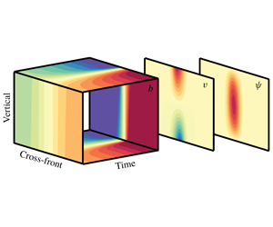
Figure 1. Frontal formation of the dimensionless zeroth-order buoyancy field (a), together with the cross-frontal planes showing the along-front velocity $v$ (b), and overturning streamfunction $\unicode[STIX]{x1D713}$ (c). The cross-frontal, vertical and time axes correspond to the dimensionless $x,z$ and $t$ axes respectively.

Figure 2. Cross-frontal profiles of the zeroth-order along-front velocity $v^{0}$ (shading) at two times defined as early frontogenesis ($t=5$, a) and late frontogenesis ($t=18$, b). Note the different colour bar axes. Superimposed in black contours is the buoyancy field, with intervals of 0.1 in non-dimensional units. Note the singularity developing during late frontogenesis. Here, $x$ and $z$ are the dimensionless cross-frontal and vertical axes, respectively, in real space.

Figure 1 illustrates the dynamical formation (in real space) of frontogenesis with the buoyancy field, and the emergence of the along-front velocity and cross-frontal overturning streamfunction. We follow Reference Shakespeare and TaylorST13 in choosing $Ro=0.4,\unicode[STIX]{x1D6FE}=0.1$ as an example for the Reference Hoskins and BrethertonHB72 case. As frontogenesis progresses, the imposed strain enhances the buoyancy gradient, which, through thermal wind balance, strengthens the along-front shear (figure 2). A useful diagnostic measure for frontal tendency is the Lagrangian evolution of the horizontal buoyancy gradient

(2.25)$$\begin{eqnarray}T_{b}^{0}=\frac{\text{D}}{\text{D}t}\frac{1}{2}\left(\frac{\unicode[STIX]{x2202}b^{0}}{\unicode[STIX]{x2202}x}\right)^{2}\end{eqnarray}$$

(Hoskins Reference Hoskins1982; McWilliams et al. Reference McWilliams, Gula, Molemaker, Renault and Shchepetkin2015), shown in figure 3. Positive frontal tendency coincides with the largest buoyancy gradient, and in late frontogenesis a negative frontal tendency adjacent to the front maximum, contributes to the sharpening the front, eventually leading to singularity. An ageostrophic overturning circulation appears in the cross-frontal plane, attempting to re-stratify the front, further contributing to frontogenesis (figure 4). The positive overturning streamfunction in figure 4 indicates a counterclockwise overturning, which is in the direction to move buoyant water over dense and stratify the frontal region. However, as the frontal region is somewhat wider than the overturning, the upper left (upper, cold-side) and lower right (lower, warm-side) buoyancy gradients are concentrated more than other regions of the front. Illustrated in figures 2(b) and 4(b), as frontogenesis progresses, the ageostrophic streamfunction strengthens and narrows, and the along-front velocity gets pinched to two points at the top, cold-side corner and bottom, warm-side corner of the frontal region of the mixed layer, and the buoyancy gradient strengthens and isopycnals come closer together and tilt – especially in these two corners, consistent with the locations of maximum frontal tendency (figure 3). The zeroth-order solution continues to strengthen and narrow, and becomes singular at these two points within a finite time. In the following section, the first-order solution effects on this process are shown.

Figure 3. Contours show buoyancy as in figure 2, shading shows the zeroth-order frontal tendency $T_{b}^{0}$.

Figure 4. Contours show buoyancy as in figure 2, shading shows the zeroth-order streamfunction $\unicode[STIX]{x1D713}^{0}$.

2.2.2 First order: turbulent fluxes

The first-order equation for the streamfunction given by (2.14) will be slightly different, depending on the type of forcing at hand

(2.26)$$\begin{eqnarray}\displaystyle & & \displaystyle \frac{\unicode[STIX]{x2202}^{2}\unicode[STIX]{x1D719}^{0}}{\unicode[STIX]{x2202}z^{2}}\frac{\unicode[STIX]{x2202}^{2}\unicode[STIX]{x1D713}^{1}}{\unicode[STIX]{x2202}x^{2}}-2\frac{\unicode[STIX]{x2202}^{2}\unicode[STIX]{x1D719}^{0}}{\unicode[STIX]{x2202}z\unicode[STIX]{x2202}x}\frac{\unicode[STIX]{x2202}^{2}\unicode[STIX]{x1D713}^{1}}{\unicode[STIX]{x2202}x\unicode[STIX]{x2202}z}+\left(\frac{\unicode[STIX]{x2202}^{2}\unicode[STIX]{x1D719}^{0}}{\unicode[STIX]{x2202}x^{2}}+\frac{1}{Ro^{2}}\right)\frac{\unicode[STIX]{x2202}^{2}\unicode[STIX]{x1D713}^{1}}{\unicode[STIX]{x2202}z^{2}}\nonumber\\ \displaystyle & & \displaystyle \quad =-\frac{\unicode[STIX]{x2202}^{2}\unicode[STIX]{x1D719}^{1}}{\unicode[STIX]{x2202}x^{2}}\frac{\unicode[STIX]{x2202}^{2}\unicode[STIX]{x1D713}^{0}}{\unicode[STIX]{x2202}z^{2}}+2\frac{\unicode[STIX]{x2202}^{2}\unicode[STIX]{x1D719}^{1}}{\unicode[STIX]{x2202}z\unicode[STIX]{x2202}x}\frac{\unicode[STIX]{x2202}^{2}\unicode[STIX]{x1D713}^{0}}{\unicode[STIX]{x2202}x\unicode[STIX]{x2202}z}-\frac{\unicode[STIX]{x2202}^{2}\unicode[STIX]{x1D719}^{1}}{\unicode[STIX]{x2202}z^{2}}\frac{\unicode[STIX]{x2202}^{2}\unicode[STIX]{x1D713}^{0}}{\unicode[STIX]{x2202}x^{2}}-\frac{2\unicode[STIX]{x1D6FE}}{Ro}\frac{\unicode[STIX]{x2202}^{2}\unicode[STIX]{x1D719}^{1}}{\unicode[STIX]{x2202}x\unicode[STIX]{x2202}z}+{\mathcal{F}}(\unicode[STIX]{x1D719}^{0}).\end{eqnarray}$$

The different turbulent flux parameterizations arise as

(2.27)$$\begin{eqnarray}{\mathcal{F}}(\unicode[STIX]{x1D719}^{0})=\left\{\begin{array}{@{}l@{}}\displaystyle \frac{\unicode[STIX]{x2202}^{4}\unicode[STIX]{x1D719}^{0}}{\unicode[STIX]{x2202}x^{3}\unicode[STIX]{x2202}z}\quad \text{(HV)},\quad \\ \displaystyle \frac{\unicode[STIX]{x2202}^{4}\unicode[STIX]{x1D719}^{0}}{\unicode[STIX]{x2202}z^{3}\unicode[STIX]{x2202}x}\quad \text{(VV)},\quad \\ \displaystyle -\frac{\unicode[STIX]{x2202}^{4}\unicode[STIX]{x1D719}^{0}}{\unicode[STIX]{x2202}x^{3}\unicode[STIX]{x2202}z}\quad \text{(HD)},\quad \\ \displaystyle -\frac{\unicode[STIX]{x2202}^{4}\unicode[STIX]{x1D719}^{0}}{\unicode[STIX]{x2202}z^{3}\unicode[STIX]{x2202}x}\quad \text{(VD)}.\quad \end{array}\right.\end{eqnarray}$$

In our theoretical framework both surface boundary conditions and interior turbulent fluxes enter at the first order and are functions of zeroth-order terms. Thus (2.26) is an inhomogeneous (with turbulent flux divergences as forcing), second-order, linear (from perturbation method), partial differential equation (PDE) which is coupled for the unknown overturning and vertical streamfunction perturbations $\unicode[STIX]{x1D713}^{1},\unicode[STIX]{x1D719}^{1}$ with non-constant coefficients, which are known functions of the zeroth-order solution. In addition to the limitations on $\unicode[STIX]{x1D700}$ and $Ro$, this analysis is also restricted to times of early frontal formation, when $\unicode[STIX]{x1D713}^{1}<O(1/\unicode[STIX]{x1D700})$ and the PDE (2.26) remains elliptic.

Note that the viscous terms are of opposite sign to the diffusive terms, but horizontal diffusivity and viscosity have the same operator, as do vertical diffusivity and viscosity. Although (2.27) suggests that diffusivity and viscosity may have opposite effects on frontal formation, an additional equation and boundary conditions that differ between viscosity and diffusivity are required in order to obtain the full uncoupled solutions for the first-order overturning and geostrophic streamfunction $\unicode[STIX]{x1D719}^{1},\unicode[STIX]{x1D713}^{1}$.

2.3 Potential vorticity

Potential vorticity, specifically Ertel PV, is a conserved quantity fundamental to geophysical fluid dynamics, and has historically been immensely useful in understanding oceanic and atmospheric dynamics (e.g. Gill Reference Gill1982; Rhines Reference Rhines1986; Pedlosky Reference Pedlosky1987; Hoskins Reference Hoskins1991; Salmon Reference Salmon1998; Kurgansky & Pisnichenko Reference Kurgansky and Pisnichenko2000). The PV is defined from the absolute vorticity ($\unicode[STIX]{x1D714}=f\boldsymbol{k}+\unicode[STIX]{x1D735}\times \boldsymbol{u}$) and buoyancy gradient

(2.28)$$\begin{eqnarray}q=(f\boldsymbol{k}+\unicode[STIX]{x1D735}\times \boldsymbol{u})\boldsymbol{\cdot }\unicode[STIX]{x1D735}b,\end{eqnarray}$$

where $\boldsymbol{u}=(\bar{U}+u,\bar{V}+v,w)$ are the background and laminar velocity fields. Note that turbulent velocities are not included in this definition of PV, which is important in the interpretation of the eddy parameterizations. Since the zeroth-order PV is assumed to be zero as in traditional frontogenesis theory, any PV in the perturbation system is associated with the first order and is a result of turbulent fluxes and boundary injection. The dimensionless first-order PV is

(2.29)$$\begin{eqnarray}\frac{q^{1}}{Ro^{2}}=\frac{\unicode[STIX]{x2202}v^{1}}{\unicode[STIX]{x2202}x}\frac{\unicode[STIX]{x2202}b^{0}}{\unicode[STIX]{x2202}z}-2\frac{\unicode[STIX]{x2202}v^{0}}{\unicode[STIX]{x2202}z}\frac{\unicode[STIX]{x2202}b^{1}}{\unicode[STIX]{x2202}x}+\left(\frac{1}{Ro^{2}}+\frac{\unicode[STIX]{x2202}v^{0}}{\unicode[STIX]{x2202}x}\right)\frac{\unicode[STIX]{x2202}b^{1}}{\unicode[STIX]{x2202}z}.\end{eqnarray}$$

Or in terms of $\unicode[STIX]{x1D719}^{1}$,

(2.30)$$\begin{eqnarray}\frac{q^{1}}{Ro^{2}}=\frac{\unicode[STIX]{x2202}b^{0}}{\unicode[STIX]{x2202}z}\frac{\unicode[STIX]{x2202}^{2}\unicode[STIX]{x1D719}^{1}}{\unicode[STIX]{x2202}x^{2}}-2\frac{\unicode[STIX]{x2202}v^{0}}{\unicode[STIX]{x2202}z}\frac{\unicode[STIX]{x2202}^{2}\unicode[STIX]{x1D719}^{1}}{\unicode[STIX]{x2202}x\unicode[STIX]{x2202}z}+\left(\frac{1}{Ro^{2}}+\frac{\unicode[STIX]{x2202}v^{0}}{\unicode[STIX]{x2202}x}\right)\frac{\unicode[STIX]{x2202}^{2}\unicode[STIX]{x1D719}^{1}}{\unicode[STIX]{x2202}z^{2}}.\end{eqnarray}$$

The PV equation (2.30), like (2.26), is also an inhomogeneous (the forcing here is the non-zero PV), second-order, linear elliptic PDE for $\unicode[STIX]{x1D719}^{1}$ with non-constant coefficients which are functions of the zeroth-order solution. As the zeroth-order solution is already known, then if given the strength of $q^{1}$, equation (2.30) can be inverted to find $\unicode[STIX]{x1D719}^{1}$. From this, $\unicode[STIX]{x1D713}^{1}$ can be found using (2.26). So, if $q^{1}$ is known, then (2.30) and (2.26) are two coupled, linear PDEs in the unknowns $\unicode[STIX]{x1D719}^{1},\unicode[STIX]{x1D713}^{1}$.

The evolution of PV (which is just $q^{1}$ as the zeroth order has zero PV) is determined by frictional and diabatic forcing through the so-called J-equation, and can be written in terms of an advective term, a frictional flux term and diabatic flux term (Haynes & McIntyre Reference Haynes and McIntyre1987; Marshall & Nurser Reference Marshall and Nurser1992; Thomas Reference Thomas2005; Benthuysen & Thomas Reference Benthuysen and Thomas2012; Wenegrat et al. Reference Wenegrat, Thomas, Gula and McWilliams2018):

(2.31)$$\begin{eqnarray}\frac{\unicode[STIX]{x2202}q}{\unicode[STIX]{x2202}t}=-\boldsymbol{u}\boldsymbol{\cdot }\unicode[STIX]{x1D735}q+(\unicode[STIX]{x1D735}\times \boldsymbol{D}_{u})\boldsymbol{\cdot }\unicode[STIX]{x1D735}b+\unicode[STIX]{x1D714}\boldsymbol{\cdot }(\unicode[STIX]{x1D735}D_{b}),\end{eqnarray}$$

where $\boldsymbol{D}_{u}$ and $D_{b}$ are the frictional and diabatic flux divergences.

Since the zeroth-order PV is uniform, the total PV equation reduces to the evolution of the first-order PV.

(2.32)$$\begin{eqnarray}\frac{\unicode[STIX]{x2202}q^{1}}{\unicode[STIX]{x2202}t}=-\boldsymbol{u}^{0}\boldsymbol{\cdot }\unicode[STIX]{x1D735}q^{1}+(\unicode[STIX]{x1D735}\times \boldsymbol{D}_{u}^{1})\boldsymbol{\cdot }\unicode[STIX]{x1D735}b^{0}+\unicode[STIX]{x1D714}^{0}\boldsymbol{\cdot }(\unicode[STIX]{x1D735}D_{b}^{1}).\end{eqnarray}$$

In the asymptotic framework, the frictional and diabatic fluxes appear only in the first order and are functions only of known zeroth-order factors,

(2.33a)$$\begin{eqnarray}\displaystyle & \displaystyle \boldsymbol{D}_{u}^{1}=\unicode[STIX]{x1D735}\boldsymbol{\cdot }F(v^{0}), & \displaystyle\end{eqnarray}$$

(2.33b)$$\begin{eqnarray}\displaystyle & \displaystyle D_{b}^{1}=\unicode[STIX]{x1D735}\boldsymbol{\cdot }F(b^{0}). & \displaystyle\end{eqnarray}$$

Likewise, the advection of the first-order PV is only carried by the known zeroth-order velocity: $(\bar{U}+u^{0},\bar{V}+v^{0},w^{0})$.

The non-dimensional form of this equation is

(2.34)$$\begin{eqnarray}\frac{\unicode[STIX]{x2202}q^{1}}{\unicode[STIX]{x2202}t}=-\left[(Ro\,u^{0}+\unicode[STIX]{x1D6FE}\bar{U})\frac{\unicode[STIX]{x2202}}{\unicode[STIX]{x2202}x}+Ro\,w^{0}\frac{\unicode[STIX]{x2202}}{\unicode[STIX]{x2202}z}\right]q^{1}+{\mathcal{D}}(v^{0},b^{0}),\end{eqnarray}$$

where the frictional and diabatic flux effects on PV have been collected into

(2.35)$$\begin{eqnarray}{\mathcal{D}}(v^{0},b^{0})=\left\{\begin{array}{@{}l@{}}\displaystyle \frac{\unicode[STIX]{x2202}b^{0}}{\unicode[STIX]{x2202}x}\frac{\unicode[STIX]{x2202}^{3}v^{0}}{\unicode[STIX]{x2202}x^{2}\unicode[STIX]{x2202}z}-\frac{\unicode[STIX]{x2202}b^{0}}{\unicode[STIX]{x2202}z}\frac{\unicode[STIX]{x2202}^{3}v^{0}}{\unicode[STIX]{x2202}x^{3}}\quad \text{(HV)},\quad \\ \displaystyle \frac{\unicode[STIX]{x2202}b^{0}}{\unicode[STIX]{x2202}x}\frac{\unicode[STIX]{x2202}^{3}v^{0}}{\unicode[STIX]{x2202}z^{3}}-\frac{\unicode[STIX]{x2202}b^{0}}{\unicode[STIX]{x2202}z}\frac{\unicode[STIX]{x2202}^{3}v^{0}}{\unicode[STIX]{x2202}z^{2}\unicode[STIX]{x2202}x}\quad \text{(VV)},\quad \\ \displaystyle \frac{\unicode[STIX]{x2202}v^{0}}{\unicode[STIX]{x2202}z}\frac{\unicode[STIX]{x2202}^{3}b^{0}}{\unicode[STIX]{x2202}x^{3}}-\frac{\unicode[STIX]{x2202}v^{0}}{\unicode[STIX]{x2202}x}\frac{\unicode[STIX]{x2202}^{3}b^{0}}{\unicode[STIX]{x2202}x^{2}\unicode[STIX]{x2202}z}\quad \text{(HD)},\quad \\ \displaystyle \frac{\unicode[STIX]{x2202}v^{0}}{\unicode[STIX]{x2202}z}\frac{\unicode[STIX]{x2202}^{3}b^{0}}{\unicode[STIX]{x2202}z^{2}\unicode[STIX]{x2202}x}-\frac{\unicode[STIX]{x2202}v^{0}}{\unicode[STIX]{x2202}x}\frac{\unicode[STIX]{x2202}^{3}b^{0}}{\unicode[STIX]{x2202}z^{3}}\quad \text{(VD)}.\quad \end{array}\right.\end{eqnarray}$$

2.4 Boundary conditions and first-order solution procedure

To evaluate first-order solutions for each of the frictional forcing cases, equation (2.34) is integrated in time using the zeroth-order terms from (2.22) and (2.23a)–(2.23c). During integration, the first-order PV is calculated, advected and accumulated.

The first-order solution is next found, for every forcing case, by solving (2.26) and (2.30) using the PV resulting from (2.34). By integrating equations (2.5a) and (2.5d), the vertical boundary conditions are solved at each time. Explicitly, the vertical boundary conditions are calculated by following the evolution of the first-order buoyancy and cross-frontal velocity at the top and bottom boundaries, for each forcing case

(2.36a)$$\begin{eqnarray}\displaystyle & \displaystyle b^{1}=\frac{\unicode[STIX]{x2202}\unicode[STIX]{x1D719}^{1}}{\unicode[STIX]{x2202}z},\quad b^{1}|_{z=0,1}=\int _{0}^{t}[-\boldsymbol{u}^{0}\boldsymbol{\cdot }\unicode[STIX]{x1D735}b^{1}-\boldsymbol{u}^{1}\boldsymbol{\cdot }\unicode[STIX]{x1D735}b^{0}+\unicode[STIX]{x1D735}\boldsymbol{\cdot }F(b^{0})]\bigg|_{z=0,1}\text{d}t, & \displaystyle\end{eqnarray}$$

(2.36b)$$\begin{eqnarray}\displaystyle & \displaystyle u^{1}=\frac{\unicode[STIX]{x2202}\unicode[STIX]{x1D713}^{1}}{\unicode[STIX]{x2202}z},\quad u^{1}|_{z=0,1}=\int _{0}^{t}[-\boldsymbol{u}^{0}\boldsymbol{\cdot }\unicode[STIX]{x1D735}u^{1}-\boldsymbol{u}^{1}\boldsymbol{\cdot }\unicode[STIX]{x1D735}u^{0}+\unicode[STIX]{x1D6FE}u^{1}+\unicode[STIX]{x1D735}\boldsymbol{\cdot }F(u^{0})]\bigg|_{z=0,1}\text{d}t, & \displaystyle\end{eqnarray}$$

(2.36c)$$\begin{eqnarray}\displaystyle & \displaystyle q^{1}|_{z=0,1}=\left.\left[Ro^{2}\frac{\unicode[STIX]{x2202}b^{0}}{\unicode[STIX]{x2202}z}\frac{\unicode[STIX]{x2202}^{2}\unicode[STIX]{x1D719}^{1}}{\unicode[STIX]{x2202}x^{2}}-2Ro^{2}\frac{\unicode[STIX]{x2202}v^{0}}{\unicode[STIX]{x2202}z}\frac{\unicode[STIX]{x2202}^{2}\unicode[STIX]{x1D719}^{1}}{\unicode[STIX]{x2202}x\unicode[STIX]{x2202}z}+\left(1+Ro^{2}\frac{\unicode[STIX]{x2202}v^{0}}{\unicode[STIX]{x2202}x}\right)\frac{\unicode[STIX]{x2202}^{2}\unicode[STIX]{x1D719}^{1}}{\unicode[STIX]{x2202}z^{2}}\right]\!\right|_{z=0,1}. & \displaystyle\end{eqnarray}$$

It is important to note that the fluxes producing PV in the preceding equations are surface turbulent fluxes associated with frontal formation. At this time we do not consider external surface forcing, such as wind stress, which has been shown to contribute additional interior PV (Thomas & Ferrari Reference Thomas and Ferrari2008).

The horizontal boundary conditions assume the laminar frontogenetic fields vanish in the horizontal, far from the front. Explicitly,

(2.37a)$$\begin{eqnarray}\displaystyle & \displaystyle v^{1}|_{x\rightarrow \pm \infty }=\frac{\unicode[STIX]{x2202}\unicode[STIX]{x1D719}^{1}}{\unicode[STIX]{x2202}x}\bigg|_{x\rightarrow \pm \infty }=0, & \displaystyle\end{eqnarray}$$

(2.37b)$$\begin{eqnarray}\displaystyle & \displaystyle u^{1}|_{x\rightarrow \pm \infty }=\frac{\unicode[STIX]{x2202}\unicode[STIX]{x1D713}^{1}}{\unicode[STIX]{x2202}z}\bigg|_{x\rightarrow \pm \infty }=0, & \displaystyle\end{eqnarray}$$

(2.37c)$$\begin{eqnarray}\displaystyle & \displaystyle q^{1}|_{x\rightarrow \pm \infty }=0. & \displaystyle\end{eqnarray}$$

The initial conditions for all first-order terms, which include the PV, $\unicode[STIX]{x1D713}^{1}$ and $\unicode[STIX]{x1D719}^{1}$ are zero, assuming turbulence and secondary circulations are negligible at $t=0$ when the front is weak. More details on the numerical methods used to illustrate the results in the following section can be found in appendix A.

Figure 5. Total frontal tendency $T_{b}=T_{b}^{0}+\unicode[STIX]{x1D700}T_{b}^{1}$ for each of the forcing cases, over a variety of $\unicode[STIX]{x1D700}$ (shades of blue), evaluated at the surface, where the zeroth-order frontal tendency maximum (black) becomes infinitely strong. For each forcing case, the maroon line represents the $\unicode[STIX]{x1D700}$ for which $T_{b}=0$. The green vertical line represents the time where the limit of the perturbation approach is reached for each forcing case: horizontal viscosity ($t=11.1$), vertical viscosity ($t=8$), horizontal diffusivity ($t=8.4$), vertical diffusivity ($t=9.1$).

4 Summary and discussion

In this study, an asymptotic approach estimates the leading-order correction of turbulent fluxes to classic theory for strain-induced frontogenesis. The system described by classic theory may capture the leading-order dynamics, but it is shown here that turbulent fluxes are likely a key secondary component missing in aligning theory with observations and model simulations, especially in the ocean where submesoscale fronts typically coexist with boundary layer turbulence, but also in lower-level atmospheric fronts. Here the effects of turbulent surface and interior fluxes of buoyancy and PV were isolated and examined.

The uncoupled first-order solutions for the along-front geostrophic velocity and ageostrophic overturning streamfunction are obtained by inverting the modified semi-geostrophic frontogenesis equation together with the first non-vanishing-order PV equation. By differentiating between horizontal and vertical eddy viscosity and diffusivity which, in reality, might be associated with parameterizations of mixed layer instabilities, boundary layer turbulence or numerical artefacts as simulated fronts approach singularity, an early understanding of the different impacts of these dissipative operators on fronts is gained. It is found that horizontal viscosity and diffusivity readily act to weaken the front, and thus are key to understanding frontal arrest, consistent with the arresting role of horizontal shear instabilities found by Sullivan & McWilliams (Reference Sullivan and McWilliams2018). Vertical viscosity and diffusivity, by contrast, act only to slow strengthening of the front at first, and later vertical diffusivity accelerates frontogenesis resembling turbulent thermal wind theory (McWilliams et al. Reference McWilliams, Gula, Molemaker, Renault and Shchepetkin2015; McWilliams Reference McWilliams2017; Crowe & Taylor Reference Crowe and Taylor2018).

As the full first-order solution depends on both turbulent boundary conditions and injected interior PV, a decomposition of the results into surface quasi-geostrophic and interior quasi-geostrophic subsystems isolates the contributions to the full solution. In most forcing cases, it is found that SQG dynamics is able to capture most of the along-front velocity and overturning streamfunction features, whereas IQG dynamics has a small contribution. The point source forcing indicates that only a small surface region near the front is needed. In the case of horizontal viscosity, the ageostrophic overturning circulation is only fully reconstructed by including both the SQG and IQG systems. Due to the nature of frontal dynamics, features tend to be localized where the front is strongest. By considering only a point source buoyancy gradient boundary condition, a good approximation to the full SQG response for both the along-front geostrophic velocity and overturning ageostrophic streamfunction was obtained. In a recent paper, Wenegrat et al. (Reference Wenegrat, Thomas, Gula and McWilliams2018) show that boundary layer turbulence can generate a source of PV at the surface, similar in magnitude to PV fluxes from wind and surface buoyancy fluxes (Thomas Reference Thomas2005). It is presently unclear whether our conclusions for the SQG and IQG systems hold true in the presence of strong surface forcing, such as downfront wind forcing, or realistic boundary layer turbulence. However, the same perturbation methods can be used while including wind forcing in (2.13), and many of the large eddy simulations being analysed include winds.

Furthermore, the asymptotic method presented in this study is derived from the semi-geostrophic equations presented in Reference Hoskins and BrethertonHB72, implying that the Rossby number is smaller than 1. However, in the submesoscale regime, both inertial and rotational forces are important and so the Rossby number is $Ro\sim 1$ (e.g. McWilliams Reference McWilliams2016). Additionally, semi-geostrophic theory has been shown to be inconsistent with $Ro\sim 1$ (Barkan et al. Reference Barkan, Molemaker, Srinivasan, McWilliams and D’Asaro2019) and curved fronts (Gent, McWilliams & Snyder Reference Gent, McWilliams and Snyder1994). The expansion parameter $\unicode[STIX]{x1D700}$ is taken to be constant; however, the realistic form is highly uncertain as it represents parameterized effects of turbulent fluxes in the submesoscale regime. The modified theory presented here merely acts as a framework to study the effects of turbulent fluxes during early frontal formation, while the semi-geostrophic assumptions and asymptotic approximation still hold.

It is intended that this framework be utilized in concert with submesoscale simulations with more realistic turbulence parameterizations or resolved turbulence to highlight important regions or aspects of such simulations. At present, large eddy simulations (Moeng Reference Moeng1984; McWilliams, Sullivan & Moeng Reference McWilliams, Sullivan and Moeng1997) are able to resolve the submesoscale dynamics and boundary layer turbulence that motivate this theory. An examination of simulations similar to those studied in Hamlington et al. (Reference Hamlington, Van Roekel, Fox-Kemper, Julien and Chini2014), Smith et al. (Reference Smith, Hamlington and Fox-Kemper2016) and Suzuki et al. (Reference Suzuki, Fox-Kemper, Hamlington and Van Roekel2016) but including strain-inducing eddies are ongoing. In all runs, a confluent region produces strong frontogenesis, but the cross-frontal scale halts at a finite width. The eventual target is finding quantitative predictions for frontal width, strength and persistence in the presence of realistic turbulent fluxes.